Modeling the effects of combining diverse software fault detection techniques

City, University of London Institutional Repository

Citation

:

Littlewood, B., Popov, P. T., Strigini, L. and Shryane, N. (2000). Modeling the effects of combining diverse software fault detection techniques. IEEE Transactions on Software Engineering, 26(12), pp. 1157-1167. doi: 10.1109/32.888629

This is the unspecified version of the paper.

This version of the publication may differ from the final published

version.

Permanent repository link:

http://openaccess.city.ac.uk/1626/

Link to published version

:

http://dx.doi.org/10.1109/32.888629

Copyright and reuse:

City Research Online aims to make research

outputs of City, University of London available to a wider audience.

Copyright and Moral Rights remain with the author(s) and/or copyright

holders. URLs from City Research Online may be freely distributed and

linked to.

City Research Online: http://openaccess.city.ac.uk/ [email protected]

techniques

Bev Littlewood

*

_{, Peter Popov, Lorenzo Strigini}

Centre for Software Reliability, City University, London

Nick Shryane

Department of Psychology, City University, London

Abstract

The software engineering literature contains many studies of the efficacy of fault finding techniques. Few of these, however, consider what happens when several different techniques are used together. We show that the effectiveness of such multi-technique approaches depends upon quite subtle interplay between their individual

efficacies and dependencebetween them. The modelling tool we use to study this

problem is closely related to earlier work on software design diversity. The earliest of these results showed that, under quite plausible assumptions, it would be unreasonable even to expect software versions that were developed ‘truly independently’ to fail independently of one another. The key idea here was a ‘difficulty function’ over the input space. Later work extended these ideas to introduce a notion of ‘forced’ diversity, in which it became possible to obtain system failure behaviour better even than could be expected if the versions failed independently. In this paper we show that many of these results for design diversity have counterparts in diverse fault detection in a single software version. We define measures of fault finding effectiveness, and of diversity, and show how these might be used to give guidance for the optimal application of different fault finding procedures to a particular program. We show that the effects upon reliability of repeated applications of a particular fault finding procedure are not statistically independent - in fact such an incorrect assumption of independence will always give results that are too optimistic. For diverse fault finding procedures, on the other hand, things are different: here it is possible for effectiveness to be even greater than it would be under an assumption of statistical independence. We show that diversity of fault finding procedures is, in a precisely defined way, ‘a good thing’, and should be applied as widely as possible. The new model and its results are illustrated using some data from an experimental investigation into diverse fault finding on a railway signalling application.

Index Terms: Software fault, fault removal, software reliability, testing,

reliability growth, diversity

*

1

Introduction

Diversity is ubiquitous in human activity. In quite mundane contexts it is common to use diversity to improve confidence: for example, I might ask a colleague to check my arithmetic in a complex calculation. The informal idea is that the mistakes he might make will differ from those that I might make, and our arriving at the same answer suggests that neither of us has made a mistake, thus increasing my confidence that the answer is correct.

The key to the approach is, of course, the presence of intellectual differences in the two procedures. Note that this notion of diversity differs fundamentally from that of

redundancy in which there is simply replication (e.g. of a component to increase

hardware reliability) of exactly similar items: I would have less trust in my own exact replication of the calculation than in the different calculation of my colleague.

In software, design diversity has been proposed as a means of achieving higher reliability than could be achieved (for the same outlay of effort) from a single version. Such design diverse software architectures have seen fairly widespread industrial use [Rouquet and Traverse 1986]. In the early days, it seems that the motivation for the approach owed a great deal to the hardware redundancy metaphor, to the extent that independence of failures of the versions was seen as the goal (albeit recognised as difficult to achieve). Later, several experiments [Eckhardt, Caglayan et al. 1991; Knight and Leveson 1986] showed that such a goal was probably unrealistic: version failures tended to be highly dependent. Thus, whilst considerable improvement in reliability could be expected from a multi-version architecture compared with the reliabilities of the single versions, this nevertheless fell far short of what would have been achieved if these versions failed independently.

An insight into the nature of the dependence came from a probabilistic model developed by Eckhardt and Lee (EL) [Eckhardt and Lee 1985], and later generalised by Littlewood and Miller (LM) [Littlewood and Miller 1989]. The basic idea here is that different inputs have different ‘difficulty’ - roughly, the difficulty (and thus proneness to failure) faced by the designer of the software in providing a correct way of processing them. As an example, consider an aircraft flight control system: we might think of the set of inputs corresponding to landing in turbulent wind-shear as ‘more difficult’ than those corresponding to straight and level flight in calm conditions. It is shown in EL that this variation of difficulty induces dependence upon the version failures, even though these might fail conditionally independently. The intuition here is simple. If there are two versions, A and B, and for a particular input we see that A has failed, we infer that the input was ‘probably difficult’, and that B is therefore more

likely to fail. This is true even though, for every input, the versions fail (conditionally)

independently - and it is this conditional independence that is the difficult goal to which the systems designers aspire.1

1

In more precise mathematical terms, we say that A and B fail conditionally independently if, for every possible input, x,

P(A and B both fail| x)=P(A fails| x ). P(B fails| x)

They fail unconditionally independently, on the other hand, if for a randomly chosen (i.e. unknown) input

P(A and B both fail) =P( A fails). P(B fails) .

The LM model generalises EL by introducing the possibility that the procedures used by the A and B teams may be different (‘forced diversity’), and thus that what the

A team finds difficult may be different from what the B team finds difficult. It

introduces the possibility that diversity can be forced so that the versions will fail in

negatively correlated ways - thus giving better system reliability even than from

independence. It has to be admitted, however, that such an outcome may be unlikely in practice.

A major conclusion to be drawn from these models is that there are traps for the unwary in simple reliability models of multi-version software. In particular, assumptions of conditional independence generally do not carry through to justify claims of unconditional independence.

Although the models are quite subtle, their intuitive underpinnings are quite simple. What is surprising is their very wide applicability. In this paper we shall show that similar results apply to diversity in the fault detection processes that are applied to a

single software version. Once again, the benefits that we get from the application of

diverse fault detection procedures may sometimes be less than we could expect under naïve assumptions of independence. However, the possibility of obtaining real benefits from forced diversity, and predicting the extent of these benefits, seems more plausible here than it does in the case of design diversity.

2

A model of diverse fault detection

Consider a single program that is going to be subjected to two different (‘diverse’) fault detection procedures, A and B. For simplicity we shall assume that the program is demand-based (e.g. a nuclear reactor protection system). As an example, one of the fault detection procedures might be testing, in which the program is subjected to a particular number of demands; another might be some form of static analysis, for which a certain amount of staff effort is allocated.

The practical intuition here is that each fault detection procedure varies in its efficacy from one fault to another, and that the different procedures may target different faults most effectively. That is, procedure A may be stronger on those faults for which

B is weaker. This is a kind of forced diversity - applied to fault detection - similar to the

forced diversity of design and development methods in the LM model. The difference here is that the diverse fault detection is being applied to a single program. We shall try to keep the notation here as close as possible to that of LM, so that readers familiar with this model can see the similarities.

We shall assume that there is at most one fault associated with each input. One way of thinking of a fault in a program is as the set of all inputs that change from being ‘faulty’ (i.e. cause a failure when executed) to ‘non-faulty’ (i.e. do not cause a failure when executed) when the program is changed ‘in order to remove a fault’ [Frankl, Hamlet et al. 1997].

It is now possible to imagine all possible faults that might be in a program. We shall label these with the natural numbers: {i: i=1,2,3,...}. Clearly, some of these faults will be more likely to be present in a particular program than others. Let

set of all programs. Thus the single program that we are dealing with can be regarded as having been randomly selected from this set of possible programs.

Of particular interest is the probability distribution {pi*} where

pi*=

pi

p_i

i

∑

= P(randomly selected fault is fault i) (2)

For any particular fault, i , we define A(i) to be the probability that a (randomly

chosen) application of the fault detection procedure A fails to find this fault. The key idea, as in EL, is that this function varies from one fault to another. For a particular fault it can be thought of as the ‘difficulty’ of finding that fault using procedure A, similar to the ‘difficulty’ of inputs in the EL and LM models.

If, as an example, we think of A as being the execution of n operational test cases - i.e. chosen at random using the operational profile over the input space - then clearly each such ‘test’ will either reveal the fault i or it will not. If we were to repeat this procedure many times, generating many sequences, each of n inputs, from the operational profile, A(i) can be thought of as the proportion in which the procedure

fails to detect the fault i.

The difficulty functions determine the efficacy of the fault detection procedures. For example, we can define a measure of A’s fault-detection efficacy as the chance that an ‘average’ or ‘typical’ fault is found in a (randomly chosen) application of A. In order to keep our notation in step with that of the EL and LM models we shall generally express the results here in terms of ineffectiveness (cf. unreliability in the earlier models) of the fault detection procedure A:

P(A fails to detect a randomly chosen fault )

= pi*. A(i)=Ep*

(

A(i)

)

i

∑

(3)

where the notation Ep* indicates a mean obtained with respect to the probability

distribution p*. We have the following:

Result 1:

E(number of faults in program undetected after the application of A)

= E_p*

(

_A(i)

)

.E(number of faults in program before the application of A) (4)

and

E(number of faults detected by application of A)

Proof:

E(number of faults undetected in program after the application of A)

= P(fault i present and is not detected by application of A)

i

∑

= p_i

i

∑

. _A(i)= p_i

i

∑

   

 pi*. A(i) i

∑

 

 



= Ep*

(

A(i)

)

.E(number of faults in program before the application of A)

The second part of the result follows trivially.

QED

We shall define the effectiveness of A to be

1−ineffectiveness = 1

(

−E_p*

(

_A(i)

)

)

which is simply the probability that A successfully detects a randomly chosen fault.

For a different fault removal procedure, B, we could define similarly B(i) and

Ep*

(

B(i)

)

. If Ep*

(

A(i)

)

were greater than Ep*

(

B(i)

)

we would say that A is less

effective at finding faults than B, in the sense that it would be expected to detect fewer faults.

We shall now show that, corresponding to the EL result in design diversity, we have here a lack of independence in the effects of successive applications of the same fault detection procedure, and that this implies a law of diminishing returns. Consider again, as an example, the situation where A is operational testing. An interesting question is how the effectiveness of this kind of testing changes as we apply more randomly chosen operational inputs. Consider the case where we carry out two such fault detection procedures, independently, A₁ and A₂. Each comprises n independently randomly chosen inputs, and the two sequences of n inputs are independent of one another. In general in such a case of a double application of a procedure we have:

Result 2:

P(A1 and A2 fail to detect a randomly chosen fault )

≥P(A₁ fails to detect a randomly chosen fault ).

P(A₂ fails to detect a randomly chosen fault )

(6)

or, equivalently,

P(A₂ fails to detect a randomly chosen fault | A₁ failed)

≥P(A₂ fails to detect a randomly chosen fault ) (7)

Proof:

Clearly, for each fault i

i.e. failures of the two applications of the fault detection procedure are conditionally

independent, for every fault.

For a randomly selected fault, on the other hand

P(A₁ and A₂ fail to detect a randomly chosen fault ) = pi*. A

2

(i)= Ep* A

2 (i)

(

)

i

∑

≥[Ep*

(

A(i)

)

]

2 (8)

since Ep* A

2 (i)

(

)

−[Ep*

(

A(i)

)

]

2 ₌

Var

(

A(i)

)

≥0

QED

It is easy to show (cf. the EL and LM models) that there is equality in these expressions if and only if A(i)= identically for all faults. Clearly, it seems certain

that no real fault finding procedures have the property of completely constant difficulty with respect to all faults.

Another way to think of these expressions is in terms of the number of faults you would expect to detect in a program by applying a particular fault finding procedure. Clearly, if you apply the procedure twice you would not expect to find twice as many faults as applying it just once - informally, there is a chance that some of the faults that could have been found in the second application would already have been found in the first application. This would be true even if there were complete independence in the two applications (i.e., in the terminology of the model, A(i)=

identically for all faults). What the result above says is that things are even worse than this independence case when there is variation of difficulty: i.e. you would expect to find even fewer faults with two applications than you would if you could assume independence.

These results depend on the fact that, even though the two applications of the fault detection procedure are conditionally independent for all faults, they are not unconditionally independent. Informally, the failure of the first application of A to find the fault suggests that it is a ‘difficult’ fault for A, and thus that a second application of

A will also be likely to fail to find it. If the first application of operational testing has

revealed only a few faults, for example, we should tend to lose confidence in the likely effectiveness of a second application of the procedure.

This result corresponds to our intuition. Most people would not persevere with putting all their fault detection effort into a single procedure, such as, for example, inspection or operational testing. Rather they would tend to expect there to be a law of diminishing returns operating, whereby most of the faults that can easily be detected by a procedure, are eventually detected. At some point, therefore, it would seem sensible to cease one fault detection activity and switch to another, which it is hoped will target a different class of faults. We now examine this case of diverse fault removal: the reader familiar with the earlier models of design diversity will see that the following is similar to the LM model, as the former was similar to EL.

Consider now, therefore, two different fault detection procedures A and B:

Result 3:

P(A and B fail to detect randomly selected fault )

and

P(B fails to detect a randomly chosen fault | A failed)

>P(B fails to detect a randomly chosen fault ) (10)

if and only if

Covp*

(

A(i), B(i)

)

>0 (11)

Proof:

We assume conditional independence in the following obvious way:

P(A and B fail to detect fault i | i present)= A(i). B(i) (12)

for every fault i.

For a randomly selected fault, on the other hand:

P(A and B fail to detect randomly selected fault )

= pi* i

∑

. A(i). B(i)=Ep*

(

A(i). B(i)

)

(13)

which, in general

>E_p*

(

_A(i)

)

. E_p*

(

_B(i)

)

=P(A fails to remove randomly selected fault ).

P(B fails to remove randomly selected fault )

if and only if Cov_p*

(

_A(i), _B(i)

)

>0

QED

In other words, you would expect to find fewer faults by applying A and B when Cov_p*

(

_A(i), _B(i)

)

>0 than you would if you could assume independence (and, of course, this latter expected number will be smaller2 than the sum of the numbers you would expect from a single application of A and a single application of B).

There is an intriguing possibility of better than independent behaviour of the two procedures if the covariance is negative. Such negative covariance would be possible whenever the different fault detection procedures targeted different types of faults, i.e. whenever the ‘difficult’ faults for one procedure are the ‘easy’ ones for the other, and vice versa.

An expectation of something like negative covariance does seem to lie behind the intuition of those people involved in software verification and validation, for whom an eclectic mix of different fault finding procedures is preferred to the extensive application of a single one. What is novel in the work reported here is that we introduce

2

the possibility of measures that characterise this desirable diversity between different procedures. Interestingly, the measures seem more amenable to statistical estimation than the corresponding ones in design diversity, as we shall see in a preliminary example in Section 6.

3

Effects on reliability

The results of the previous section concern the efficacy of different procedures at finding faults. Of course, knowing that a procedure is good at finding faults is not the same as knowing that it is good at improving reliability (when the faults that are detected are removed). It is well-known that in real programs different faults can have very different impacts on a program’s unreliability [Adams 1984]: a fault-finding procedure that was very efficient at finding ‘small’ faults could be very inefficient at finding ‘large’ ones, and thus at improving reliability. A ‘good’ fault finding (and removal) procedure is one that tends to improve reliability most efficiently [Frankl, Hamlet et al. 1997]. We now show that similar results to those above also apply to the efficacy of fault finding procedures in improving reliability. Throughout this section we shall assume that when a fault is detected it is removed with certainty.

Let

i =P(fault i is activated by randomly selected

input and is detected and fixed ) (14)

The unreliability of the program is then

P(program fails on randomly selected input )= _i

i

∑

(15)

and

i*= i

i i

∑

= P(randomly selected failure caused by fault i)

(16)

Consider now the effect of applying the fault removal procedure A on the program unreliability, i.e. on the probability that it fails on a randomly selected input.

Result 4:

P(program fails on randomly selected input following application of A)

= E*

(

A(i)

)

.P(program fails on randomly selected input before applying A)

Proof:

P(program fails on randomly selected input following application of A)

= P(fault i activated following application of A)

i

∑

= P(A has not removed fault i and it is activated )

i

∑

= i. A(i)= i i

∑

   

 i* i

∑

. _A(i)

 

 



i

∑

= E*

(

A(i)

)

.P(program fails on randomly selected input before applying A)

QED

Thus the factor E _*

(

_A(i)

)

can be seen as a measure of the ineffectiveness of procedure A in improving reliability: the smaller this is, the better. Similarly, its complement can be thought of as the effectiveness.

Consider now the application of fault removal procedure A twice, A₁, A₂. We have a result similar to Result 2:

Result 5:

The ineffectiveness of A₁ and A₂ together is greater than or equal to the product of the ineffectiveness of A₁ and the ineffectiveness of A_2.

Proof:

P(program fails on randomly selected input following application of A1 and A2)

= P(fault i activated following application of A₁ and A₂)

i

∑

= P(A₁ and A₂ have not removed fault i and it is activated )

i

∑

= i. A

2

(i))= _i

i

∑

i

∑

i*

i

∑

. _A2 (i)

= E_{* A}2 (i)

(

)

. P(program fails on randomly selected input before applying A₁ and A₂)

≥ E _{* A}2 (i)

(

)

(

)

2

P(program fails on randomly selected input before applying A₁ and A₂)

QED

As before, there will be equality here if and only if _A(i)≡ for some constant , identically for all faults.

would expect under independence, since E * A

2 (i)

(

)

is always less than E

(

*

(

A(i)

)

)

2 . This is, again, the analogue of the EL result.

If, on the other hand, we apply diverse fault removal procedures, A and B, we find, as before, that we can do better than this:

Result 6:

The ineffectiveness of applying A and B together is greater than the product of the ineffectiveness of A and the ineffectiveness of B if and only if Cov *

(

A(i), B(i)

)

>0 .

Proof:

P(program fails on randomly selected input following application of A and B)

= P(fault i activated following application of A and B)

i

∑

= P(A and B have not removed fault i and it is activated )

i

∑

= i. A(i). B(i)= i i

∑

   



i

∑

i*

i

∑

. A(i). B(i)

 

 



= E*

(

A(i). B(i)

)

.P(program fails on randomly selected input before applying A and B)

>E *

(

A(i)

)

.E *

(

B(i)

)

. P(program fails on randomly selected input before applying A and B)

if and only if Cov _*

(

_A(i), _B(i)

)

=E _*

(

_A(i). _B(i)

)

−E _*

(

_A(i)

)

. E _*

(

_B(i)

)

>0

QED

Thus the factor E _*

(

_A(i). _B(i)

)

, which determines the reduction in unreliability (improvement in reliability) coming from the successive applications of A and B, can be either smaller or larger than the equivalent expression that assumes independence, E *

(

A(i)

)

. E *

(

B(i)

)

, according to whether the covariance

Cov _*

(

_A(i), _B(i)

)

is positive or negative. We would like it to be smaller, i.e. the covariance to be negative.

4

Optimal allocation of fault detection procedures

The results of the previous two sections show that, in a limited sense, negative correlation between the difficulty functions of two fault finding procedures is ‘a good thing’. In practice, of course, this does not tell us how to deploy A and B when we have a fixed amount of effort available. There will be a trade-off between the efficacies of the individual fault finding procedures and their dependence, and it may be that it will be most effective to use only A (or only B). In this section we provide some tentative advice for optimal allocation of procedures, by showing that, when we believe

Consider the case where we have two fault finding procedures, A and B. For example, let A, as before, be operational testing; let B be a form of static analysis. Assume that we are indifferent between a randomly chosen application of A (i.e. a randomly chosen set of operational inputs), and a randomly chosen application of B (i.e. a particular application of the static analysis procedure). That is, if we were to apply only one of these procedures to our program we would have no preference between them. Then we can show that it is always better to apply A once and B once rather than either of them twice; more precisely:

Result 7:

If E * A

2 (i)

(

)

=E * B

2 (i)

(

)

then

P(program fails on randomly selected input following application of A and B)

<P(program fails on randomly selected input following application of A1 and A2) and

P(program fails on randomly selected input following application of A and B)

<P(program fails on randomly selected input following application of B1 and B2)

Proof:

By the Cauchy-Schwarz inequality

E *

(

A(i). B(i)

)

< E * A

2 (i)

(

)

(

)

1

2

E * B

2 (i)

(

)

(

)

1

2

=E * A

2 (i)

(

)

=E * B

2 (i)

(

)

so

P(program fails on randomly selected input following application of A and B)

= E*

(

A(i). B(i)

)

P(program fails on randomly selected input before fault finding )

<E * A

2 (i)

(

)

P(program fails on randomly selected input before fault finding )

= P(program fails on randomly selected input following application of A1 and A2) and similarly for B₁ and B₂.

QED

A similar result holds for efficacy defined in terms of the expected numbers of faults removed: we would expect more faults to be removed by an application of A and

B than by two applications of A or two of B (subject to a similar indifference

assumption3

). The similarity of this result to that just proved is just a generalisation of the parallelism that we have seen between the results involving efficacy of fault removal (results 1-3) and those involving improvement in reliability (results 4-6). The proof

3

follows simply and will not be given here: similar comments apply to all the results of this section.

This result can be generalised to more than two fault finding procedures. Thus for three procedures A, B and C, we have a choice between the following applications (in an obvious notation): AAA, BBB, CCC, AAB, AAC, ABB, . . . , BCC, ABC. If

we are indifferent between all the single fault finding procedures

E * A

3 (i)

(

)

=E * B

3 (i)

(

)

=E * C

3 (i)

(

)

(18)

and between all those using two procedures

E * A

2

(i). B(i)

(

)

=E * A

2

(i). C(i)

(

)

=E * A(i). B

2 (i)

(

)

. . . (19)

it can be shown that E *

(

A(i). B(i). C(i)

)

is smaller than all these other inefficiency

factors, and so the greatest improvement in reliability will come by applying ABC.

More generally, when k different fault finding procedures are available, subject to certain indifference assumptions between them, it is best to use all of them and to spread their use as evenly as possible. Thus, for example, if we are prepared to apply 5 randomly chosen fault finding procedures, but only have 3 different types, then

AABCC is better than AAABC, etc. This can be expressed in general as:

Result 8:

Let (n1,n2,...nk) represent the allocation of ni randomly chosen applications of fault

finding procedure i (i=1,2,...k),

ni =n i=1

k

∑

.

Assuming indifference between allocations that merely involve permutations of procedures, the best allocations (there will generally be more than one) are those for which

n k

[ ]

≤n_i ≤

[ ]

n_k +1, 1≤i≤k (20)

where [x] denotes the greatest integer not greater than x.

Proof:

See [Littlewood and Miller 1989]

If A were, as before, operational testing, and B were a type of static analysis, we would need to select a number of test cases for the ‘unit’ of operational testing, and an ‘amount’ of static analysis (e.g. the time for an analyst of a particular competence) so that we would be indifferent between (randomly chosen) single applications of each of the two4

. It seems likely that in practice there is usually some appropriate ‘cost’ variable that will allow us to define units of different fault finding procedures that we think are equivalent in their likely impact upon reliability. This result can be seen as a formalisation of the kind of informal allocation between different procedures that is carried out on a day-to-day basis during real system verification and validation.

5

Degrees of diversity

It seems intuitively plausible that, if diversity is ‘a good thing’, then more diversity is better than less. In this section we present a measure of diversity between pairs of fault finding procedures that gives meaning to the notion of ‘more diverse’.

Consider the two procedures A and B. Since a procedure is completely characterised by its difficulty function over faults, , we can define a distance between the two procedures in this function space:

A− B

2

=E *

(

A(i)− B(i)

)

2

(

)

(21)

Clearly, _A− _B 2 >0 unless _A(i)≡ _B(i) . It follows trivially that

E *

(

A(i). B(i)

)

<E * A

2 (i)

(

)

=E * B

2 (i)

(

)

if we assume indifference between the procedures when applied singly. This is precisely Result 7, which says that the improvement in reliability by applying A and B is better than that obtained by applying either twice.

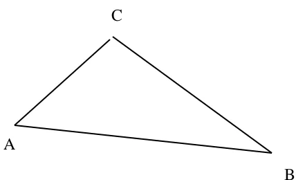
Consider now the case where three procedures are available, A, B and C, but it is only feasible (e.g. on cost grounds) to apply two of them. Suppose further that we believe that A and B are more diverse, in the sense of (21), than are A and C, or B and

C. This is shown schematically in Figure 1:

4

A

[image:15.595.199.413.131.261.2]

B C

Figure 1

Result 9:

If A and B are more diverse than B and C, i.e.

A− B > B − C ,

and we are indifferent between two-fold applications of each of the three procedures, i.e.

E * A

2 (i)

(

)

=E * B

2 (i)

(

)

=E * C

2 (i)

(

)

, then

E *

(

A(i). B(i)

)

<E *

(

B(i). C(i)

)

[The proof is trivial]

In other words, if we have a choice of two procedures that are more diverse than another pair, we should prefer the former, all things being equal.

6

Example

Data to illustrate parts of the new model were obtained from a study into the verification of safety-critical computer programs used in railway signalling systems: this experiment pre-dated the development of the model described here.

Observational fieldwork conducted on-site at a number of railway signalling contractors had revealed qualitative differences between faults typically found by diverse verification methods, in this case static code checking and functional testing. However, variability in the complexity of work and personnel expertise found at different contractors’ sites, and most importantly the lack of independence between the fault-finding methods as practised in situ, could have been confounding this result.

period of ‘core’ instruction in railway signalling principles common to all participants, half were then given specific training for the code checking task and half were trained for the testing task.

Participants were then required to verify two simulated railway signalling programs, either by code checking or functional testing as appropriate. Each program was seeded with eight faults (taken from those found during the fieldwork), each of the faults being potentially detectable with either verification method. The dependent variable was thus the proportion of the total faults detected by each participant, the independent variable being whether the participant was a checker or a tester. For reasons that are beyond the scope of the present paper, some participants were excluded from the experiment, leaving a total of twenty-seven checkers and thirty-six testers (Further information on this issue, and on the experimental task in general, can be found in [Westerman, Shryane et al. 1997; Westerman, Shryane et al. 1995]; for more information on the railway signalling task on which it is based, see [Shryane, Westerman et al. 1998]).

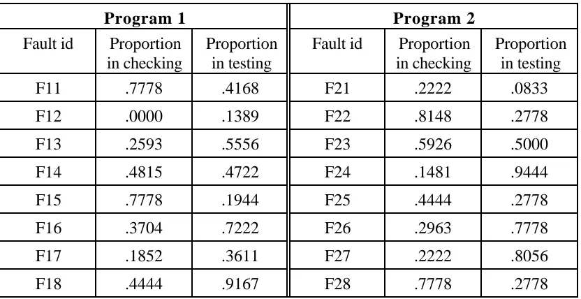
The raw data are shown in Table 1. Here the entries in the table are, for each fault, the proportion of the individuals in that part of the experiment who were unsuccessful in finding the fault: for fault i and procedure A we take this to be an estimate of A(i) in the notation of the model. If we treat each program separately, we

have p_i*=1/8 for each of the eight faults in each program. If we let A represent checking and B represent testing, it is then easy to show that for Program 1 (estimates of) the relevant parameters of the model are:

Program 1 Program 2

Fault id Proportion Proportion Fault id Proportion Proportion in checking in testing in checking in testing

F11 .7778 .4168 F21 .2222 .0833

F12 .0000 .1389 F22 .8148 .2778

F13 .2593 .5556 F23 .5926 .5000

F14 .4815 .4722 F24 .1481 .9444

F15 .7778 .1944 F25 .4444 .2778

F16 .3704 .7222 F26 .2963 .7778

F17 .1852 .3611 F27 .2222 .8056

[image:16.595.86.502.429.643.2]

F18 .4444 .9167 F28 .7778 .2778

E_p*

(

_A(i)

)

=0.412, E_p*

(

_B(i)

)

=0.472

Ep* A

2 (i)

(

)

=0.235, Ep* B

2 (i)

(

)

=0.282

Ep*

(

A(i). B(i)

)

=0.199, Ep*

(

A(i)

)

Ep*

(

B(i)

)

=0.194

Covp*

(

A(i), B(i)

)

=0.0040

(22)

and for Program 2:

E_p*

(

_A(i)

)

=0.440, E_p*

(

_B(i)

)

=0.493

Ep* A

2 (i)

(

)

=0.253, Ep* B

2 (i)

(

)

=0.329

Ep*

(

A(i). B(i)

)

=0.179, Ep*

(

A(i)

)

Ep*

(

B(i)

)

=0.217

Covp*

(

A(i), B(i)

)

=−0.0381

(23)

Notice that the efficacies of A and B are roughly similar between the two programs, but that B seems to be consistently worse than A. Also, there seems to be ‘more diversity’ between A and B in their application to Program 2 than to Program 1: there is negative correlation between the difficulty functions in the case of Program 2, but small positive correlation for Program 1.

After two applications of A to Program 2, we would expect 25.3%5

of faults to be undetected; after two applications of B, 32.9% of faults to be undetected; but after an application of each of A and B, we would expect only 17.9% of faults to be undetected. Thus, in this case we would expect the application of A and B to be more effective than a double application of A or of B. This is so even though we are not indifferent between A and B here: in fact A seems significantly better than B (and AA than BB). Here the naïve ‘independence’ argument would seriously underestimate the efficacy of

AB, suggesting that it would leave 21.7% of faults undetected, rather than the correct

figure of 17.9%.

For Program 1, the corresponding figures are: after two applications of A, we expect 23.5% of the faults to be undetected; after two applications of B, 28.2%; and after one application of A and one of B, 19.9%. Once again, the diverse application of

AB is better than either AA or BB, even though the difficulty functions show slight

positive correlation - but this superiority is less dramatic than in Program 2, where the procedures have negatively correlated difficulty functions. In this case the naïve ‘independence’ assumption would slightly overestimate the efficacy of AB, suggesting it would leave 19.4% of faults undetected rather than the correct figure of 19.9%.

The differences in the examples above, (22) and (23), suggest how we might use this model in practice. If we believe that the effectiveness of successive applications of particular diverse fault finding procedures will vary from one class of problem to another (e.g. real-time versus non-real-time), but are constant within each problem class, then we should strive to estimate the parameters of the model for each problem class. Thus if we had two sets of data, like those for Programs 1 and 2, corresponding

5

to two different types of program, we could estimate the parameters relating to their different behaviours.

If, on the other hand, we have no reason to believe that there are such differences, we should regard data from all programs as being evidence to be used for obtaining a single set of parameter estimates for the model. If we aggregate the above data in this way, treating each program as having been sampled with constant probability from a population of programs, we find that the model parameters are estimated as follows:

E_p*

(

_A(i)

)

=0.426, E_p*

(

_B(i)

)

=0.483

Ep* A

2 (i)

(

)

=0.244, Ep* B

2 (i)

(

)

=0.306

Ep*

(

A(i). B(i)

)

=0.189, Ep*

(

A(i)

)

Ep*

(

B(i)

)

=0.206

Covp*

(

A(i), B(i)

)

=−0.0168

(24)

Now, after a double application of A we would expect 24.4% of faults to be undetected; after a double application of B, 30.6%; and after application of a single A and a single B, 18.9%. Once again, rather informally, the strong diversity of the procedures, indicated by their negative correlation, means that an application of each of

A and B is best, even though A is clearly superior to B (and AA to BB). Once again,

because of the negative correlation of the difficulty functions, the naïve independence estimate gives an underestimate of the efficacy of AB: it suggests that this will leave behind 20.6% of faults undetected whereas the true figure is 18.9%.

These results illustrate the quite subtle interplay that there can be between the efficacies of the individual procedures and their ‘degree of diverseness’: in general we need to know all first and second moments of the (random variable) difficulty functions before we can determine the most effective mix of procedures. We have been able to show earlier that by imposing certain indifference constraints it is possible to know that

AB will be better than AA or BB whenever there is negative correlation. When we

cannot make such assumptions, however, mere diverseness, as represented by negative correlation between the difficulty functions, is not sufficient to ensure that it will be best to apply both procedures. It is easy to show that when there is negative correlation AB will always be better than the worst of AA and BB, but it could be either better or worse than the better of these. Equally, negative correlation is not necessary for AB to be superior to AA and BB: there can be benefit in diversity even when the procedures are positively correlated, as in the case of Program 1.

These comments notwithstanding, the results of Section 3 (and similarly those of Section 4) do seem like a promising way of giving designers advice about the best fault finding approach when, as is sometimes the case, we are in a position to balance the efficacies of different procedures by applying one of them ‘more’ or ‘less’ extensively. Thus, in the example here we might require the testers to spend more time - examining more test cases - so as to make Ep*

(

B(i)

)

=Ep*

(

A(i)

)

in (24). Whenever

we can do this, we shall have a guarantee that AB will be superior to AA or BB, even when we do not have the detailed extra information about the parameters of the model that we have from this controlled experiment.

of faults, rather than with the faults themselves, and it can be illustrated again by the railway data example.

The psychologists who devised this experiment were interested in investigating differences in diverse fault finding between different types of fault; details can be found in the papers cited earlier, but the following is a brief account. As part of the signalling system design task, engineers must translate information contained in track layout plans, regarding permitted directions of movement of trains over track sections, into a machine-readable label. Configurations of track sections are variable, and so a rule is used to specify the mapping between the label and the route of the train. Engineers made mistakes when generating the labels, and more importantly when performing an independent check of others’ work, a vital part of the rigorous verification and validation process to which safety critical systems must be subjected. Faults in Programs 1 and 2 varied as to whether the code involved the use of such train subroutes (S) or not (N). There were thus two classes of fault, S and N: in Table 1, faults F11, F15, F22, F25 were of type S and the remaining 12 faults were of type N.

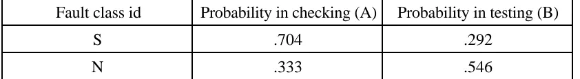
We can now easily compute a table similar to Table 1, but involving classes of

faults rather than the individual faults themselves:

Fault class id Probability in checking (A) Probability in testing (B)

S .704 .292

[image:19.595.84.505.348.406.2]

N .333 .546

Table 2 Estimates of the probabilities that a randomly chosen fault of type S (N) will fail to be detected by an application of procedure A (B), obtained from the data of Table 1 aggregated over the two programs.

In an obvious notation, the entries of Table 2 can be thought of as estimates of

A(s) , etc. We can now perform calculations similar to those carried out earlier, using

pS*=0.25, pN*=0.75 , to obtain:

Ep*_classes

(

A(i)

)

=0.426, Ep*_classes

(

B(i)

)

=0.483

E_p* classes A

2 (i)

(

)

=0.207, E_p*

classes B

2 (i)

(

)

=0.245

Ep*classes

(

A(i). B(i)

)

=0.188, Ep*classes

(

A(i)

)

Ep*classes

(

B(i)

)

=0.206 Covp*_classes

(

A(i), B(i)

)

=−0.0178

(25)

actual difficulty functions from Table 1). Thus, for example (in an obvious notation),

the ineffectiveness of AA based on the full fault data can be expressed as:

Ep* A

2 (i)

(

)

= pS*.Ei∈S A

2 (i)

(

)

+pN*.Ei∈N A

2 (i)

(

)

= p_S*. E

(

(

_i∈S

(

_A(i)

)

)

2+Var_i∈S

(

_A(i)

)

)

+p_N*. E

(

(

_i∈N

(

_A(i)

)

)

2 +Var_i∈N

(

_A(i)

)

)

= Ebetween classes

(

Ewithin classes

(

A(i)

)

)

2

+Ebetween classes

(

Varwithin classes

(

A(i)

)

)

(26)

and similarly for B.

That is, the first term - which we have called Ep*classes A

2 (i)

(

)

in the condensed notation of (25), and which takes the value 0.207 - underestimates the true value by an amount E_{between classes}

(

Var_{within classes}

(

_A(i)

)

)

=0.037. This agrees with (24), since 0.244 = 0.207+0.037.

What is interesting and surprising, though, is the closeness between the ineffectiveness estimates of AB in (24) and (25). We would expect these to differ since the expression in (24) can be expressed:

E_p*

(

_A(i). _B(i)

)

= p_S*.E_i∈S

(

_A(i). _B(i)

)

+ p_N*.E_i∈N

(

_A(i). _B(i)

)

= p_S*. E

(

_i∈S

(

_A(i)

)

E_i∈S

(

_B(i)

)

+Cov_i∈S

(

_A(i), _B(i)

)

)

+pN*. E

(

i∈N

(

A(i)

)

Ei∈N

(

B(i)

)

+Covi∈N

(

A(i), B(i)

)

)

= E_{between classes}

(

E_{within classes}

(

_A(i)

)

.E_{within classes}

(

_B(i)

)

)

+Ebetween classes

(

Covwithin classes

(

A(i), B(i)

)

)

(27)

The first term here is the approximation using aggregated fault class data from (25), which in the condensed notation used there is E_p*classes

(

_A(i). _B(i)

)

=0.188. The second term is the weighted average, using p_S*=0.25 and p_N*=0.75 respectively, of the covariances of the A and B difficulty functions for the different fault classes, which take the values 0.000 and 0.001 respectively (to 3 decimal places). The smallness of these is the reason for the closeness of the estimate of AB effectiveness based on the aggregated fault class data to the correct figure based on the full fault data.

The surprise here is that the devisors of the experiment have managed to arrive at fault classes, S and N, for each of which the difficulty functions of A and B are almost independent. It would be worth investigating whether this can be done in other circumstances: if it can, we shall be able to obtain accurate estimates of AB ineffectiveness even from aggregated fault class data.

The practical advantage of the treatment via classes of faults, rather than the individual faults themselves, is as follows. Individual faults are likely to be ‘sparse’. If we collect our data from only a few real programs, we are likely to see each fault in no more than one program, in contrast to the artificially seeded programs which are used repeatedly in the experiment. There will thus be no opportunity to estimate the probabilities pi*. If, on the other hand, we can identify meaningful and interesting

be able to predict the efficacy of diverse fault finding, as in (25), for an entirely novel

program if we can estimate the p *classes values for this new program.

An especially desirable situation would be achieved if the fault classes identified had the special property that was fortuitously obtained in this experiment, i.e., that the difficulty functions for different fault detection methods have zero covariance over the different fault classes. Then, estimating the mean of the functions for each {fault class, fault detection method} combination - which is much simpler than estimating complete distributions - would be sufficient to allow useful predictions in many cases. As can be seen from (26), the predictions would be exact for combinations of diverse methods, and optimistic for repeated applications of one method: when the methods are ‘diverse’ enough, these estimates would provide sufficient conditions for a project manager to decide in favour of combining two diverse methods.

Essentially this approach reuses the hard-won data such as that of Table 2, gained from past experience of other projects or from experiments, by applying it to prediction in a new context. Whilst this does require that we know, or are prepared to estimate, the new p *classes values, this is a feasible task in contrast to attempting to do

so for the set of all faults. As an example, if we believe that for the new program

p_S*=0.50, p_N*=0.50 , we obtain:

E_p*

classes

(

A(i)

)

=0.519, Ep*classes

(

B(i)

)

=0.419 Ep*_classes A

2 (i)

(

)

=0.303, Ep*_classes B

2 (i)

(

)

=0.192

E_p*classes

(

_A(i). _B(i)

)

=0.194, E_p*classes

(

_A(i)

)

E_p*classes

(

_B(i)

)

=0.217

Cov_p*

classes

(

A(i), B(i)

)

=−0.0235

(28)

For a new program with these p *classes, B is superior to A, and BB to AA.

More interestingly, BB is now slightly better than AB, even though there is negative correlation between the difficulty functions.

7

Discussion and conclusions

An example of these arguments about fault finding efficacy has long raged in the testing community between advocates of operational testing, and those of other testing practices [Frankl, Hamlet et al. 1997]. It is known that operational testing has the useful property that its chances of finding faults (for a given outlay of effort) are in direct proportion to the impact of these faults on the unreliability of the software - the greater the occurrence rate of a fault, the greater its chance of being discovered in an operational test. However, this is not the same as saying that operational testing is more efficient at finding faults than other testing procedures, and advocates of these alternatives often claim that it is very inefficient. Essentially they argue that it takes no account of any knowledge that the software designer may have about the possible location of faults. With such knowledge it may be possible to find certain faults more effectively by actively seeking them, than by allowing them to occur purely randomly. In our terminology, the two testing procedures have different ‘difficulty’ functions over the set of faults: the optimal allocation of testing to the two types would depend upon the diversity between them as well as upon their individual efficacies.

The model presented here shows that the key to understanding how best to apply different fault finding procedures lies in understanding the interplay between, on the one hand, the efficacies of the individual procedures (in single and multiple applications), and on the other the dependence between their ‘difficulty functions’. Probably the most important results are those of Sections 3 and 4. There we show that the effects upon reliability of repeated applications of a particular procedure are not statistically independent - in fact such an incorrect assumption of independence will always give results that are too optimistic. When we have diverse fault finding procedures, however, things are different: here it is possible for effectiveness to be even greater than it would be under an assumption of statistical independence. We show in Result 8 that diversity of fault finding procedures is ‘a good thing’, and should be applied as widely as possible. However, this result relies upon assumptions of indifference between the different procedures. As we have seen in the example of Section 6, it is likely in practice that such an assumption of indifference would be unreasonable unless it had been deliberately contrived. We believe that for some procedures it may be possible to contrive it: in our own example it may be possible to increase the amount of testing to make the checking and testing equally effective (in both single and double applications).

When we compare this model with its mathematically similar equivalent in software design diversity, it is striking how much easier it is to obtain estimates of the key model parameters here. Thus in the example of Section 6, although the experiment pre-dates the model, we were able to find estimates of the parameters representing procedure effectiveness and diversity. When we look at classes of faults, the estimation problem becomes a tractable one even for real life applications where the experimental replications of our experiment are infeasible. What is needed now is a systematic investigation of these parameters for different fault-finding procedures - and different classes of software application domains - in industrially realistic situations.

Intuitive notions of diversity in fault finding have been around for a long time, and are used informally quite extensively, but they have lacked a rigorous formal basis. In particular, it has not been clear what were the important factors to measure. The work reported here is the start of such a formal measurement-based understanding. We hope that it will lead to a theory of fault detection - and removal - that allocates different fault finding procedures optimally to each problem, taking account of the likely distribution of fault types for that problem.

oportunity to analyse any hardware data, we agree that the models are formulated in a very general way and could find use outside software engineering.

Acknowledgements

This work was supported partially by Scottish Nuclear under the DISPO project, by EPSRC under the DISCS project and by the ESPRIT Long Term Research Project 20072, ‘Design for Validation’ (DeVa).

References

[Adams 1984] E.N. Adams, “Optimizing preventive maintenance of software products,” IBM J. of Research and Development, vol. 28, no. 1, pp.2-14, 1984.

[Basili and Green 1994] V. Basili and S. Green, “Software process evolution at the SEL,” IEEE Software, vol. 11, no. 4, pp.58-66, 1994.

[Basili and Selby 1987] V.R. Basili and R. Selby, “Comparing the Effectiveness of Software Testing Strategies,” IEEE Transactions on Software Engineering, vol. 13, no. 12, pp.1278-1296, 1987.

[Eckhardt, Caglayan et al. 1991] D.E. Eckhardt, A.K. Caglayan, J.C. Knight, L.D. Lee, D.F. McAllister, M.A. Vouk and J.P.J. Kelly, “An experimental evaluation of software redundancy as a strategy for improving reliability,” IEEE

Trans Software Eng, vol. 17, no. 7, pp.692-702, 1991.

[Eckhardt and Lee 1985] D.E. Eckhardt and L.D. Lee, “A Theoretical Basis of Multiversion Software Subject to Coincident Errors,” IEEE Trans. on Software

Engineering, vol. 11, pp.1511-1517, 1985.

[Frankl, Hamlet et al. 1997] P. Frankl, R. Hamlet, B. Littlewood and L. Strigini. “Choosing a testing method to deliver reliability,” in 19th International

Conference on Software Engineering (ICSE97), pp. 68-78, Boston, IEEE

Computer Society, 1997.

[Frankl and Weiss 1993] P. Frankl and S.N. Weiss, “An experimental comparison of the effectiveness of branch testing and data flow testing,” IEEE Transaction on

Software Engineering, vol. 19, no. 8, pp.774-787, 1993.

[Grady 1992] R.B. Grady. Practical Software Metrics for Project Management and

Process Improvement, Prentice-Hall, 1992.

[Knight and Leveson 1986] J.C. Knight and N.G. Leveson, “Experimental evaluation of the assumption of independence in multiversion software,” IEEE Trans

Software Engineering, vol. 12, no. 1, pp.96-109, 1986.

[Littlewood and Miller 1989] B. Littlewood and D.R. Miller, “Conceptual Modelling of Coincident Failures in Multi-Version Software,” IEEE Trans on Software

Engineering, vol. 15, no. 12, pp.1596-1614, 1989.

[Rouquet and Traverse 1986] J.C. Rouquet and P.J. Traverse. “Safe and reliable computing on board the Airbus and ATR aircraft,” in Safecomp: 5th IFAC

[Shimeall and Leveson 1991] T.J. Shimeall and N.G. Leveson, “An empirical comparison of software fault tolerance and fault elimination,” IEEE Trans on

Software Engineering, vol. 17, no. 2, pp.173-182, 1991.

[Shryane, Westerman et al. 1998] N.M. Shryane, S.J. Westerman, C.M. Crawshaw, G.R.J. Hockey and J. Sauer, “Task Analysis for the investigation of human error in safety-critical software design: a convergent methods approach,”

Ergonomics, vol. 41, no. 11, pp.1719-1736, 1998.

[Westerman, Shryane et al. 1997] S.J. Westerman, N.M. Shryane, C.M. Crawshaw and G.R.J. Hockey. “Engineering Cognitive Diversity,” in Fifth Safety Critical

Systems Symposium, Brighton, Springer-Verlag, 1997.

[Westerman, Shryane et al. 1995] S.J. Westerman, N.M. Shryane, C.M. Crawshaw, G.R.J. Hockey and C.W. Wyatt-Millington. “Cognitive diversity: A structured approach to trapping human error,” in Safecomp 95: 14th International

Conference on Computer Safety, Reliability and Security, Belgirate, Italy,