Ewald summation on a helix: A route to self-consistent charge
density-functional based tight-binding objective molecular dynamics
I. Nikiforov, B. Hourahine, B. Aradi, Th. Frauenheim, and T. Dumitrică
Citation: J. Chem. Phys. 139, 094110 (2013); doi: 10.1063/1.4819910 View online: http://dx.doi.org/10.1063/1.4819910
View Table of Contents: http://jcp.aip.org/resource/1/JCPSA6/v139/i9 Published by the AIP Publishing LLC.
Additional information on J. Chem. Phys.
Journal Homepage: http://jcp.aip.org/
Ewald summation on a helix: A route to self-consistent charge
density-functional based tight-binding objective molecular dynamics
I. Nikiforov,1B. Hourahine,2B. Aradi,3Th. Frauenheim,3and T. Dumitric ˘a1,a)
1Department of Mechanical Engineering, University of Minnesota, Minneapolis, Minnesota 55455, USA 2Department of Physics, SUPA, University of Strathclyde, John Anderson Building, 107 Rottenrow,
Glasgow G4 0NG, United Kingdom
3Bremen Center for Computational Materials Science, University of Bremen, 28359 Bremen, Germany
(Received 24 June 2013; accepted 19 August 2013; published online 4 September 2013)
We explore the generalization to the helical case of the classical Ewald method, the harbinger of all modern self-consistent treatments of waves in crystals, includingab initioelectronic structure meth-ods. Ewald-like formulas that do not rely on a unit cell with translational symmetry prove to be numerically tractable and able to provide the crucial component needed for coupling objective molec-ular dynamics with the self-consistent charge density-functional based tight-binding treatment of the inter-atomic interactions. The robustness of the method in addressing complex hetero-nuclear nano-and bio-systems is demonstrated with illustrative simulations on a helical boron nitride nanotube, a screw dislocated zinc oxide nanowire, and an ideal DNA molecule.© 2013 AIP Publishing LLC. [http://dx.doi.org/10.1063/1.4819910]
I. INTRODUCTION
A generalization of periodic molecular dynamics (MD) termed objective MD1 provides a rigorous way of making dynamic calculations using a restricted set of atoms placed under boundary conditions which require only the minimal
number of atoms to correctly represent the system; these can include geometries with helical (discrete coupled rota-tion and translarota-tion) symmetry. This method is applicable to a wide variety of molecular structures from the nano-and bio-science areas, united under the concept of objective structures.2Examples of such structures are carbon nanotubes
and other nanostructures now being synthesized, including screw-dislocated nanowires,3 the tails and capsids of many
viruses,4 ideal DNA, and amyloid fibrils. To carry out
ob-jective MD simulations with forces derived from electronic structure methods for structures with electrostatic and mi-croscopic dispersion interactions, it is necessary to evaluate the electrostatic potential V at a reference point located at
X=rcosθ,−rsinθ, T
V(X)= +∞
ζ=−∞
1
|X−Xζ|
, (1)
and the dispersion part of the van der Waals energy
W(X)= +∞
ζ=−∞
1
|X−Xζ|6
, (2)
whenXζ are equidistantly distributed over an ideal helix, as
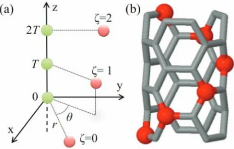
shown in Fig.1(a). The coordinates of the helical charges are described by
Xζ =RζX0+ζT, ζ = −∞, . . . ,+∞. (3)
a)Author to whom correspondence should be addressed. Electronic mail:
In the above equation, there is a charge located at position
X0=(rcosθ0,−rsinθ0, T0) in the ζ = 0 cell. There is a
singularity ifXcoincides with the position ofX0. The
sym-bolindicates that in this situation, the singular term from
ζ =0 is excluded from the summation. The basic helical op-eration is defined by a rotation of angleθ, described by the matrixR,
R=
⎛ ⎜ ⎝
cosθ −sinθ 0 sinθ cosθ 0
0 0 1
⎞ ⎟
⎠, (4)
coupled with a simultaneous translation by the axial vector
T=(0, 0,T), both oriented by convention with respect to the
z-axis.
The fundamental problem of evaluating the electrostatic field generated by discrete charges distributed in helical pat-terns is encountered in a number of areas of modern science. For example, in condensed matter physics, it is highly rel-evant for chiral charge-density waves5 and for
understand-ing the spin selective transport in helical molecular systems.6
In biological physics and soft matter, this problem is im-portant in understanding the relation between the helical structural and the generated local electric field,7–9 the
elec-trostatic interaction between biological helices,10,11 and the
electrostatic-driven helical patterns formed in fibers, nan-otubes, and pores.12 With the Green-function technique and
cylindrical and helical coordinates, analytical solutions have been derived. Unfortunately, these formulas are quite com-plex and appear less usable in practice, especially when they are expressed in terms of helical Bessel functions.13 Similar to the approach explored here, the electrostatic interaction be-tween discrete helices of charge with parallel axes have been examined based on truncated Fourier expansions of the dis-crete Coulomb sums.10
094110-2 Nikiforovet al. J. Chem. Phys.139, 094110 (2013)
FIG. 1. (a) Geometry for a discrete helical charge distribution. Charges on the helix at sitesζ=0, 1, 2 are shown in red, while compensating charges on the axis are green. (b) Example of a helical distribution of atoms in a boron nitride nanotube with one helix marked as red sites.
Direct numerical summations of the discrete Coulomb and dispersion sums are computationally inefficient and become intractable in the context of molecular dynamics and electronic structure calculations. For bulk systems with trans-lational symmetry, Ewald14 techniques15–17are currently uti-lized to evaluate such summations. These are mixed space ap-proaches based on the classical Ewald method presented in diverse textbooks.18,19 The short range contribution is
eval-uated in real space (where it decays rapidly) while the long range part is converted into a reciprocal space sum that is also fast converging. Originally proposed in three dimensions, the method has been generalized to one and two dimensions.20–23
Because objective MD renounces translational symmetry, none of these approaches are applicable here. Unfortunately, the utility of a helical Ewald approach has not been yet explored.
Our particular objective is to enable microscopic cal-culations in objective structures within the self-consistent charge (SCC) density-functional based tight-binding (DFTB) scheme.24 Note that the coupling of objective MD with the earlier two-center non-orthogonal TB and DFTB potentials25
(extended to capture dispersion forces within a cutoff ap-proximation), has already been achieved.26,27 This
non-SCC-DFTB objective MD methodology was successfully utilized to study homonuclear structures such as hexagonal, polycrys-talline, and screw-dislocated silicon nanowires,26,28 carbon
nanotubes,29–31graphene,32and graphene nanoribbons,33and
often produced compelling results. Unfortunately, the non-SCC-DFTB level of model is insufficient to tackle the rich variety of available helical nano- and bio-structures (for a re-cent review see Ref. 34) showing complex microscopic in-teractions, or for describing large mechanical deformations, or making credible predictions of new helical materials. The SCC-DFTB generalization is instead needed as it is more closely connected with first principles density functional the-ory (DFT) methods. As presented on several occasions,24,35,36
SCC-DFTB offers a superior description of chemical binding, especially in heteronuclear systems, while still being compu-tationally efficient enough to allow for dynamical simulations. Both aspects are important for objective MD simulations of complex structures. The SCC-DFTB description is superior
to force field approaches and, in fact, has even been used36as the high-level method in quantum mechanics/molecular me-chanics (QM/MM) simulations.
Unfortunately, evaluation of the aforementioned Coulomb sums on helices is a requirement for calculating the SCC-DFTB corrections in the objective MD framework. We approach this problem with the Ewald method general-ized to helical symmetry. In Sec. II we present the Ewald formulas for Coulomb and dispersion sums, and discuss their applicability with a numerical example. In Sec. III we briefly indicate how these formulas are then used in the SCC-DFTB formalism. The power of the resultant method is next illustrated with proof of concept self-consistent simulations of a boron-nitride (BN) nanotube, a zinc oxide (ZnO) nanowire containing a screw dislocation, and an ideal DNA molecule including van der Waals interactions. We highlight that all of the presented simulations are otherwise inaccessible to current methods without objective boundary conditions. SectionIVgives the conclusions.
II. THE HELICAL EWALD METHOD A. Coulomb sums
The approach investigated here is a direct generalization of the original Ewald method.14 To calculate the sum(1), we
use the identity
1
|X−Xζ|
= √1
π
∞
0
t−1/2exp(−|X−Xζ|2t)dt, (5)
obtained based on the integral representation of the gamma function.37Next, with the help of an adjustable Ewald param-eterη, we split the integration into long (VL) and short (VS) ranged terms
VL=
+∞
ζ=−∞
√1
π
η
0
t−1/2exp(−|X−Xζ|2t)dt (6)
and
VS=
+∞
ζ=−∞
√1
π
∞
η
t−1/2exp(−|X−Xζ|2t)dt. (7)
The distance between the observation point, X, and the location of charge, ζ, at Xζ =(rcos(ζ θ+θ0), −rsin (ζ θ
+θ0), ζ T +T0), is
|X−Xζ|2 =r2+r2−2rrcos (ζ θ+θ0−θ)
+(ζ T +T0−T)2. (8)
We focus first onVL. Concerning the angular term inθ, it is important to Fourier transform it as
e2rrcos(ζ θ+θ0−θ)t=
+∞
l=−∞
Il(2rrt)e−il(ζ θ+θ0−θ )
, (9)
where index l is an integer and Il is the modified Bessel
[image:3.612.59.291.51.199.2]one-dimension allows for39 +∞
ζ=−∞
e−t(ζ T+T0−T)2−ilζ θ
= +∞ k=−∞ +∞ −∞ e
−t(xT+T0−T)2e−i(lθ+2π k)xdx
= √ π T +∞ k=−∞
t−1/2e−i(lθ+2π k)T−TT0e− (lθ+2π k)2
4t T2 . (10)
Combining these results, the above integration was solved af-ter recognizing that it represents the Fourier transform of a Gaussian function. Thus,
VL= 1 T +∞ l=−∞ +∞ k=−∞
e−il(θ0−θ)e−i(lθ+2π k)T−TT0
×
η
0
t−1Il(2rrt)e−
(lθ+2π k)2
4t T2 −(r2+r2)tdt
−2
η
πδX0,X. (11)
The integral in the first term differs from the leaky aquifer function40 encountered when performing Ewald summation
in the pure one-dimensional case,21due to the presence of the
modified Bessel function. Notice also that the original Poisson formula still includes the ζ =0 term, regardless of the pos-sible singularity mentioned above. The last term in the above equation is needed in order to insure consistency with Eq.(6). The summation in Eq.(1)diverges because of the infinite extent of the helix. We remedy this by using the concept of a compensating background charge. The key point is that this divergence is due to thel=k=0 term of Eq.(11). We elimi-nate it by subtracting thek=0 term21(itself divergent) arising from an equispaced line of counter charges located along the
z-axis, starting at the origin and spaced at an interval ofT, as depicted in Fig.1(a). The corrected term then becomes
VlL=k=0= 1 T
η
0
t−1I0(2rrt)e−(r
2+r2)t
dt−1 T
η
0
t−1e−r2tdt.
(12)
The remaining term can be written as
Vl&kL =0 = 1 T +∞ l=−∞ +∞ k=−∞
e−il(θ0−θ)e−i(lθ+2π k)T−TT0
×
η
0
t−1Il(2rrt)e−
(lθ+2π k)2 4T2t −(r
2+r2)t
dt. (13)
To summarize, the long-ranged part of the electrostatic potential due to the helical charge distribution, less the back-ground term, is
VL=VlL=k=0+Vl&kL =0−2
η
πδX0,X. (14)
We treat theVSterm with an approach similar to the one
carried out for the one-dimensional lattice case.21 After
per-forming the change in variablesyζ = |X−Xζ|2tandy=r2t,
we obtain
VS =
+∞
ζ=−∞
√ 1
π|X−Xζ|
∞
η|X−Xζ|2
yζ−1/2exp(−yζ)dyζ
−1
T
+∞
ηr2
y−1e−ydy
=
+∞
ζ=−∞
(1/2, η|X−Xζ|2)
√
π|X−Xζ|
−(0, ηr2)
T . (15)
Here,is the incomplete gamma function. The second term after the equal sign is the remaining short-range background contribution from the neutralizing line of charge.
We now detail how the above approach is used in prac-tice. As stated before, under objective boundary conditions, we build the infinite structure not from translational unit cells, but from helical unit cells, Figs. 3(b), 4(b), and 5(b). The quantity of interest is the electrostatic potential at a given atomic site due to all other atoms in the infinite structure. To calculate it, we view the infinitely long structure as a collec-tion of infinitely long helices with a common axis – each in-dividual atom in the unit cell becomes a separate helix. For example, a (3,3) nanotube shown in Fig.1(b)is composed of six helices such as the one delineated with big (red) balls. To each helix we add one line of charges of opposite sign. As mentioned, these have a spacing of Tand lay on the z-axis, starting at the origin. Thus, the lines of counter-charges from each helix coincide geometrically. Assuming the unit cell is overall neutral, when the contributions from all of the helices are summed to obtain the electrostatic potential, the effect of the counter-charges cancels out. We revisit the neutralizing charges in Sec.III, where we show the expression for the elec-trostatic potential and provide a proof of the aforementioned cancellation.
B. Dispersion sums
To calculate the sum in Eq.(2), we use the identity
1
|X−Xζ|6 =
1 2
∞
0
t2exp(−|X−Xζ|2t)dt. (16)
As before, with the help of a controlling parameterη, we split Eq.(2)into long (WL) and short (WS) ranged components.
ForWLwe have
WL =
√ π 2T +∞ l=−∞ +∞ k=−∞
e−il(θ0−θ)e−i(lθ+2π k) T−T0
T
×
η
0
t3/2Il(2rrt)e−
(lθ+2π k)2
4t T2 −(r2+r2)tdt
−η3
6δX0,X. (17)
094110-4 Nikiforovet al. J. Chem. Phys.139, 094110 (2013)
RegardingWS, after performing the change in variables
yζ = |X−Xζ|2tandy=r2t, we obtain
WS=
+∞
ζ=−∞
1
2|X−Xζ|6
∞
η|X−Xζ|2
yζ2exp(−yζ)dyζ
= +∞
ζ=−∞
(3, η|X−Xζ|2)
2|X−Xζ|6
. (18)
C. Numerical example
It is not immediately obvious if the formulas presented above are numerically tractable and accurate in a truncated form, i.e., when indices|ζ|,|l|, and|k|are bounded byζmax, lmax, andkmax, respectively. The evaluation of the integral in
VL also introduces some complexity as it requires a
quadra-ture over the variablet, typically discretized asnnodes. We have implemented the Ewald formulas forV andW
as an independent Fortran module41 and explored the
appli-cability of the electrostatic sums for a simple numerical ex-ample. We use the geometry of the (3, 3) nanotube shown in Fig.1(b), on translating byT=1.42 Å alongzthe unit cell repeats with a rotation ofθ=60◦. To calculate the Ewald sum for the interaction of an atom with its helical images (such as the set of atoms highlighted in red in Fig.1(b)), we placeX
andX0on the surface of a tube of radius ofr=r=1.02 Å,
and setθ=θ0=T=T0=0.
The Ewald approach is robust since, when converged, the result will not depend on the specific value for the con-trolling parameter η. However, careful selection ofη is de-sirable for increasing the computational efficiency as the nu-merical approach is a balancing act between the cost of VL
andVSevaluations. Loweringηincreases theζ
maxthat needs
to be considered for the sum in VS, but decreases the l max, kmax, and n required for theVL term to converge. We find
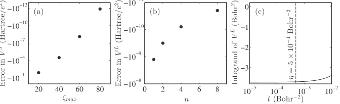
that the sum VS can be computed relatively quickly, and, as can be seen from Fig.2(a), converges approximately ex-ponentially with ζmax. The function evaluation and
numeri-cal integration (using a simple trapezoidal rule) involved in calculatingVL is more time-consuming and shows only an approximately power law convergence with the number of nodes (Fig.2(b)). Therefore, the optimal choice forηis small. So small as a matter of fact, thatVS is dominant enough to
be considered a first-order approximation to V. In this case
we find η = 5 × 10⁻⁴ bohr−2 provides the fastest
com-putational time, for which VS= −0.542 hartree/e2, while
VL= −0.0259 hartree/e2. Hereeis the electron charge.
We now examine the number of summation indices and numerical integration nodes required to achieve a precision greater than 10−10 hartree/e2. From Fig. 2(a)it can be seen thatζmax=80 is more than sufficient for this precision inVS.
Regarding VL, because the variable of integration tis kept small, the exponential factorexp(−(lθ+4T2π k)2t 2) in the integrand
of Eq.(13)decays extremely quickly withlθ +2πk. Thus,
|k|>0 terms almost never have to be considered, and|l|>0 terms do not have to be considered whenθ is large, such as in this example. Figure2(b)shows thatn=8 is sufficient to reach the desired accuracy. This is because the integrand of
VL is relatively flat in the interval of integration 0<t< η,
Fig. 2(c). The computational time required with these val-ues is nearly negligible,∼10 ms on a single core. The errors shown in Fig.2 are calculated with respect toVS evaluated
withζmax=160 andVLevaluated withn=1 000 000. These
quantities are converged to 10−15 hartree/e2 – doubling the
parameters produces identical results to that precision. As ex-pected, increasing (reducing)ηrequires a lower (higher) value ofζmaxin the evaluation ofVS, while increasing (decreasing) lmaxandnin evaluatingVL. The optimalηT2value increases
with decreasingr/Tandr/T.
Whenθ is small, however, thek=0 and |l|>0 terms ofVLneed to be also considered. Because the integrands be-come more non-linear, an increased number of nodes of in-tegration will be required. Thus, for smallθ, it is even more important to keepηsmall to reduce the computational effort of computingVL. This, in turn, would require more terms to
be considered in theVSsum.
III. SCC-DFTB UNDER OBJECTIVE BOUNDARY CONDITIONS
Encouraged by the above results, we used the developed module to couple SCC-DFTB to the helical symmetry. This represents the key step for developing the SCC-DFTB objec-tive MD capability.
Objective molecular structures2are structures consisting
of a finite or infinite set of identical cells (referred to as molecules), each cell having M atoms, in which the atomic environments of two corresponding atoms located in differ-ent cells can be mapped into each other by an orthogonal
FIG. 2. (a) Convergence ofVSwith increasingζ
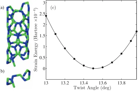
[image:5.612.51.302.50.176.2] [image:5.612.140.476.620.723.2]FIG. 3. SCC-DFTB simulation of intrinsic twist of (4, 2) BN nanotube. (a) Atomic structure and (b) objective computational domain containingM
=12 atoms. (c) Minimization of strain energy with respect to twist angle.
transformation, including the more complex helical transfor-mations. We consider an infinitely long structure extended in the z direction, where thejatom, located atXj,ζ in the cell
labeled by indexζ, can be mapped on the atom located atXj
in the reference cell using2
Xj,ζ =RζXj+ζT, j=1, . . . , M, −∞< ζ <∞. (19)
As before,Ris an axial rotational matrix of angleθandTthe axial vector of the helical transformation. In objective MD,1
only the atoms located in one cell are evolved in time un-der the objective boundary conditions, based on the objective structure formulas given by James.2 For example, the ideal
(4, 2) BN nanotube of Fig.3, objective simulations could be carried on the domain containing a finiteM=12 atoms placed under the boundary conditions provided by Eq.(19). Ideal val-ues forθ, andTcorresponding to the rolled-up construction can be obtained for any nanotube by following the approach detailed in Ref.43.
It is beyond the scope of this paper to review the two-center symmetry-adapted non-orthogonal TB and the well es-tablished SCC-DFTB. For the objective structures with heli-cal symmetry, the energy functional, Hamiltonian matrix ele-ments, and secular equations for the SCC-DFTB take similar forms to the standard periodic case. We therefore only indi-cate where Eqs.(1)and(2)enter into the machinery:
(i) Besides the usual band structure and short-ranged repulsive terms, the total energy in SCC-DFTB includes a Coulomb interaction between charge fluctuations,q, mea-sured with respect to the Mulliken charges of isolated neutral atoms. For an objective structure described by Eq. (19), the long-ranged part of this energy term, labeled E2nd, takes the
form
E2nd =
1 2
M
i=1
qiV(Xi). (20)
E2ndalso brings a contribution to the Hamiltonian matrix
ele-ments. This correction is of the form
iα|H2nd|jβ >=
1
2 < iα|jβ >[V(Xi)+V(Xj)], (21)
where|iα >and|jβ >are symmetry-adapted Bloch sums.26 Here i and j label atoms located in the computational cell, whileαandβ indicate orbital symmetries. At every “obser-vation point”Xi, the electrostatic potentialV(Xi) is generated
by the discrete chargesqj distributed overMideal helices,
one for each of theMatoms in the objective cell
V(Xi)= M
j=1
∞
ζ=−∞
qj
|Xi−Xj,ζ|
. (22)
Accurate evaluation is important since this correction term, Eq. (21), enters directly into the secular equation, which is central to SCC-DFTB. While in a neutral system the electro-static potential(22)is a well-defined and finite quantity, each individual helical sum over ζ arising from a single atom in the unit cell is divergent, as it represents an infinite number of particles of identical finite chargeqj. These divergences,
of course, cancel out to produce the finiteV(Xi). However in
practice one must compute each individual sum over ζ be-fore summing over j. Therefore, in our method, each indi-vidual helical sum is evaluated with the generalized Ewald formulas (14) and (15), where the divergences are elimi-nated with the help of the added neutralizing lines of charge. The neutralizing lines of charge cancel out when the individ-ual helical sums are combined, as illustrated in Figure 1 in the supplementary material41 and demonstrated in the next
paragraph.
We now show why the neutralizing lines of charges do not affect in the end the value ofV(Xi). When the
counter-charges are explicitly included, Eq. (1) becomes V(Xi)
=M j=1
∞
ζ=−∞qj(|X 1
i−Xj,ζ|−
1
|Xi−Xc,ζ|). Here, the
addi-tional term is the potential due to the infinite line of counter-charges Xc,ζ located on the z-axis at z =(− ∞, . . . ,−2T,
−T, 0, T, 2T, . . . , ∞). In our Ewald implementation, it is comprised of the latter terms of Eqs. (12) and (15). How-ever, since the locations of the counter-charges are identi-cal for each helix (independent of j), we can write V(Xi)
=M j=1
∞
ζ=−∞
qj
|Xi−Xj,ζ|−
∞
ζ=−∞|Xi−1Xc,ζ|
M
j=1qj. For
a neutral system,Mj=1qj is zero, thus the value ofV(Xi)
is not affected by the introduction of the counter-charges. (ii) The original DFTB has deficiencies in describing the long-ranged dispersion forces. To remedy this, a van der Waals term is added to the SCC-DFTB energy.27,44,45Its long range attractive component is
Edis= − M
i=1
W(Xi), (23)
where
W(Xi)= M
j=1
∞
ζ=−∞
C6ij
|Xi−Xj,ζ|6
. (24)
Here C6ij is the van der Waals coefficient between atomsi
andj.W(Xi) represents the attraction between atomiand the
atoms distributed over helices, labeled byj. It will be evalu-ated with Eqs.(17)and(18).
094110-6 Nikiforovet al. J. Chem. Phys.139, 094110 (2013)
unit cell with translational symmetry. (Tis simply the trans-lation component of the helical operation.) This important feature combined with the symmetry-adapted formulation of the Bloch sums26 ensures that SCC-DFTB objective MD can fully renounce translational symmetry in favor of a genuine helical geometry.
We find that the generalization to helical case of the clas-sical Ewald approach is pivotal for SCC-DFTB calculations under the boundary conditions of Eq. (19). The structural relaxations described next were carried out with a develop-mental version of the code DFTB+.42 The simulations were
considered converged when the magnitude of the maximum force on any atom was less than 1.0−4hartree/bohr.
A. Chiral BN nanotube
We first demonstrate the method for one-atom-thick het-eronuclear nanotubes. In this system we demonstrate the suit-ability of the proposed electrostatic approach when r ≈ r
and angle θ is relatively large. It is known that the compu-tational cost of chiral one-dimensional periodic systems, es-pecially when performed at a quantum mechanical level, is rather high as nanotubes can contain a large number of atoms in the periodic unit cell. The structure of nanotubes can be considered to be a rolled-up section of the planar sheet of the source material – for example, graphene in the case of car-bon nanotubes and a hexagonal boron-nitride mono-layer in the case of BN nanotubes. It has recently been obtained with non-SCC-DFTB objective MD that a general (n,m) nanotube can lose the translational periodicity predicted by this rolled-up construction due to a shear strain manifested as an intrinsic structural twist; for such cases, simulations relying on trans-lational symmetry would become even more demanding.43
The rich objective symmetry which characterizes this class of materials, however, can drastically reduce their com-putational costs, if adequately exploited. Following the screw-dislocation procedure described before29,43 we calculate the
optimal morphology of a (4, 2) BN nanotube, Fig. 3(a), using a computational cell consisting of six B–N dimers (12 atoms) positioned along the roll-up vector, Fig.3(b). The SCC treatment allows for better description of the partially ionic bonding in BN. We also used the most up to date DFTB parameters.46
In order to achieve a tolerance of<10−10 hartree in the
[image:7.612.314.559.142.253.2]electrostatic energy with this configuration, we use the nu-merical parameters and maximum summation indices listed in Table I, with the k-point grid chosen based on the ideas of Ref.47. The error is calculated by increasing the integra-tion nodes and maximum summaintegra-tion indices – the bare min-imum values required for this level of convergence are listed in parentheses. Starting with the ideal rolled-up configuration (modified to match each twist rate value we examine), we per-form conjugate-gradient relaxations. These calculations in-volved two stages: We first relax the atomic positions with fixed twist angleθ at constant T. Next, we optimize the NT parameterTfor these atomic coordinates, at the consideredθ. These simulations take only a few minutes each on a single core.
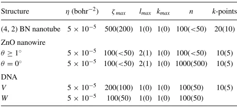
TABLE I. SCC-DFTB calculations under objective boundary conditions. Numerical parameters required to reach a tolerance of 10−10hartree in heli-cal Ewald summation of different structures and configurations considered. In order: Ewald split parameterη, maximum short-range summation index
ζmax, maximum long-range summation indiceslmaxandkmax, and number of nodesnused for numerical integration ofVL. Number ofk-points required
for energy convergence is also listed. Actual parameters used are listed first, bare minimum parameters required to reach required tolerance are listed in parentheses.
Structure η(bohr−2) ζ
max lmax kmax n k-points (4, 2) BN nanotube 5×10⁻⁵ 500(200) 1(0) 1(0) 100(<50) 20(10) ZnO nanowire
θ≥1◦ 5×10⁻⁵ 100(<50) 2(1) 1(0) 100(<50) 10(5) θ=0◦ 5×10⁻⁵ 100(<50) 2(1) 1(0) 1000(500) 10(5) DNA
V 5×10⁻⁵ 200(100) 1(0) 1(0) 100(50) 10(5)
W 5×10⁻⁵ 100(50) 1(0) 1(0) 100(50)
The net Mulliken charges on B and N atoms are found to be±0.366e. The energy due to the Coulomb part of the SCC correction is −0.438 hartree for the 12-atom unit cell. For comparison, we also evaluate this value using direct sum-mation. Over 4000 images in each direction are required to reach a tolerance of<10−10 hartree, a significantly increased
computational effort compared to the Ewald approach. The numerical values are equal up to this tolerance, demonstrat-ing the validity of the Ewald method. The total energy dif-ference due to the introduction of SCC corrections, including the Coulomb interaction, the short-range corrections, and the self-consistent adjustment of the wavefunction expansions, is
+0.0231 hartree.
The ideal roll-up construction predicts values forθandT
as 12.86◦/cell and 2.466 Å/cell, respectively. As can be seen in Fig.3(c), the untwisted (rolled-up) morphology does not correspond to a metastable state, in agreement with previ-ous predictions.43 The analogous non-SCC simulations
pre-dicts a twist angle of 13.51◦/cell and a length of 2.520 Å/cell. Our present simulation predicts a very similar twist angle of 13.52◦/cell, and a significantly differing (0.3% strain) length of 2.513 Å/cell.
B. Screw-dislocated ZnO nanowire
We now demonstrate the method in heteronuclear nanowires, when θ is small and r = r occurs. When a thin rod contains an axial screw dislocation, it becomes in-trinsically twisted.48Interestingly, all the experimentally
ob-served nanowires containing axial screw dislocations are also twisted.3With standard methods, one can efficiently simulate only ideal nanowires by considering their translational peri-odicity,T, and accounting for the small number of atoms,M, located in one primitive cell. The generated twist (unknown
FIG. 4. SCC-DFTB simulation of Eshelby twist of a ZnO nanowire. (a) Atomic structure and (b) objective computational domain containing
M=108 atoms. (c) Minimization of strain energy with respect to twist angle, showing an Eshelby twist of 6.61◦.
improved description of the binding by including the effects of electronic charge transfer from Zn to O.
We calculate the optimal length and twist of a ZnO nanowire of 8.53 Å radius extending along the [0001] direc-tion, Fig.4(a). The wire contains a centered axial screw dislo-cation, with the 5.4 Å minimum Burger’s vector allowable in ZnO. The simulation cell contains 108 atoms, the same as in the minimum translational cell of the wire, Fig.4(b). As be-fore, we require a tolerance of 10−10hartree, and the
numeri-cal Ewald parameters used are listed in TableI. The increased number of integration nodes required for the 0◦ case stems from the increased importance of the finite-lterms (herelmax
=1) at small angles. In general, because the integrand of the finite-lterms is more nonlinear, more nodes of integration are needed.
The simulations start with relaxed configurations previ-ously obtained with non-SCC-DFTB, or SCC results geomet-rically twisted to predict a configuration at a new angle (e.g., by applying the ideal geometric twist to the the simulation result at 1◦ to begin the 2◦ simulation). Each full conjugate-gradient relaxation took several hours (less than 10 h) on a single core.
The net charges on the Zn and O atoms range as±0.432– 0.575e. The total energy difference due to the introduction of SCC corrections is +1.07 hartree for the 108-atom unit cell. Our previous, non-SCC study of this structure predicted a twist angle of 6.71◦/cell and a length of 5.32 Å/cell.49The introduction of SCC changes these values to 6.61◦/cell and 5.28 Å/cell, respectively, Fig.4(c), confirming that these re-laxed structures and their amount of twist can be rationalized with Eshelby’s model.48
C. DNA strand
Finally, we demonstrate the simulation of heteronuclear biomolecules with this method, whenθis large andr=ris possible. Here, a larger number of atomic species is present and both the electrostatic and van der Waals sums are simul-taneously needed.
Biomolecules are perhaps the most obvious applica-tion for objective MD coupled with SCC-DFTB and
dis-persion. They often possess helical symmetry, and are al-most universally characterized by dispersion interactions. All biomolecules are heteronuclear, requiring the consideration of charge transfer for the most accurate description possible. As an emblematic example, here we consider an ideal single strand DNA.
Traditionally, DNA is simulated using either a cluster approximation or by PBC with the particle mesh Ewald method.51,52Both of these methods can be problematic.
Clus-ter simulations may introduce spurious end effects, and make the treatment of long strands of DNA computationally inten-sive. PBC overcomes these issues, but imposes translational symmetry constraints on the structure. Additionally, the num-ber of atoms in the PBC cell is large, and quantum treatments becomes less applicable. For this reason, simulations of DNA are typically carried out using empirical force-field models.51 The objective method carries none of these drawbacks. Segments of arbitrary length may be simulated as part of an infinite helix possessing arbitrary twist, allowing for study of sequence-dependent or general properties without end effects. Additionally, the objective simulations cells typically contain a small number of atoms, permitting the application of SCC-DFTB, which offers superior description of the interatomic interactions.
We have successfully carried out a series of calculations on a single strand DNA molecule – a helix comprised of adenosine nucleotides, Fig.5(a). The computational cell con-tains 33 atoms and comprises a single nucleotide, as shown in Fig. 5(b). Because DNA is a soft structure with many possible metastable configurations,51 we focus our demon-stration on the determination of the optimal twist angle at a fixed T = 3.38 Å. This is the typical value for the DNA B-type double helix, which was used as the starting config-uration for our single-helix simulation. The coordinates used are the default coordinates generated for the B-helix by the nablanguage.53–55Formerly, in order to apply PBC to a DNA
structure, investigators had to impose the constraint that there must be an integer number of nucleotides within one or a few 360◦turns of the helix. This artificial constraint runs contrary
FIG. 5. SCC-DFTB determination of optimal twist of a DNA molecule with
[image:8.612.315.559.539.684.2]094110-8 Nikiforovet al. J. Chem. Phys.139, 094110 (2013)
to the highly flexible and variable nature of the DNA con-figuration, and is not required here. The twist per single nu-cleotide is arbitrary and may represent a structure that pos-sesses no translational periodicity whatsoever.
The interatomic interactions involving elements P, O, N, C, H were described with the mio-1-1 parameter set.24,56We
continue to require an accuracy of 10−10 hartree, and the
values for both the V and W sums are shown in Table I. These simulations take several hours (less than 5) on a sin-gle core, implying also that SCC-DFTB calculations on larger objective cells (containing an integer multiple repeat of the 33 atom cell) should be tractable. We find an optimal twist of 33.27◦/cell, see Fig.5(c). Thus, our simulation predicts that the single helix differs significantly from the 36◦/cell twist angle typically associated with the B-double helix. Our opti-mized structure does not possess translational periodicity over any reasonable length. Its behavior deviates significantly from linear elasticity in the angle range we studied. This is to be ex-pected when such a soft material, with a complicated config-uration space, is placed under large strain. Thus, the quadratic fitting is restricted to the four points closest to the minimum. The torsional stiffness is 0.329 hartree Å. The P atom is the most positively charged with 1.23e, while the O atoms carry varying negative charges, as large as−0.62e. The other atoms are all closer to neutral. The total dispersion energy is+0.14 hartree for the 33-atom cell, while the total energy difference due to SCC corrections (not including dispersion) is of a sim-ilar value,+0.15 hartree.
IV. CONCLUSIONS
In this paper, we demonstrated that the generalization of the Ewald method to a helical geometry gives numerically tractable formulas for both the electrostatic potential and van der Waals energies. This approach provides an elegant and ro-bust way to incorporate helical symmetry into self-consistent treatments of the interatomic interactions, including SCC-DFTB and DFT. We successfully conduct proof of concept SCC-DFTB simulations under objective bounder conditions in charge-neutral heteronuclear nano- and bio-structures with various levels of complexity. Overall, objective MD benefits immensely from the coupling with SCC-DFTB as it increases the number and variety of objective structures which can be simulated with unprecedented accuracy. The scheme we pre-sented is for neutral systems only. It is further appealing to ex-plore the formulated expression for the Coulomb sum against the background provided by the neutralizing line of charge even in charged-cell objective calculations, to compute, for example, formation energies of charged defects in objective structures. The effect of the compensating line charges (which do not cancel out in that case) are still to be investigated.
ACKNOWLEDGMENTS
We acknowledge useful discussions with M. Elstner and A. Enyashin. Work supported by National Science Founda-tion (NSF) CAREER Grant No. CMMI-0747684, NSF Grant No. DMR-1006706, and NSF Grant No. CMMI-1332228.
T.D. acknowledges the hospitality of the guest program of MPI-PKS Dresden. Computations were performed at the Minnesota Supercomputing Institute.
1T. Dumitric˘a and R. D. James,J. Mech. Phys. Solids55, 2206 (2007). 2R. D. James,J. Mech. Phys. Solids54, 2354 (2006).
3S. Jin, M. J. Bierman, and S. A. Morin,J. Phys. Chem. Lett.1, 1472 (2010). 4See, for example, W. Falk and R. D. James,Phys. Rev. E73, 011917 (2006). 5J. Ishioka, Y. H. Liu, K. Shimatake, T. Kurosawa, K. Ichimura, Y. Toda, M.
Oda, and S. Tanda,Phys. Rev. Lett.105, 176401 (2010).
6R. Gutierrez, E. Diaz, R. Naaman, and G. Cuniberti,Phys. Rev. B 85, 081404(R) (2012).
7G. Edwards, D. Hochberg, and T. W. Kephart,Phys. Rev. E 50, R698 (1994).
8P. J. Lin-Chung and A. K. Rajagopal,Phys. Rev. E52, 901 (1995). 9D. Hochberg, G. Edwards, and T. W. Kephart, Phys. Rev. E55, 3765
(1997).
10J. Landy and J. Rudnick, Phys. Rev. E 81, 061918 (2010); e-print arXiv:0911.0192.
11A. A. Kornyshev and S. Leikin,J. Chem. Phys.107, 3656 (1997). 12F. J. Solis, G. Vernizzi, and M. O. de la Cruz,Soft Matter7, 1456 (2011). 13P. L. Overfelt,Phys. Rev. E64, 036603 (2001).
14P. P. Ewald,Ann. Phys.369, 253 (1921).
15N. Karasawa and W. A. Goddard III,J. Phys. Chem.93, 7320 (1989). 16F. G. Fumi and M. P. Tosi,Phys. Rev.117, 1466 (1960).
17D. E. Parry,Surf. Sci.49, 433 (1975); 54,195(1976).
18M. Born and K. Huang,Dynamical Theory of Crystal Lattices(Oxford University Press, Oxford, 1954).
19C. Kittel,Introduction to Solid State Physics(John Wiley & Sons, Inc., 1996).
20M. Porto,J. Phys. A33, 6211 (2000).
21D. J. Langridge, J. F. Hart, and S. Crampin,Comput. Phys. Commun.134, 78 (2001).
22A. Brodka and P. Sliwinski,J. Chem. Phys.120, 5518 (2004).
23O. N. Osychenko, G. E. Astrakharchik, and J. Boronat,Mol. Phys.110, 227 (2012).
24M. Elstner, D. Porezag, G. Jungnickel, J. Elsner, M. Haugk, T. Frauenheim, S. Suhai, and G. Seifert,Phys. Rev. B58, 7260 (1998).
25Th. Frauenheim, F. Weich, Th. Kohler, S. Uhlmann, D. Porezag, and G. Seifert,Phys. Rev. B52, 11492 (1995).
26D.-B. Zhang, M. Hua, and T. Dumitric˘a, J. Chem. Phys.128, 084104 (2008).
27A. Carlson and T. Dumitric˘a,Nanotechnology18, 065706 (2007). 28I. Nikiforov, D.-B. Zhang, and T. Dumitric˘a,J. Phys. Chem. Lett.2, 2544
(2011).
29D.-B. Zhang, R. D. James, and T. Dumitric˘a,J. Chem. Phys.130, 071101 (2009).
30D.-B. Zhang, R. D. James, and T. Dumitric˘a,Phys. Rev. B80, 115418 (2009).
31D.-B. Zhang and T. Dumitric˘a,ACS Nano4, 6966 (2010).
32D.-B. Zhang, E. Akatyeva, and T. Dumitric˘a,Phys. Rev. Lett.106, 255503 (2011).
33D.-B. Zhang and T. Dumitric˘a,Small7, 1023 (2011). 34M. Yang and N. A. Kotov,J. Mater. Chem.21, 6775 (2011).
35Th. Frauenheim, G. Seifert, M. Elstner, Z. Hajnal, G. Jungnickel, D. Porezag, S. Suhai, and R. Scholz,Phys. Status Solidi B217, 41 (2000). 36M. Elstner, Th. Frauenheim, and S. Suhai,J. Mol. Struct.: THEOCHEM
632, 29 (2003); M. Elstner,Theor. Chem. Acc.116, 316 (2006). 37Handbook of Mathematical Functions, edited by M. Abramowitz and I. A.
Stegun (Dover, New York, 1972), p. 255.
38E. Madelung, Die Mathematischen Hilfsmittel des Physikers(Springer, Berlin, 1950), p. 69.
39+∞
ζ=−∞f(ζ)=
+∞
k=−∞
∞
−∞f(x)e−2π ikxdx. Here f(ζ)
=e−t(ζ T+T0−T)2−ilζ θ. This formula is a specific case of the better known general Poisson summation formula,38 +∞
ζ=−∞f(x+ζ L)
= 1
L
+∞
k=−∞e2π ikx/L−∞∞ f(x)e−2π ikx/Ldx, withx=0 and periodicity L=1.
40F. E. Harris,J. Comput. Appl. Math.215, 260 (2008).
41See supplementary material athttp://dx.doi.org/10.1063/1.4819910for the helical Ewald module and the explanatory figure.
43D.-B. Zhang, E. Akatyeva, and T. Dumitric˘a,Phys. Rev. B84, 115431 (2011).
44M. Elstner, P. Hobza, T. Frauenheim, S. Suhai, and E. Kaxiras,J. Chem. Phys.114, 5149 (2001).
45L. Zhechkov, T. Heine, S. Patchkovskii, G. Seifert, and H. A. Duarte, J. Chem. Theory Comput.1, 841 (2005).
46B. Grundkötter-Stock, V. Bezugly, J. Kunstmann, G. Cuniberti, Th. Frauenheim, and Th. A. Niehaus,J. Chem. Theory Comput.8, 1153 (2012). 47H. J. Monkhorst and J. D. Pack,Phys. Rev. B13, 5188 (1976).
48J. D. Eshelby,J. Appl. Phys.24, 176 (1953).
49E. Akatyeva, L. Kou, I. Nikiforov, T. Frauenheim, and T. Dumitric˘a,ACS Nano6, 10042 (2012).
50E. Akatyeva and T. Dumitric˘a,Phys. Rev. Lett.109, 035501 (2012). 51A. Pérez, F. J. Luque, and M. Orozco,Acc. Chem. Res.45, 196 (2012). 52A. Noy and R. Golestanian,Phys. Rev. Lett.109, 228101 (2012). 53T. Macke and D. A. Case, inMolecular Modeling of Nucleic Acids, edited
by N. B. Leontes and J. SantaLucia, Jr. (American Chemical Society, Washington, DC, 1998), pp. 379–393.
54S. Arnott, P. J. Campbell Smith, and R. Chandraseharan, inHandbook of
Biochemistry and Molecular Biology, 3rd ed., Nucleic Acids Vol. II, edited by G. P. Fasman (CRC Press, Cleveland, OH, 1976), pp. 411–422. 55The code we used for coordinate generation can be found at
http://structure.usc.edu/make-na.