City, University of London Institutional Repository
Citation:
Assis, P. E. G. and Fring, A. (2009). From real fields to complex Calogero particles. Journal of Physics A: Mathematical and General, 42(42), doi: 10.1088/1751-8113/42/42/425206This is the unspecified version of the paper.
This version of the publication may differ from the final published
version.
Permanent repository link:
http://openaccess.city.ac.uk/772/Link to published version:
http://dx.doi.org/10.1088/1751-8113/42/42/425206Copyright and reuse: City Research Online aims to make research
outputs of City, University of London available to a wider audience.
Copyright and Moral Rights remain with the author(s) and/or copyright
holders. URLs from City Research Online may be freely distributed and
linked to.
City Research Online: http://openaccess.city.ac.uk/ [email protected]
arXiv:0907.1079v1 [hep-th] 6 Jul 2009
From real fields to complex Calogero particles
Paulo E. G. Assis and Andreas Fring
Centre for Mathematical Science, City University London, Northampton Square, London EC1V 0HB, UK
E-mail: [email protected], [email protected]
Abstract:We provide a novel procedure to obtain complexPT-symmetric multi-particle
Calogero systems. Instead of extending or deforming real Calogero systems, we explore here the possibilities for complex systems to arise from real nonlinear field equations. We exemplify this procedure for the Boussinesq equation and demonstrate how singularities in real valued wave solutions can be interpreted asN complex particles scattering amongst each other. We analyze this phenomenon in more detail for the two and three particle case. Particular attention is paid to the implemention of PT-symmetry for the complex multi-particle systems. New complexPT-symmetric Calogero systems together with their classical solutions are derived.
1. Introduction
The analytic continuation of real physical systems into the complex plane is a principle which has turned out to be very fruitful, since many new features can be revealed in this manner which might otherwise be undetected. A famous and already classical example, proposed more than half a century ago, is for instance Heisenberg’s programme of the analytic S-matrix [1]. Here our main concern will be complex multi-particle Calogero systems, in particular those exhibiting PT-symmetry [2].
Quantum systems are said to be PT-symmetric when they are invariant under si-multaneous parity P and time reversal T transformations. When the Hamiltonian, not necessarily Hermitian, exhibits this symmetry, i.e. [H,PT] = 0, and moreover when all wave-functions are also invariant under such an operation this property is referred to as unbroken PT-symmetry. The virtue of this feature is that it is a sufficient property to guarantee the spectrum of the Hamiltonian H to be real. The underlying mechanisms responsible for this are by now well understood [3, 4, 5, 6] and may be formulated al-ternatively in terms of pseudo/quasi-Hermiticity; for definitions see for instance [7] and references therein.
analytic S-matrix, and restrict to the real case in order to describe the underlying physics or alternatively one may try to give a direct physical meaning to the complex models.
With the latter motivation in mind complex PT-symmetric Calogero systems have been introduced and studied recently [8, 9, 10, 11, 12]. The hope for a direct physical interpretation stems from the fact that unbrokenPT-symmetry will guarantee their eigen-spectra to be real and allows for a consistent quantum mechanical description, i.e. such systems constitute well defined quantum systems which have been overlooked up to now. Nonetheless, so far any such proposal lacks a direct physical meaning and the complexi-fications are generally introduced in a rather ad hoc manner. Here our main purpose is to demonstrate that various complex Calogero models appear rather naturally from real valued nonlinear field equations and thus we provide a well defined physical origin for these systems.
The solutions for the real Calogero systems were found in the reverse order when compared to the usual way progress is made, i.e. the quantum theory was solved before the classical one. Calogero solved first the quantized one-dimensional three-body problem with pairwise inverse square interaction [13] and subsequently constructed the ground state of theN-body generalization [14] described by the Hamiltonian
HC = N
X
i=1
p2 i
2 + 1 2
N
X
i6=j
g
(xi−xj)2
, (1.1)
with g ∈ R being the coupling constant. Marchioro [15, 16] investigated thereafter the
classical analogue of these models obtaining a solution to which we will appeal below. The integrability of these classical counterparts was established later by Moser [17], using a Lax pair consisting of matrices L, M, with entries
Lij = piδij +
ı√g xi−xj
(1−δij), (1.2)
Mij = N
X
k6=i
ı√g
(xi−xk)2
δij−
ı√g
(xi−xj)2
(1−δij), (1.3)
constructed in such a manner that the Lax equation
dL
dt + [M, L] = 0 (1.4)
becomes equivalent to the Calogero equations of motion,
¨
xi = N
X
j6=i
2g
(xi−xj)3
. (1.5)
We use the notationı≡√−1 throughout the manuscript and abbreviate time derivatives as usual bydxi/dt= ˙xi andd2xi/dt2= ¨xi. Integrability follows in the standard fashion by
noting that all quantities of the for In = tr(Ln) /n are integrals of motion and conserved
Calogero systems have become very important in theoretical physics, having been explored in various contexts ranging from condensed matter physics to cosmology, e.g. [18, 19, 20]. The main focus of our interest here are the complex extensions which have been studied recently in connection withPT-symmetric models [8, 9, 10, 11, 12].
The idea of exploitingPT-symmetry in order to obtain models with real energies can be adapted to classical systems as well and has been used to formulate various complex extensions of nonlinear wave equations, such as the Korteweg-de Vries (KdV) and Burgers equations [21, 22, 23, 24]. In the classical case the reality of the energy is ensured in an even simpler way, as in that case thePT-symmetry of the Hamiltonian is sufficient. Remarkably these systems allow for the existence of solitons and compacton solutions [25, 26].
Here we shall explore PT-symmetry in a context where the complex extensions or deformations do not need to be imposed artificially, but instead we investigate whether this symmetry is already naturally present in the system, albeit hidden. To achieve this goal we exploit the fact that nonlinear equations, such as Benjamin-Ono and Boussinesq, can be associated to Calogero particle systems. We explore these connections and are then naturally led to complexPT-symmetric Calogero systems.
In the next section we shall demonstrate how a complex one-dimensionalPT-symmetric Calogero system is embedded in a real solitonic solution of the Benjamin-Ono wave equa-tion and how constrained PT-symmetric Calogero particles emerge from real solutions of the Boussinesq equation. Thereafter we construct the explicit solution of the three-particle configuration with the aforementioned constraint and show that the resulting motion, un-like in the unconstrained situation, cannot be restricted to the real line. We shall also establish that a subclass of this constrained Calogero motion is related to the poles in the solution of different nonlinear KdV-like differential equation. The relation of these com-plex particles with previously obtainedPT-symmetric complex extensions of the Calogero model [27] is discussed in section 5, where we demonstrate that they are different from those proposed here. Our conclusions are drawn in section 6.
2. Poles of nonlinear waves as interacting particles
The assumption of rational real valued functions as multi-soliton solutions of nonlinear wave equations was studied more than three decades ago by various authors, see e.g. [28]. We take some of these findings as a setting for the problem at hand. In order to illustrate the key idea we present what is probably the simplest scenario in which corpuscular objects emerge as poles of nonlinear waves, namely in the Burgers equation
ut+αuxx+β(u2)x= 0. (2.1)
Assuming that this equation admits rational solutions of the form
u(x, t) = 2α
β
N
X
i=1
1
x−xi(t)
it is straightforward to see that surprisingly theN poles interact with each other through a Coulombic inverse square force
¨
xi(t) =−2α N
X
j6=i
1 [xi(t)−xj(t)]2
. (2.3)
This pole structure survives even after making modifications in the ansatz for the wave equation, although the nature of the interaction may change. By acting on the second derivative in Burgers equation with a Hilbert transform
ˆ
Hu(x) = 1
πP V
Z +∞
−∞
dz u(z)
z−x, (2.4)
we obtain the Benjamin-Ono equation [29, 30]
ut+αHuˆ xx+β(u2)x = 0. (2.5)
As shown in [31], the ansatz proposed for the equation above which will allow for similar conclusions has a slightly different form,
u(x, t) = α
β
N
X
k=1
ı x−zk(t) −
ı x−z∗
k(t)
(2.6)
being, however, still a real valued solution with the only restriction that the complex poles satisfy complex Calogero equations of motion
¨
zk(t) = 8α2 N
X
k6=j
1 (zk(t)−zj(t))3
. (2.7)
Note that there is a difference in the power laws appearing in (2.3) and (2.7), but more importantly that equation (2.2) has real poles, whereas (2.6) has complex ones. We stress once more that the fieldu(x, t) is real in both cases. Hence, this viewpoint provides a nontrivial mechanism which leads to particle systems defined in the complex plane.
Interesting observations of this kind can be made for other nonlinear equations as well, but not always will the ansatz work directly, that is without any further requirements as in the previous cases. In some situations additional conditions might be necessary. Examples of nonlinear integrable wave equations for which such type of constraints occur are the KdV and the Boussinesq equations,
ut+ αuxx+βu2x= 0 and utt+ αuxx+βu2−γuxx = 0, (2.8)
respectively. For both of these equations one can have “N-soliton” solutions1 of the form
u(x, t) =−6α
β
N
X
k=1
1 (x−xk(t))2
, (2.9)
1
as long as in each case two sets of constraints are satisfied
˙
xk(t) =−12α N
X
j6=k
(xk(t)−xj(t))−2 , 0 = N
X
j6=k
(xk(t)−xj(t))−3, (2.10)
and
¨
xk(t) =−24α N
X
j6=k
(xk(t)−xj(t))−3 , x˙k(t)2= 12α N
X
j6=k
(xk(t)−xj(t))−2+γ, (2.11)
respectively. Naturally these constraints might be incompatible or admit no solution at all, in which case (2.9) would of course not constitute a solution for the wave equations (2.8). Notice that if thexk(t) are real or come in complex conjugate pairs the solution (2.9) for
the corresponding wave equations is still real.
Airault, McKean and Moser provided a general criterium, which allows us to view these equations from an entirely different perspective, namely to regard them as constrained multi-particle systems [28]:
Given a multi-particle Hamiltonian H(x1, ..., xN,x˙1, ...,x˙N) with flow xi = ∂H/∂x˙i
andx˙i=−∂H/∂xi together with conserved charges In in involution withH, i.e. vanishing
Poisson brackets {H, In} = 0, then the locus of grad(In) = 0 is invariant with respect to
time evolution. Thus it is permitted to restrict the flow to that locus provided it is not empty.
Taking the Hamiltonian to be the Calogero HamiltonianHC it is well known that one
may construct the corresponding conserved quantities from the Calogero Lax operator (1.2) as mentioned fromIn = tr(Ln)/n. The first of these charges is just the total momentum,
the next is the Hamltonian followed by non trivial ones
I1 = N
X
i=1
pi, I2=HC(g), I3 =
1 3
N
X
i=1
p3i +g
N
X
i6=j
pi+pj
(xi−xj)2
, . . . (2.12)
According to the above mentioned criterium we may therefore consider an I3-flow
restricted to the locus defined by grad(I2) = 0 or an I2-flow subject to the constraint
grad(I3−γI1) = 0. Remarkably it turns out that the former viewpoint corresponds exactly
to the set of equations (2.10), whereas the latter to (2.11) when we identify the coupling constant as g = −12α. Thus the solutions of the Boussinesq equation are related to the constrained Calogero Hamiltonian flow, whereas the KdV soliton solutions arise from an
I3-flow subject to constraining equations derived from the Calogero Hamiltonian.
As our main focus is on the Calogero Hamiltonian flow and its possible complexi-fications we shall concentrate on possible solutions of the systems (2.11) and investigate whether these type of equations allow for nontrivial solutions or whether they are empty. It will be instructive to commence by looking first at the unconstrained system. The classical solutions of a two-particle Calogero problem are given by
x1,2(t) = 2R(t)±
r
g
E + 4E(t−t0)
with E, t0 being initial conditions and ˙R(t) = 0 the centre of mass velocity. Relaxing this
condition by allowing boosts will only shifts the energy scale since the total momentum is conserved. Depending therefore on the initial conditions we may have either real or complex solutions.
The three particle model, i.e. taking N = 3 in (1.1), is slightly more complicated. Marchioro [15] found the general solution by expressing the dynamical variables in terms of Jacobi relative coordinates R, X, Y in polar form via the transformations R(t) = (x1(t)+x2(t)+x3(t))/3,X(t) =r(t) sinφ(t) = (x1(t)−x2(t))/√2 andY(t) =r(t) cosφ(t) =
(x1(t)+x2(t)−2x3(t))/
√
6. The variables may then be separated and the resulting equations are solved by
x1,2(t) = R(t) +
1
√
6r(t) cosφ(t)± 1
√
2r(t) sinφ(t), (2.14)
x3(t) = R(t)−
2
√
6r(t) cosφ(t), (2.15)
where
R(t) = R0+tR˜0 (2.16)
r(t) =
r
B2
E + 2E(t−t0)
2, (2.17)
φ(t) = 1 3cos
−1
(
ϕ0sin
"
sin−1(ϕ0cos 3φ0)−3 tan−1
√
2E
B (t−t0)
!#)
. (2.18)
The solutions involve 7 free parameters: The total energyE, the angular momentum type constant of motion B, the integration constants t0,φ0, R0, ˜R0 and the coupling constant
g, with the abbreviation ϕ0 = p
1−9g/2B2. We note that, depending on the choice of
these parameters, both real and complex solutions are admissible, a feature which might not hold for the Calogero system restricted to an invariant submanifold.
Let us now elaborate further on the connection between the field equations and the particle system and restrict the general solution (2.14)-(2.16) by switching on the additional constraints in (2.11) and subsequently study the effect on the soliton solutions of the nonlinear wave equation. Notice that the second constraint in (2.11) can be viewed as setting the difference between the kinetic and potential energy of each particle to a constant. Adding all of these equations we obtainHC =N γ/2, which provides a direct interpretation
of the constant γ in the Boussinesq equation as being proportional to the total energy of the Calogero model.
3. The motion of Boussinesq singularities
The two particle system, i.e.N = 2, is evidently the simplestI2-Calogero flow constrained
with grad(I3−γI1) = 0 as specified in (2.11). The solution for this system was already
provided in [28],
x1,2(t) =κ±
p
with κ,κ˜ taken to be real constants. In fact this solution is not very different from the unconstrained motion shown in the previous section (2.13). The restricted one may be obtained via an identification between the coupling constant and the parameter in the Boussinesq equation as κ = 2R(t), E = γ/4, ˜κ = t0 and g = −3α/4. The two soliton
solution for the Boussinesq equation (2.9) then acquires the form
u(x, t) =−12α
βγ
γ(x−κ)2+γ2(t−κ˜)2−3α
[γ(x−κ)2−γ2(t−˜κ)2+ 3α]2, (3.2)
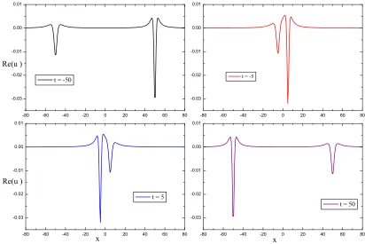
which, in principle, is still real-valued when keeping the constants to be real. When in-specting (3.2) it is easy to see that the two singularities repel each other on the x-axis as time evolves, thus mimicking a repulsive scattering process. However, we may change the overall behaviour substantially when we allow the integration constants to be complex, such that the singularities become regularized. In that case we observe a typical soli-tonic scattering behaviour, i.e. two wave packets keeping their overall shape while evolving in time and when passing though each other regaining their shape when the scattering process is finished, albeit with complex amplitude. A special type of complexification oc-curs when we take the integration constants κ,˜κ to be purely imaginary, in which case (3.2) becomes a solution for thePT-symmetrically constrained Boussinesq equation, with
PT : x → −x, t → −t, u → u. We depict the described behaviour in figure 1 for some special choices of the parameters.
-80 -60 -40 -20 0 20 40 60 80
-0.03 -0.02 -0.01 0.00 0.01
t = -5
-80 -60 -40 -20 0 20 40 60 80
-0.03 -0.02 -0.01 0.00 0.01
Re(u )
t = -50
-80 -60 -40 -20 0 20 40 60 80
-0.03 -0.02 -0.01 0.00 0.01
x
t = 50
-80 -60 -40 -20 0 20 40 60 80
-0.03 -0.02 -0.01 0.00 0.01
Re(u )
x
[image:8.612.102.514.404.679.2]t = 5
For larger numbers of particles the solutions have not been investigated and it is not even clear whether the locus of interest is empty or not. Let us therefore embark on solving this problem systematically. Unfortunately we can not simply imitate Marchioro’s method of separating variables as the additional constraints will destroy this possibility. However, we notice that (2.11) can be represented in a different way more suited for our purposes. Differentiating the second set of equations in (2.11) and making use of the first one, we arrive at the set of expressions
N
X
k6=j
( ˙xk(t) + ˙xj(t))
(xk(t)−xj(t))3
= 0, (3.3)
which are therefore consistency equations of the other two.
We now focus on the caseN = 3. Inspired by the general solution of the unconstrained three particle solution (2.14) and (2.15), we adopt an ansatz of the general form
x1,2(t) = A0(t) +A1(t)±A2(t), (3.4)
x3(t) = A0(t) +λA1(t), (3.5)
with Ai(t), i = 0,1,2 being some unknown functions and λ a free constant parameter.
We note that λ6= 1, since otherwise the three coordinates could be expressed in terms of only two linearly independent functions, A0(t) +A1(t) and A2(t), and we would not able
to express the normal mode like functions Ai(t) in terms of the original coordinates xi(t).
Calogero’s choice, λ=−2, in equation (2.15), allows an elegant map of Cartesian coordi-nates into Jacobi’s relative coordicoordi-nates, but other possibilities might be more convenient in the present situation. Here we keep λto be free for the time being.
Substituting this ansatz for the xi(t) into the second set of equations in (2.11) and
using the compatibility equation (3.3), we are led to six coupled first order differential equations for the unknown functionsA0(t), A1(t), A2(t)
( ˙A0(t) +λA˙1(t))2−γ
2g +
1 2A+(t)2
+ 1
2A−(t)2 = 0, (3.6)
( ˙A0(t) + ˙A1(t)±A˙2(t))2−γ
2g +
1 8A2(t)2
+ 1
2A∓(t)2 = 0, (3.7)
2 ˙A0(t) + (λ+ 1) ˙A1(t) + ˙A2(t)
A−(t)3 −
2 ˙A0(t) + (λ+ 1) ˙A1(t)−A˙2(t)
A+(t)3
= 0, (3.8)
˙
A0(t) + ˙A1(t)
4A2(t)3
+2 ˙A0(t) + (λ+ 1) ˙A1(t)±A˙2(t)
A∓(t)3 = 0. (3.9)
For convenience we made the identifications A±(t) =A2(t)±(λ−1)A1(t).
From the latter set of equations above, (3.8) and (3.9), we can now eliminate two of the first derivatives together with the use of the conservation of momentum. Depending on the choice, the remaining ˙Ai(t) are eliminated with the help of the first three equations
on A1(t) and A2(t). Subsequently we can expressA2(t), and consequently ˙A0(t),A˙1(t), in
terms ofA1(t) as the only unknown quantity. In this manner we arrive at
A2(t) =
p
−g−4γ(λ−1)2A
1(t)2
2√3γ , (3.10)
˙
A0(t) = √γ+
3g√γ(2 +λ) (λ−1)[g+ 16γ(λ−1)2A
1(t)2]
, (3.11)
˙
A1(t) =
9g√γ
(1−λ)[g+ 16γ(λ−1)2A
1(t)2]
, (3.12)
with g =−12α. This means that once we have solved the differential equation (3.12) for
A1(t) the complete solution is determined up to the integration of ˙A0(t) in (3.11) and a
simple substitution in (3.10). In other words we have reduced the problem to solve the set of coupled nonlinear equations (2.11) to solving one first order nonlinear equation.
Let us now make a comment on the number of free parameters, that is integration constants, occurring in this solution. In the original formulation of the problem we have started with 3 second order differential equations, so that we expect to have 6 integration constants for the determination ofx1, x2 and x3. However, together with the additional 3
constraining equations this number is reduced to 3 free parameters. Finally we can invoke the conservation of total momentum from (2.12), which yields 3 ¨A0(t) + (λ+ 2) ¨A1(t) = 0
and we are left with only 2 free parameters. We choose them here to be the two arbitrary constants attributed to the integration of ˙A0(t) in (3.11) and ˙A1(t) in (3.12), respectively.
In turn this also means that, without loss of generality, we may freely choose the constantλintroduced in (3.5). Indeed, keeping it generic we observe that the solutions for the Ai(t) do not depend on it despite its explicit presence in the equations (3.10), (3.11)
and (3.12). The most convenient choice is to take λ = −2 as in that case the equations simplify considerably.
Let us now solve (3.10), (3.11) and (3.12) and substitute the result into the original expressions (3.4) and (3.5) in order to see how the particles behave. We find
x1,2(t) = c0+√γt+ 1
12
g ξ(t)−
ξ(t)
γ
± ı
4√3
g ξ(t) +
ξ(t)
γ
, (3.13)
x3(t) = c0+√γt−
1 6
g ξ(t) −
ξ(t)
γ
, (3.14)
where for convenience we introduced the abbreviation
ξ(t) =
−54γ2(√γgt+c1) +
q
g3γ3+ [54γ2(√γgt+c
1)]2
13
. (3.15)
The above mentioned two freely choosable constants of integration are denoted byc0andc1.
As in the two particle case, we may once again compare this solution with the unconstrained one in (2.14), (2.15) when considering the Jacobi relative coordinates
R(t) =c0+t√γ, r2(t) =−
g
6γ and tanφ(t) =i
gγ+ξ2(t)
We observe that the solution is now constrained to a circle in the XY-plane with real radius whengγ∈R−. The values forφ(t) lead to the most dramatic consequence, namely
that the particles are now forced to move in the complex plane, unlike as in unconstrained Calogero system or the N = 2 case where all options are open.
Interestingly, despite the poles being complex, we may still have real wave solutions for the Boussinesq equation. Provided that ξ(t), γ, g, c0, c1 ∈Rthe pole x3(t) is obviously
real whereas x1(t) and x2(t) are complex conjugate to each other, such that the ansatz
(2.9) yields a real solution
u(x, t) = −6α
β
1
ϕ−16ξ(t)g −ξ(t)γ 2
+ (3.17)
+ 216α
β γ
2ξ(t)2
g2γ2−12gγ2ϕξ(t)−4γ(18γϕ2−g)ξ(t)2+ 12γϕξ(t)3+ξ(t)4 (g2γ2+ 6gγ2ϕξ(t) +γ(36γϕ2+g)ξ(t)2−6γϕξ(t)3+ξ(t)4)2
withϕ≡c0+√γt−x.
Due to the non-meromorphic form of ξ(t) it is not straightforward to determine how the solutions transforms under a PT-transformation. Nonetheless, the symmetry of the relevant combinations appearing in (3.13) and (3.14) can be analyzed well for c0, c1 ∈iR
andγ >0 . In that case the time reversal acts asT :ξ(t)g ±ξ(t)γ → ±ξ(t)g ±ξ(t)γ , which impliesPT :xi(t)→ −xi(t) fori= 1,2,3. Thus, the solutions to the constrained problem
are not only complex, but in addition they can also bePT-symmetric for certain choices of the constants involved.
4. Different types of constraints in nonlinear wave equations
It is clear from the above that the class of complex (PT-symmetric) multi-particle systems which might arise from nonlinear wave equations could be much larger. We shall demon-strate this by investigating one further simple example which was previously studied in [33] and also refer to the literature [32] for additional examples. One very easy nonlinear wave equations which, because of its simplicity, serves as a very instructive toy model is
ut+ux+u2 = 0. (4.1)
We may now proceed as above and seek for a suitable ansatz to solve this equation, possibly leading to some constraining equations in form a multi-particle systems. Making therefore a similar ansatz foru(x, t) as in (2.6) or (2.9) we take
u(x, t) =
N
X
i=1
1−z˙i(t)
x−zi(t)
. (4.2)
It is then easy to verify that this solves the nonlinear equation (4.1) provided thezi(t) obey
the constraints
¨
zi(t) = 2 N
X
j6=i
(1−z˙i(t))(1−z˙j(t))
zi(t)−zj(t)
We could now proceed as in the previous section and try to solve this differential equation, but in this case we may appeal to the general solution already provided in [33], where it was found that
u(x, t) = f(x−t)
1 +tf(x−t). (4.4)
solves (4.1) for any arbitrary function f(x) with initial condition u(x,0) = f(x). Com-paring (4.4) and (4.2) it is clear that the zi(t) can be interpreted as the poles in (4.4),
which becomes singular whenx→zi(t) =t+fi−1(−1/t), with i∈ {1, N}labeling the
dif-ferent branches which could result when assuming that f is invertible but not necessarily injectively. Making now the concrete choice for f to be rational of the form
f(x) =
N
X
i=1
ai
αi−x
, withαi, ai∈C, (4.5)
we can determine the poles concretely by inverting this function. First of all we obtain from the initial condition that
zi(0) =αi, z˙i(0) = 1 +ai and z¨i(0) = N
X
j6=i
2aiaj
αi−αj
. (4.6)
The first two conditions simply follow from the comparison of (4.4) and (4.2), but also follow, as so does the latter, from taking the appropriate limit in (4.5). We note that the total momentum is conserved for this systemPN
i=1z˙i(t) =N+PNi=1ai.
Let us now see how to obtain explicit expressions for the poles. Inverting (4.5) for
N = 2 it is easy to find that for generic values oft the poles take on the form
z1,2(t) =t+
¯
α12
2 +
¯
a12
2 t± 1 2
q
α2
12+ 2α12a12t+ ¯a212t2, (4.7)
where we introduced the notationαij =αi−αj, ¯αij =αi+αj and analogously for α→a.
We note that in the case N = 2 the constraint (4.3) can be changed into two-particle Calogero systems constraint with the identification g=a1a2α212.
Next we consider the caseN = 3 for which we obtain the solution
z1(t) = t−
a(t)
3 +s+(t) +s−(t) (4.8)
z2,3(t) = t−a(t)
3 −
1
2[s+(t) +s−(t)]±ı
√
3
2 [s+(t)−s−(t)], (4.9) where we abbreviated
s±(t) = hr(t)±pr2(t) +q3(t)i1/3, (4.10)
r(t) = 9a(t)b(t)−27c(t)−2a
3(t)
54 , q(t) =
3b(t)−a2(t)
9 , (4.11)
a(t) = −a1−α2−α3−t(a1+a2+a3), (4.12)
b(t) = α1α2+α2α3+α1α3+t[a1α¯23+a2α¯31+a3α¯21], (4.13)
In terms of Jacobi’s relative coordinates this becomes
R(t) =t−1
3a(t), r
2(t) = 6s
+(t)s−(t) and tanφ(t) =i
s−(t)−s+(t)
s−(t) +s+(t)
, (4.15)
which makes a direct comparison with the constrained Calogero system (3.16) straight-forward. As the system (4.8), (4.9) involves more free parameters than the constrained Calogero system (3.16), we expect to observe some relations between the parametersαi, ai
to produce the right number of free parameters. Indeed, we find that for
ai =−
g
2
Y
j6=i
(αi−αj)−2 (4.16)
and the additional constraints
c0 =
1 3
3
X
i=1
αi, c1=
2 27
Y
1≤j<k≤3 j,k6=l
(αj+αk−2αl), g= 4 3
X
i=1 i<j
αiαj−α2i, γ = 1. (4.17)
the two systems become identical. Thus we have obtained an identical singularity structure for two quite different nonlinear wave equations.
5. Complex Calogero models and PT-deformations
We have demonstrated in section 3 that the solutions of the constrained Calogero models are intrinsically of a complex nature. As there have been various proposals before in the literature suggesting complex Calogero systems in form of PT-symmetric deformations, we shall now compare them with the above outcome. We will argue that the deformations presented here are new and different to those suggested up to now.
The simplestPT-deformation of any model is obtained just by adding aPT-invariant term to the original Hamiltonian. For a many-body situation, this was proposed for the first time in the framework of An Calogero models by introducing the Hamiltonian [8]
H(q, p) =HC(q, p) + N
X
i6=j
ı˜gpi
(xi−xj)2
. (5.1)
In [10] it was shown that this simply corresponds to shifting the momenta in the standard Calogero Hamiltonian together with a re-definition of the coupling constant, which means the above construction is certainly quite different from the proposal (5.1).
The second type of deformation [12] consists of replacing directly the set ofℓ-dynamical variables q = {q1, . . . , qℓ} and their conjugate momenta p = {p1, . . . , pℓ} by means of a
[12]. Expanding the momenta as p = P
iκiαi, with κi ∈ R, this means for the Calogero
Hamiltonian
ε:HC(q, p)→HPT(˜q,p˜) =
1 2
X
i,j
κiκjα˜iα˜j +
1 2
X
˜ α∈∆˜
g
(˜α·q)2. (5.2)
In order to find the concrete forms for ˜q and ˜p we need to be more specific about the algebras involved. Let us therefore examine the models based on the rank 2 algebras A2,
B2 and G2. Depending on the dimensionality of the representation for the simple roots,
we obtain either a two or a three particle systems and may therefore compare with the solutions found in the previous sections. In all cases the deformations of the simple roots
α1 and α2 take on the general form
˜
α1(ε) =R(ε)α1+iI(ε)K12λ2, and α˜2(ε) =R(ε)α2−iI(ε)K21λ1, (5.3)
withλ1,λ2 being fundamental weights obeying 2λi·αj/α2j =δij, the functions R(ε),I(ε)
satisfy limε→0R(ǫ) = 1, limε→0I(ǫ) = 0 andKij = 2αi·αj/α2j are the entries of the Cartan
matrix. Let us now take the following two dimensional representations for the simple roots and fundamental weights
A2 : α1= (1,−√3), α2 = (1,√3), λ1 = 32α1+13α2, λ2= 13α1+23α2,
B2 : α1= (1,−1), α2 = (0,1), λ1 =α1+α2, λ2= 12α1+α2,
G2: α1= (−
q
3
2,
q
1
2), α2 = (
√
6,0), λ1 = 3α1+α2, λ2= 3α1+ 2α2.
(5.4)
We easily verify that this reproduces the correct entries for the Cartan matrices A2 :
K11 = K22 = 2, K12 = K21 = −1, B2 : K11 = K22 = 2, K12/2 = K21 = −1 and
G2 : K11 = K22 = 2, K12 = K21/3 = −1. Having constructed the deformed roots we
compute next the deformed conjugate momenta and coordinates. In the representations (5.4) the kinetic energy term changes just by an overall factor as
˜
p2 =
R(ε)−ν2gI(ε)
p2 withνA2 = 1/ √
3, νB2 = 1, νG2 =− √
3. (5.5)
The specific choice R(ε) = coshε and I(ε) = ν−2
g sinhε, used in [12], keeps the kinetic
energy term completely invariant, in the sense that the original and deformed momenta are identical. The dual canonical coordinates ˜q are computed from
˜
α·q = ˜q·α, α, q∈R, ˜α,q˜∈R⊕iR. (5.6)
We find
˜
q1 =R(ε)q1+iνgI(ε)q2, and q˜2 =R(ε)q2−iνgI(ε)q1. (5.7)
We will now argue that (5.7) is always different from the constrained two particle solution of the Calogero model (3.1). In order to see this we recall first of all that for the solution to be PT-symmetric we require κ,κ˜ ∈ iR. Equating now the sums x1 +x2 = ˜q1+ ˜q2 we
conclude that q1(t) = −q2(t) = −κ/νgI(ε) = const. Next we compute (x1−x2)2, which
yields
This equation is inconsistent as the right had side is real and time independent, a condition which can not be achieved for the left hand side. This proves our statement that the deformation method suggested here is genuinely different from the proposal in [12] in the two particle case.
Keeping the deformed roots to be of the form (5.3), the three dimensional repesenta-tions for the simple roots
A2:α1 = (1,−1,0), α2 = (0,1,−1), G2 :α1= (1,−1,0), α2 = (−2,1,1), (5.9)
yield the same result for the kinetic energy term (5.5), but obviously have to produce different dual canonical coordinates ˜q. In this case we obtain
˜
q1 = R(ε)q1+iζgI(ε)(q2−q3), (5.10)
˜
q2 = R(ε)q2+iζgI(ε)(q3−q1), (5.11)
˜
q3 = R(ε)q3+iζgI(ε)(q1−q2), (5.12)
where ζA2 = 1/3 andζG2 =−1. Equating these solutions with (3.13), (3.14) and solving
the resulting equations for the qi with i= 1,2,3, it is easy to argue that theqi can not be
made real, which establishes the claim that the solutions are also intrisically different for the three particle model.
6. Conclusions
Hitherto there have been two different types of procedures to complexify Calogero models. As explained in section 5 one may either addPT-symmetric terms to the original Hamilto-nian [8], which have turned out to be simple shifts in the momenta [10] or one may directly deform the root system on which the formulation of the model is based [12]. In all these approaches the deformation is introduced in a rather ad hoc fashion. In this paper we have provided a novel mechanism, which has real solutions of physically motivated nonlinear wave equations as the starting point. The constrained motion of some solitonic solutions of these models then led to complex Calogero models, some of them beingPT-symmetric. There are some obvious open problems left. For instance it would naturally be very interesting to study systems involving larger numbers of particles, which would correspond to higher soliton solutions for the nonlinear wave equations. Clearly the study of differ-ent types of wave equations, such as the KdV etc and their PT-symmetrically deformed versions would complete the understanding.
(2.8 )
(2.13 ),(3.1 ) (2.13 ),(3.1 )
(2.3 ) (2.1 ) unconstrained
( 2.11 )
c ons
tra ine
d ( 2.8 )
,( 4.1 )
( 2.7 )
unc ons
tra ine
d ( 2.5 )
complex nonlinear field equations real nonlinear field equations
complex multi-particle systems real multi-particle systems
Acknowledgements: P.E.G.A. is supported by a City University London studentship.
We are grateful to Monique Smith for useful discussions.
References
[1] W. Heisenberg, Quantum theory of fields and elementary particles, Rev. Mod. Phys.29 (1957) 269–278.
[2] C. M. Bender and S. Boettcher, Real Spectra in Non-Hermitian Hamiltonians HavingPT
Symmetry, Phys. Rev. Lett. 80(1998) 5243–5246.
[3] E. Wigner, Normal Form of Antiunitary Operators, J. Math. Phys.1(1960) 409–413.
[4] C. F. M. Faria and A. Fring, Non-Hermitian Hamiltonians with real eigenvalues coupled to electric fields: From the time-independent to the time-dependent quantum mechanical formulation, Laser Physics17 (2007) 424–437.
[5] C. M. Bender, Making sense of non-Hermitian Hamiltonians, Rept. Prog. Phys.70(2007) 947–1018.
[6] A. Mostafazadeh, Pseudo-Hermitian Quantum Mechanics, arXiv:0810.5643.
[7] P. E. G. Assis and A. Fring, Non-Hermitian Hamiltonians of Lie algebraic type, J. Phys. A 42 (2009) 015203(23).
[8] B. Basu-Mallick and A. Kundu, Exact solution to the Calogero model with competing long-range interactions, Phys. Rev. B 62(2000) 9927–9930.
[9] M. Znojil and M. Tater, Complex Calogero model with real energies, J. Phys. A 34(2001) 1793–1803.
[11] S. R. Jain, Random matrix theories and exactly solvable models, Czech. J. Phys.56(2006) 1021–1032.
[12] A. Fring and M. Znojil, PT-symmetric deformations of Calogero models, J. Phys. A41 (2008) 194010(17).
[13] F. Calogero, Solution of a Three-Body Problem in One Dimension, J. Math. Phys.10(1969) 2191-2196.
[14] F. Calogero, Ground State of a One-DimensionalN-Body System, J. Math. Phys.10(1969) 2197–2200.
[15] C. Marchioro, Solution of a Three-Body Scattering Problem in One Dimension, J. Math. Phys.11 (1970) 2193–2196.
[16] F. Calogero and C. Marchioro, Exact solution of a one-dimensional three-body scattering problem with two-body and/or three-body inverse-square potentials, J. Math. Phys.15 (1974) 1425–1430.
[17] J. Moser, Three Integrable Hamiltonian Systems Connected with Isospectral Deformations, Advances in Mathematics 16(1975) 197–220.
[18] J. Avan and M. Talon, Classical R-matrix structure for the Calogero model, Phys. Lett. B 303(1993) 33–37.
[19] H. Azuma and S. Iso, Explicit relation of the quantum Hall effect and the Calogero-Sutherland model, Phys. Lett. B 331(1994) 107-113.
[20] G. W. Gibbons and P. K. Townsend, Black holes and Calogero models, Phys. Lett. B454 (1999) 187–192.
[21] C. M. Bender and J. Feinberg, Does the complex deformation of the Riemann equation exhibit shocks?, J. Phys. A 41, (2008) 244004(8).
[22] C. M. Bender, D. C. Brody, J. Chen and E. Furlan, PT-symmetric extension of the Korteweg-de Vries equation, J. Phys. A 40, (2007) F153–F160.
[23] A. Fring, PT-symmetric deformations of the Korteweg-de Vries Equation, J. Phys. A40, (2007) 4215–4224.
[24] P. E. G. Assis and A. Fring, Integrable models from PT-symmetric deformations, J. Phys. A. 42, (2009) 105206(12).
[25] C. Bender, F. Cooper, A. Khare, B. Mihaila and A. Saxena, Compactons inPT-symmetric generalized Korteweg-de Vries Equations, arXiv.org:0810.3460
[26] P. E. G. Assis and A. Fring, Compactons versus Solitons, arXiv:0901.1267.
[27] A. Fring, Particles versus fields inPT-symmetrically deformed integrable systems, arXiv:0903.4670, to appear in Pramana J. Phys.
[28] H. Airault, H. P. McKean and J. Moser, Rational and Elliptic Solutions of the Korteweg-de Vries Equation and a Related Many-Body Problem, Comm. pure appl. Math. 30(1977) 95–148.
[29] T. B. Benjamin, Internal waves of permanent form in fluids of great depth, J. Fluid Mech. 29 (1967) 559–592.
[31] H. H. Chen, Y. C. Lee and N. R. Pereira, Algebraic internal wave solutions and the integrable Calogero-Moser-SutherlandN-body problem, Phys. Fluid22(1979) 187–188.
[32] J. J. Nimmo and S. N. M. Ruijsenaars, Tzitzeica solitons vs. relativistic Calogero-Moser 3-body clusters, arXiv:0903.2131.