Forecasting with Medium and Large Bayesian VARS

(1)

S

TRATHCLYDE

D

ISCUSSION

P

APERS IN

E

CONOMICS

D

EPARTMENT OF

E

CONOMICS

U

NIVERSITY OF

S

TRATHCLYDE

G

LASGOW

FORECASTING WITH MEDIUM AND LARGE BAYESIAN

VARS

B

Y

GARY

KOOP

(2)

Forecasting with Medium and Large Bayesian VARs

Gary Koop

University of Strathclyde

February 2010

Abstract

This paper is motivated by the recent interest in the use of Bayesian VARs for forecasting, even in cases where the number of dependent variables is large. In such cases, factor methods have been traditionally used but recent work using a particular prior suggests that Bayesian VAR methods can forecast better. In this paper, we consider a range of alternative priors which have been used with small VARs, discuss the issues which arise when they are used with medium and large VARs and examine their forecast performance using a US macroeconomic data set containing 168 variables. We …nd that Bayesian VARs do tend to forecast better than factor methods and provide an extensive comparison of the strengths and weaknesses of various approaches. Our empirical results show the importance of using forecast metrics which use the entire predictive density, instead of using only point forecasts.

Keywords: Bayesian, Minnesota prior, stochastic search variable selection, predictive likelihood

Acknowledgements: I would like to thank Dimitris Korobilis for helpful discussions. Some of the Matlab programs used in this paper are extensions of the ones available on our website:

(3)

1 Introduction

Vector autoregressive (VAR) models have a long and successful tradition in the fore-casting literature (e.g. Doan, Litterman and Sims, 1984 and Litterman, 1986). VARs are parameter-rich models and shrinkage of various sorts has been found to greatly improve forecast performance. Bayesian methods have proved popular since the use of prior information o¤ers a formal way of shrinking forecasts. Almost all of the existing literature focusses on VARs where the number of dependent variables is small (typically two or three and rarely more than ten). However, in a recent paper, Banbura, Gian-none and Reichlin (2010), hereafter BGR, consider larger Bayesian VARs. They work with what they call a “medium” VAR involving 20 dependent variables and a “large” VAR with 130 dependent variables. Traditionally, researchers working with so many macroeconomic variables have used factor methods (e.g. Stock and Watson, 2002, 2006, Forni, Hallin, Lippi and Reichlin, 2003, Koop and Potter, 2004 and Korobilis, 2009). However, BGR …nds that medium and large Bayesian VARs can forecast better than factor methods (at least in their empirical application). Given that VARs have other advantages (e.g. in that impulse responses are easier to interpret), this suggests Bayesian VARs could be a useful addition to the macroeconomic forecaster’s toolbox even in cases where the research is working with dozens or hundreds of variables.

BGR uses a natural conjugate variant of the Minnesota prior popularized by Doan, Litterman and Sims, 1984 and Litterman, 1986. The BGR prior shrinks all VAR co-e¢ cients towards zero except for coco-e¢ cients on own lags of each dependent variable. The latter are either set to one (for variables which exhibit substantial persistence) or zero (for variables which do not). Thus, forecasts are shrunk towards a random walk for some variables and towards white noise for others. The degree of shrinkage is con-trolled by a single scalar hyperparameter. This is potentially an attractive and simple way of doing Bayesian shrinkage in large VARs. However, there are alternative ways of implementing the Minnesota prior which allow for di¤erent degrees of shrinkage on coe¢ cients (e.g. coe¢ cients on own lags of a dependent variable can be shrunk to a lesser extent than coe¢ cients on lags of other dependent variables). Such methods are more restrictive in their treatment of the error covariance matrix than BGR’s imple-mentation of the Minnesota prior. Nevertheless it is possible that allowing for di¤erent degrees of shrinkage provides bene…ts which outweigh the costs of such restrictiveness. A …rst purpose of this paper is to investigate this issue.

(4)

dependent variables.

A third purpose of this paper is to develop methods for combining the Minnesota prior with the SSVS prior. After all, each of them has attractive properties and so it is possible that a combination of the two will improve forecast performance.

Finally, the Bayesian methods used in this paper produce an entire predictive dis-tribution and not merely a point forecast. The previous literature (e.g. BGR and Mar-cellino, Stock and Watson, 2006) typically focusses on point forecasts, using measures of forecast performance such as mean squared forecast error (MSFE). In this paper, the list of forecast metrics is expanded to include a measure based on the predictive likelihood which involve the entire predictive distribution.

The data set used in this paper is an updated version of that used in Stock and Watson (2008) and is described in the Data Appendix.1 The complete data set include 168 variables and runs from 1959Q1 through 2008Q4. Our forecasting exercise …nds that Bayesian VAR methods do out-perform factor methods. However, we …nd no single approach to Bayesian VAR forecasting consistently forecasts best. Roughly speaking, we …nd that SSVS-based methods work best in cases where relatively low dimensional VARs are adequate, but approaches based on the Minnesota prior work best when medium or large VARs are needed. But there are some important exceptions to this pattern. Furthermore, traditional, simpler implementations of Minnesota priors often out-perform BGR’s version of the Minnesota prior. Our results highlight the di¤erent ways in which di¤erent priors achieve the shrinkage and/or parsimony that is important in achieving good forecast performance with large macroeconomic data sets.

2 The Econometrics of Bayesian VARs

We write the VAR in matrix form as:

Y =XA+"; (1)

whereY is a T n matrix with tth _{row given by}_y0

twhere yt is a vector of n dependent

variables, X is a T K matrix. In our empirical work K = (1 +pn) since each row of contains p lags of each dependent variable and an intercept. That is, the tth row of

X is given by the vector 1; y0

t 1; : : : ; yt p0 . A is the matrix of coe¢ cients and " is a

T n matrix withtth_{row given by}_"0

t. "tare independentN(0; )errors fort= 1; ::; T.

De…ne =vec(A) which is a vector ofnK elements. The dimensionality of plays a key role in the following discussion. Note that a large VAR with quarterly data might haven = 100 and p= 4 in which case contains over40;000 elements. With monthly data it would have over 100;000 elements. For a medium VAR, might have about

1;500 elements with quarterly data. , too, will be parameter rich, containing n(n₂+1) elements. A typical macroeconomic quarterly data set might have approximately two hundred observations and, hence, the number of coe¢ cients will far exceed the num-ber of observations. Bayesian methods combine likelihood function with prior. It is well-known (e.g. Poirier, 1998) that, even if some parameters are not identi…ed in the likelihood function, under weak conditions the use of a proper prior will lead to a valid posterior density and, thus, Bayesian inference is possible. However, prior information

(5)

becomes increasingly important as the number of parameters increases relative to sam-ple size. A theme of this paper is to investigate the role of prior information as it relates to how shrinkage is done.

2.1 Natural conjugate priors for VARs

For reasons to be made clear in this sub-section, BGR work with a natural conjugate prior,2 despite the fact that there is a well-known drawback with the use of such priors with VARs (see, e.g., Kadiyala and Karlsson, 1997). The natural conjugate prior has the form:

j N( ; V) (2)

and

1 _{W S} 1_; ₍₃₎

where ; V ; and S are prior hyperparameters and W S 1; denotes the Wishart distribution with scale S 1 and degrees of freedom . For future reference, let A be a

K n matrix de…ned through the relationship =vec(A).

Note that the traditional Minnesota prior is not the same as this natural conjugate prior since the former does not treat as a matrix of unknown parameters, but simply replaces with an estimate, b. In particular, the traditional Minnesota prior assumes to be a diagonal matrix with diagonal elements s2_i where s2_i is the standard OLS estimate of the error variance in an AR(p) model for the ith _{variable. Sensibly wishing}

to allow for correlations between the errors, BGR treats as an unknown positive de…nite matrix with S chosen in a manner inspired by the Minnesota prior.

Natural conjugate priors can be interpreted as arising from a …ctitious prior data set. To be precise, if Y and X are(K+n) n and (K+n) K, respectively, then we can write the prior hyperparameters as ,

A= (X0X) 1X0Y ;

S = (Y XA)0(Y XA)

and

V = (X0X) 1:

If we stack the prior and actual data as Y = (Y0_{; Y}0₎0 _and _X _{= (}_X₀_{; X}0₎0_{, it can be}

shown that the posterior is:

j ; Y N ; V (4)

and

1

jY W S 1; (5)

where

2_{Natural conjugate priors are those where the prior, likelihood and posterior come from the same}

(6)

V = X0X 1; (6)

A= X0X

1

X0Y ;

=vec A ,

S= Y XA 0 Y XA

and

=T + :

The general form for the prior “sample” is

Y = V

1 2A

S12

!

; X = V

1 2

0n nK

; (7)

where notation such as S12 implies a matrix such that S 1 2

0

S12 = S and 0

a b is an

a b matrix of zeros.

BGR show how a prior which coincides with the traditional Minnesota prior (except that is treated as unknown and a single scalar is used for shrinkage instead of the two scalars used for shrinkage in the traditional implementation) arises if the …ctitious sample is set as:

Y =

0 @

diag( 1s1;::; nsn) 0(np n+1) n

diag(s1; ::; sn) 1

A; X =

0 @ Jp

diag(s1;::;sn)

0np 1

01 np v

0n np 0n 1

1

A; (8)

whereJp =diag(1;2; ::; p); diag(:)denotes a diagonal matrix. i = 1if theith variable

is believed to exhibit substantial persistence (i.e. it ensures shrinkage towards a random walk) and i = 0 if theithvariable is believed to exhibit little persistence (i.e. it ensures

shrinkage towards white noise). The middle row of X determines the prior for the intercept. By choosing v to be very small, a relatively noninformative prior for the intercept is obtained. The form of Y implies the prior mean for the intercept is zero.

Posterior inference about the VAR coe¢ cients can be carried out using the fact that the marginal posterior (i.e. after integrating out ) for is a multivariate t-distribution. The mean of this t-distribution is , its degrees of freedom parameter is

and its covariance matrix is:

var( _jY) = 1

n 1S V :

The predictive distribution for yT+1 in this model has an analytical form and, in

particular, is multivariate-t with degrees of freedom. Point forecasts can be based on the predictive mean:

E(yT+1jY) = xT+1A

0

:

(7)

var(yT+1jY) =

1

2 1 +xT+1V x 0

T+1 S:

When forecasting more than one period ahead, an analytical formula for the predic-tive density does not exist. This means that either the direct forecasting method must be used (which turns the problem into one which only involves one step ahead forecast-ing) or predictive simulation is required. In this paper, we use the direct method.

The use of the natural conjugate prior leads to one large bene…t: analytical results are available for Bayesian inference and forecasting, so no posterior simulation is required. For large Bayesian VARs a second bene…t exists: the V form for the conditional posterior covariance matrix of in (4) enormously simpli…es computation. Note that with this prior, calculatingV involves inverting aK K matrix (see 6) which, even for a large VAR (when K is a few hundreds or, at most, a few thousand) is feasible. To preview one of the crucial econometric issues in the present paper, when working with non-conjugate priors such as the conventional implementation of SSVS, calculating the posterior covariance matrix involves inverting annK nK matrix (e.g. with quarterly data it would involve inverting something like a 40;000 40;000 matrix). For medium VARs (e.g. up to n = 20), Bayesian computation with non-conjugate priors is feasible (but very slow), with large VARs it is computationally infeasible. It is this consideration which leads us to investigate the conditionally conjugate implementation of SSVS for VARs discussed below.

However, the natural conjugate prior has a restrictive property which means it has been rarely used in practice. This arises from the fact that the prior covariance of the coe¢ cients in equationiis iiV where iiis the(ii)th element of (see 2). This implies

that the prior variance of the coe¢ cients in any two equations must be proportional to one another, a possibly restrictive feature. The traditional Minnesota prior (which treats as …xed) has the property that coe¢ cients on own lags (i.e. in equationithese are lags of the ith _{dependent variable) have a larger prior variance (i.e. are shrunk less)}

than coe¢ cients on other lags (i.e. lags of the dependent variables in other equations). This feature is not possible using the natural conjugate prior and, accordingly, BGR applies the same degree of shrinkage to coe¢ cients on own and other lags. In an ideal world, one may wish to relax such an assumption and this is something we investigate below. But given computational limitations and the inevitable compromises and trade-o¤s of empirical work in high-dimensional models, it may be a sensible one to make.

However, it is worth investigating whether having two prior hyperparameters con-trolling shrinkage ( 1 and 2) as in the original Minnesota prior yields forecasting

(8)

are the ones labelled “Three Main Variables used in all VARs” in the Data Appendix. This approach allows for correlation between the errors in the most important equa-tions in the VAR. This may represent a good compromise between the two extremes of allowing no correlation between any errors (as in the original Minnesota prior) and the other extreme of allowing for correlation between all of the errors (as in BGR) and running the risks associated with over-parameterization.

2.2 The Non-conjugate SSVS Prior

The variant of the Minnesota prior used in BGR has many advantages (e.g. the fact that analytical results exist for posterior and predictive density). However, it does embody some quite extreme prior assumptions. For instance, the huge[n (1 +pn)] [n (1 +pn)]prior covariance matrix for has a prior which is parameterized extremely tightly in terms of a single scalar with most elements simply being set to zero. It is also a data-based prior withs2

i being chosen based on preliminary estimation of AR(p)

models for each variable. Furthermore, the prior will take the same form at each point in time in a recursive forecasting exercise and so coe¢ cients will be shrunk in the same way at all points in time. This may be inappropriate if the set of relevant predictors for a dependent variable changes over time, or if the persistence in a dependent variable changes over time. The SSVS prior is an alternative method of achieving shrinkage in VARs, but it does so in a di¤erent manner and without so many restrictive assumptions. And the SSVS prior can adapt by including/excluding di¤erent explanatory variables as time goes by in a recursive or rolling forecasting exercise.

To explain the main aspect of SSVS, let j denote the jth element of . Instead

of simply using a prior such as the Minnesota prior, SSVS speci…es a hierarchical prior (i.e. a prior expressed in terms of parameters which in turn have a prior of their own) which is a mixture of two Normal distributions:

jj j 1 j N j;

2

0j + jN j;

2

1j ; (9)

where j is a dummy variable. If j equals one then j is drawn from the second

Normal and if it equals zero then j is drawn from the …rst Normal. The prior is

hierarchical since _j is treated as an unknown parameter which is estimated in a data-based fashion. The SSVS aspect of this prior arises by choosing the …rst prior variance,

2

0j, to be “small”(so that the coe¢ cient is constrained to be virtually equal to j and

the corresponding explanatory variable is e¤ectively excluded from the model if _j = 0) and the second prior variance, 2

1j, to be “large”(implying a relatively noninformative

prior for the corresponding coe¢ cient and the corresponding explanatory variable is included). Traditional implementations of SSVS set _j = 0 for j = 1; ::; n (1 +pn)

but it is also possible to set appropriate _j = 1if the researcher wishes to shrink towards a random walk. In Section 3 we describe alternative procedures for choosing 20j and

2

1j one of which leads to a prior which is a combination of a conventional SSVS prior

with the Minnesota prior.

(9)

But, unlike the Minnesota prior, it chooses which coe¢ cients to shrink to zero in a data-based fashion.

SSVS can be used to select a single restricted model (e.g. the researcher can select a restricted VAR which contains only those lagged dependent variables whose coe¢ cients

have Pr _j = 1_jy > a for some choice of a such as a = 0:5). Alternatively, if the

Markov Chain Monte Carlo (MCMC) algorithm described in the Technical Appendix is simply run and posterior results for the VAR coe¢ cients calculated using the resulting MCMC output, the result will be Bayesian model averaging (BMA). The latter strategy is adopted in our empirical section.

Complete details of the non-conjugate implementation of SSVS are provided in Section 3 and the Technical Appendix. However, to bring out some basic ideas note that the non-conjugate SSVS prior for can be written as

j N( ; D); (10)

where = ( ₁; ::; _Kn)0 and D is a diagonal matrix with (j; j)th element given by dj

where

dj =

2

0j if j = 0

2

1j if j = 1

: (11)

For , the SSVS prior posits that each element has a Bernoulli form (independent of the other elements of ) and, hence, for j = 1; ::; K, we have

Pr _j = 1 = q

j

Pr _j = 0 = 1 q

j

: (12)

We setq

j = 0:5 for allj. This is a natural default choice, implying each coe¢ cient isa

priori equally likely to be included as excluded.

Even if we were to assume a Wishart prior for 1 (which is not done by George, Sun and Ni, 2009), this SSVS prior is not natural conjugate (conditional on ). Analytical results (conditional on ) do not exist for this model. Thus, MCMC methods must be used.

As a digression, note that George, Sun and Ni (2008) also do SSVS on the o¤-diagonal elements of . Given is an n n matrix, allowing for SSVS shrinkage in with VARs is potentially of great use. In our empirical results, when we use a non-conjugate SSVS prior, we do include SSVS shrinkage for . However, our conjugate SSVS prior (see below) requires 1 _{to have a Wishart distribution and, thus, does not}

allow for SSVS shrinkage for .

Papers such as George, Sun and Ni (2008), Korobilis (2009) and Jochmann, Koop and Strachan (2009) have found SSVS to be an excellent way of ensuring shrinkage and improving forecasting performance in small VARs. However, the conventional implementation of SSVS faces two computational problems that makes in infeasible in large VARs and very computationally demanding in medium VARs. First, it involves an MCMC algorithm which, in the context of a recursive forecasting exercise, must be repeated many times. Second, the MCMC algorithm requires the calculation of the conditional posterior covariance matrix for . This is:

(10)

and, thus, the inversion of aKn Knmatrix must be done for each MCMC draw. For medium VARs this is slow but feasible, for large VARs it is infeasible. We must look to some simpli…cations to obtain an SSVS-based method which is suitable for larger VARs and it is to this we now turn.

2.3 The Conjugate SSVS Prior

Previously, we have discussed the advantages (i.e. analytical results and easy computa-tion) and disadvantages (i.e. prior variances for coe¢ cients on a particular explanatory variables in all equations are proportional to one another) of the natural conjugate prior. If we use a conjugate SSVS prior we have similar advantages and disadvantages. In this case, the disadvantage manifests itself in the fact that SSVS will include or ex-clude each explanatory variable from all equations. Unlike with non-conjugate SSVS, it is not possible for an explanatory variable to be excluded from some equations but not others. Furthermore, the nature of the conjugate prior means that we cannot do SSVS on .

Conjugate prior SSVS methods for the multivariate Normal regression model are developed in Brown, Vannucci and Fearn (1998) and can be adapted for the VAR. Let

e be a vector of dummy variables de…ned in a similar manner as , except_eis a K 1

vector (unlike which is a Kn 1 vector). The natural conjugate prior given in (2) now becomes conditionally conjugate (i.e. it is conjugate conditional on _e):

j ;_e N( ; D ) (13)

where D is a diagonal matrix with (j; j)th element given by dj where

dj =

2

0j if ej = 0

2

1j if ej = 1

: (14)

The prior for 1 _{remains as given in (3). In our empirical work, we use the same}

values for , and S as in our implementation of the BGR’s Minnesota prior (see 8). Thus, our prior can be expressed through a …ctitious prior sample of:

Y = D

1 2_A

diag(s1; ::; sn) !

; X = D

1 2

0n K !

; (15)

(11)

3 Forecasting

3.1 Data Issues

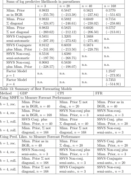
The list of 168 variables used in this study, running from 1959Q1 through 2008Q4, is given in the Data Appendix. Following Stock and Watson (2008) and many others, the variables are all transformed to stationarity (usually by di¤erencing or log di¤erencing) as described in the Data Appendix. All data are then standardized by subtracting o¤ the mean and dividing by the standard deviation. Note that this means that our prior means for all coe¢ cients in all approaches are set to zero (instead of setting some prior means to one so as to shrink towards a random walk as would be appropriate if we were working with untransformed variables).

The variables are divided into four groups. The variables in BGR’s data set are not identical to those in ours, so we do not match their setup exactly, but the following choices are similar to and motivated by their grouping of variables. The …rst group contains the three main variables we are interested in forecasting. These are a measure of economic activity (GDP, real GDP), prices (CPI, the consumer price index) and an interest rate (FFR, the Fed funds rate).3 _{The second group contains an additional}

17 variables which, added to the three main variables leads to the n = 20 variables used by BGR in their medium VAR. The choice of these variables is partly motivated the monetary model of Christiano, Eichenbaum and Evans (1999) and partly includes variables found to be useful for forecasting in other studies. The third group contains an additional 20 variables (combined with the other groups, this leads to a larger VAR with n = 40 variables). These 20 variables have sometimes been found to be useful in forecasting exercises. This group contains most of the remaining aggregate variables in the data set. The remainder of the 168 variables are in a …nal group. These are mostly the components making up the aggregate variables already included in the other groups. We thus have small VARs (with n = 3), medium VARs (n = 20), medium-large VARs (n= 40) and large VARs (n = 168). Note that BGR found most of the gains in forecast performance through the use of more variables to have been achieved by using medium VARs, with large VARs forecasting approximately as well as medium VARs. All approaches use four lags of the dependent variables (p= 4).

3.2 Forecast Metrics

Our rolling and recursive forecast exercises provide us with the predictive density for

y +h using data available through time for h = 1 and 4. For the rolling forecasts,

we use a window of ten years. The predictive density is evaluated for = 0; ::; T h

where 0 is 1969Q4. We use notation where y +h is a random variable we are wishing

to forecast (e.g. GDP, CPI or FFR), yo

+h is the observed value of the random variable

y +handp(y +hjData )is the predictive density based on information available at time

.

The most common measure of forecast performance is MSFE where:

3_{The transformations used on the data means we are forecasting the di¤erence of log GDP, the}

(12)

M SF E=

PT h

= 0 y

o

+h E(y +hjData )

2

T h 0+ 1

:

However, this only uses the point forecasts and ignores the rest of the predictive dis-tribution. For this reason, we also use the predictive likelihood to evaluate forecast performance. Note that a great advantage of predictive likelihoods is that they evalu-ate the forecasting performance of the entire predictive density. Predictive likelihoods are motivated and described in many places such as Geweke and Amisano (2009). The predictive likelihood is the predictive density for y +h evaluated at the actual outcome

yo

+h. We use the sum of log predictive likelihoods for forecast evaluation: T h

X

= 0

log p y +h =yo+hjData :

3.3 Forecasting Approaches

To the three general categories of forecasting methods for Bayesian VARs described above (i.e. Minnesota prior, Non-conjugate SSVS and Conjugate SSVS) we add the category of traditional factor models as a benchmark for comparison. Within each category we have various ways implementations as described in this sub-section.

3.3.1 Minnesota Priors

We consider three variants of the Minnesota prior: the …rst is as in BGR (labelled “Minn. Prior as in BGR”in the tables below). The second is the traditional Minnesota prior (labelled “Minn. Prior diagonal”). The third is the traditional Minnesota prior except that the upper left 3 3 block of is not assumed to be diagonal (labelled “Minn. Prior not diagonal”). Details of how these are implemented were given in Section 2.1

The Minnesota prior of BGR requires the selection of a single shrinkage parameter, . We choose this in the same manner as BGR. To be precise, an initial set of data is set aside as a training sample (we use all data through 1969Q4 for this purpose). Using this entire training sample we estimate the VARs and then use them for forecasting within this training sample. In medium, medium-large and large VARs, is chosen so as to yield a …t in this training sample as close as possible to the small VAR for the three main variables being forecast. For the small VAR no shrinkage is done ( _{! 1}).

Fit is de…ned as:

F it n=

1 3

3

X

i=1

M SF E(i; ; n)

M SF E(i;0;3)

whereM SF E(i; ; n)is the MSFE of variableiusing shrinkage parameter in a VAR with n variables. Note that M SF E(i;0;3)is simply the MSFE produced by the prior in the small VAR which is used to normalize the measure. For the VAR withnvariables we choose to minimize:

(13)

Grid search methods are used to solve this minimization problem.

For the other two variants of the Minnesota prior we adopt a similar strategy of matching …t with a small VAR in a training sampler. However, here we have two shrinkage parameters ( 1 which controls shrinkage of coe¢ cients on own lags and 2

which controls shrinkage of coe¢ cients on other lags) and do a two-dimensional grid search to minimize the di¤erence in …t between the VAR withnvariables and the small VAR with no shrinkage.

3.3.2 The SSVS Priors

We implement the non-conjugate SSVS prior approach in two ways. First, we use the “default semi-automatic approach” to prior elicitation suggested by George, Sun and Ni (2008). This involves setting 0j = c0

p d

var( j) and 1j = c1

p d

var( j) where d

var( j) is an estimate of the variance of the coe¢ cient in an unrestricted VAR. In

our case, _dvar( j) is the posterior variance of j obtained from the corresponding VAR

using BGR’s prior. The pre-selected constants c0 and c1 must have c0 c1 and we set

c0 = 0:1 and c1 = 10. Note that this means the semi-automatic prior is a data-based

prior. This is labelled “SSVS Non-conj. semi-automatic” in the tables below.

An alternative would be to use the approach just described but choose _dvar( j) in

a manner which did not involve the data. A natural choice suggests itself: set _dvar( j)

to be the prior variance from BGR’s Minnesota prior. We do this, settingc0 = 0:1 and

c1 = 1. The results is a prior which has the attractive property that it combines the

Minnesota prior with the SSVS prior. That is, if _j = 1 for j = 1; ::; K, we obtain a prior which is identical to the one used by BGR. But if j = 0 for some j, then this

prior allows for additional shrinkage beyond that used in the Minnesota prior. And it decides in a data-based fashion whether this extra shrinkage is warranted or not. This is labelled “SSVS Non-conj. plus Minn. Prior” in the tables below.

For the conjugate SSVS prior we use the same two approaches: one a semi-default automatic approach and one which combines the SSVS prior with the Minnesota prior. All details are as above with one exception. Remember that the conjugate SSVS prior either includes or excludes each variable in every equation (rather than includ-ing/excluding individual coe¢ cients like the non-conjugate SSVS prior). Hence, we set the _dvar( j) term to be the maximum value for this variance which occurs in any

equation. Results for these priors are labelled “SSVS Conjugate semi-automatic” and “SSVS Conjugate plus Minn. Prior” in the tables below.

For the reasons discussed in Section 2.2, it is computationally infeasible to use the non-conjugate SSVS priors with large or even medium-large VARs and, accordingly, we only present results for VARs with n = 3 and 20. With the conjugate SSVS priors, we present results for VARs withn= 3;20and40, but …ndn = 168to be computationally infeasible and do not present results for the latter case.

3.3.3 Factor Methods

(14)

and four lags of these factors, respectively. These are labelled “Factor Model p = 1” and “Factor Modelp= 4”, respectively, in the tables below.

3.4 Results

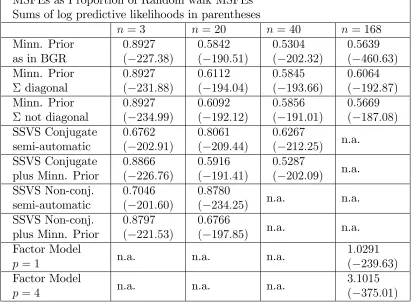
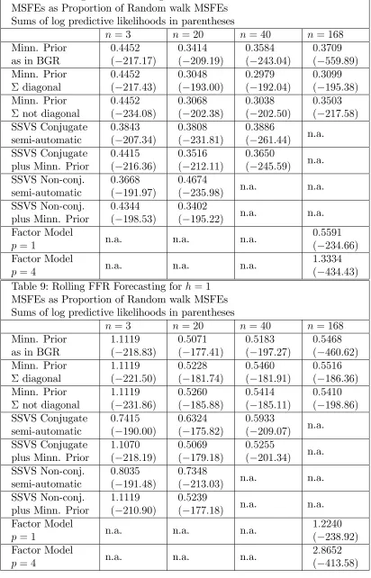
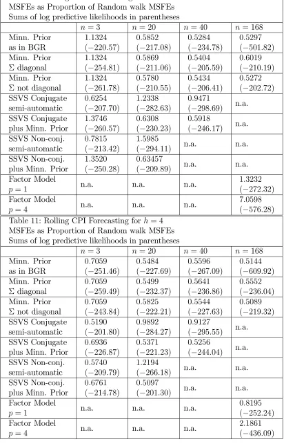
Tables 1 through 12 present the results for all our forecasting exercises. The 12 tables arise from our forecasting three variables at two forecasting horizons using recursive and rolling methods. Table 13 provides a summary, listing the single approach which performs best for each of these 12 cases. The upper half of Table 13 uses MSFEs to decide what is “best” while the lower half uses sums of log predictive likelihoods.

There is no one single strong story arising from our empirical results saying, e.g., that one single forecasting method predominates. Our di¤erent approaches balance the tension between including more information and ensuring more/di¤erent shrinkage in di¤erent ways. We cannot say theoretically that one way is better than another, what works will is an empirical matter. In practice we …nd some approaches doing well in some cases, but not necessarily in others. Nevertheless, a few interesting stories emerge. Note …rst that factor methods never lead to the best forecast performance. In all cases, most of our ways of implementing VARs lead to better (and often much better) forecast performance. This con…rms the …ndings made by BGR using a di¤erent data set. At a minimum, we have established that working with high-dimensional Bayesian VARs is an alternative worth considering when working with large panels of data.

The results indicate, though, that there is no single approach to VAR forecasting that is predominant. If we take our 12 cases and note that forecast performance can either be evaluated using MSFEs or sums of log predictive likelihoods, we have 24 forecasting “races”. In these races, SSVS approaches have 13 “wins” and Minnesota prior approaches win 11 times, a very even split. In terms of VAR dimensionality, large, medium-large and medium VARs each win …ve times and small VARs win nine times, also a fairly even split. In short, virtually every one of our VAR approaches does well for some variable, forecast horizon or forecasting metric.

Despite the fact that small VARs often forecast well, often we do …nd that moving away from small VARs does lead to improved forecast performance. That is, reading across any row in Tables 1 through 12 we typically …nd that the MSFEs or sums of log predictive likelihoods decrease. However, it is worth noting that in most cases, these decreases are small or non-existent when we move beyond n = 20. This also is consistent with BGRs …nding that most of the gains found in VAR forecasting are obtained by using 20 variables and that adding more variables beyond this often yields only slight improvements (or even deterioration) in forecast performance.

However, there are many exceptions to the pattern noted in the preceding paragraph. These exceptions almost invariably occur with the SSVS priors and h = 4. With the Minnesota priors it is virtually always the case that moving from n = 3 to n = 20

(15)

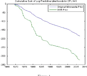
When we compare the various implementations of Minnesota priors, we …nd that BGR’s speci…cation often works well. However, in terms of MSFEs, it is often the case that one of the alternative implementations forecasts slightly better. These alternatives are characterized by di¤erent degrees of shrinkage for the coe¢ cients on own lags than on other lags, and it does seem that this often improves forecast performance. Our version of the original Minnesota prior which allows for the upper left 3 3block of to be unrestricted often forecasts quite well. In terms of MSFEs, it appears that the advantages of having a completely unrestricted (as in BGR) are relatively small. In terms of sums of log predictive likelihoods, it appears that allowing for an unrestricted can occasionally lead to very poor forecast performance. As an example, consider recursively forecasting CPI forh= 1. In terms of MSFEs, the best forecasting method uses a variant of the original Minnesota prior with a 20-variate VAR. The MSFE is

0:2664. If we consider large VARs with n = 168, the MSFEs are only slightly higher (0:2834 for the original Minnesota prior and 0:3309 for BGR’s prior). However, with these large VARs the sum of log predictive likelihoods is vastly di¤erent between the original Minnesota prior ( 184:78) and BGR’s prior ( 322:27). To shed more light on this case, Figures 1 and 2 plots the cumulative sum of log predictive likelihoods and cumulative sum of squared forecast errors, respectively, for these two priors. The cumulative sum of squared forecast errors for these two approaches track each other fairly closely, with the exception of the early 1980s. However, the cumulative sum of log predictive likelihoods are much more di¤erent, with the two lines diverging substantially in the period 1975-1985 and again at the end of the sample. This shows that the point forecasts of these two approaches are similar to one another. However, other features of the predictive density are quite di¤erent. In this case, what is happening is that BGR’s approach tends to yield an unnecessarily disperse predictive distribution due to its need to estimate so many more parameters (i.e. in the BGR approach contains

n(n+1)

2 parameters to be estimated, whereas the original Minnesota prior only has n

parameters in and these are replaced by simple estimates). Even if the mean of the predictive density provides a good point forecast, an unnecessarily large predictive standard deviation mean that the predictive likelihood evaluated at the outcome will be lower than a predictive without such a large standard deviation. When looking at large VARs (particularly using BGR’s prior), we often …nd this pattern of good MSFEs but poor sums of log predictive likelihoods. A related …nding is that small VARs tend to forecast particularly well when we use sums of log predictive likelihoods to evaluate forecast performance, but there is less evidence of this when using MSFEs. By focussing solely on MSFEs, the researcher would miss important empirical …ndings such as these. When we compare various implementations of the SSVS priors, few strong patterns emerge. The non-conjugate SSVS prior often forecasts slightly better than the conju-gate variant. Using the Minnesota prior to calibrate the prior for the SSVS approach often improves forecast performance. But there are many exceptions to both of these statements.

(16)

Table 1: GDP Forecasting for h= 1

MSFEs as Proportion of Random walk MSFEs Sums of log predictive likelihoods in parentheses

n= 3 n= 20 n = 40 n = 168

Minn. Prior as in BGR

0:6504 ( 206:37)

0:5552 ( 192:29)

0:5084 ( 186:60)

0:5225 ( 223:78)

Minn. Prior diagonal

0:7065 ( 211:85)

0:5774 ( 204:84)

0:6381 ( 205:52)

0:5631 ( 202:39)

Minn. Prior not diagonal

0:7065 ( 205:97)

0:5489 ( 195:40)

0:5402 ( 193:49)

0:5305 ( 192:81)

SSVS Conjugate semi-automatic

0:6338 ( 200:66)

0:6776 ( 199:90)

0:6983

( 197:66) n.a.

SSVS Conjugate plus Minn. Prior

0:6062 ( 198:77)

0:5577 ( 192:53)

0:5368

( 192:44) n.a.

SSVS Non-conj. semi-automatic

0:6061 ( 198:40)

0:6407

( 205:12) n.a. n.a.

SSVS Non-conj. plus Minn. Prior

0:6975 ( 204:71)

0:6466

( 203:92) n.a. n.a.

Factor Model

p= 1 n.a. n.a. n.a.

0:6441 ( 195:10)

Factor Model

p= 4 n.a. n.a. n.a.

0:7657 ( 207:67)

Table 2: CPI Forecasting for h= 1

n= 3 n= 20 n = 40 n = 168

0:3471 ( 201:23)

0:3029 ( 195:90)

0:3172 ( 210:09)

0:3309 ( 322:27)

0:3317 ( 190:85)

0:2756 ( 182:18)

0:3252 ( 200:55)

0:2834 ( 184:78)

0:3317 ( 203:95)

0:2664 ( 184:06)

0:2718 ( 188:27)

0:3019 ( 197:45)

0:3138 ( 187:82)

0:2724 ( 191:15)

0:3061

( 197:66) n.a.

0:3086 ( 186:70)

0:3088 ( 197:64)

0:3601

( 222:30) n.a.

0:3197 ( 193:92)

0:3161

( 196:47) n.a. n.a.

0:3252 ( 191:45)

0:2910

( 187:58) n.a. n.a.

Factor Model

p= 1 n.a. n.a. n.a.

0:3133 ( 191:83)

Factor Model

p= 4 n.a. n.a. n.a.

(17)

Table 3: FFR Forecasting for h= 1

n= 3 n= 20 n = 40 n = 168

0:6192 ( 238:40)

0:5136 ( 229:14)

0:5084 ( 243:71)

0:5224 ( 266:66)

0:8351 ( 247:02)

0:5355 ( 238:79)

0:6218 ( 263:05)

0:5532 ( 239:84)

0:8351 ( 267:29)

0:5164 ( 249:09)

0:5530 ( 249:49)

0:5223 ( 258:28)

0:7944 ( 247:25)

0:6329 ( 245:25)

0:5936

( 256:02) n.a.

0:7554 ( 243:16)

0:5134 ( 228:54)

0:5354

( 251:98) n.a.

0:8439 ( 252:43)

0:5790

( 237:16) n.a. n.a.

0:7436 ( 252:68)

0:5431

( 228:86) n.a. n.a.

Factor Model

p= 1 n.a. n.a. n.a.

0:7360 ( 232:66)

Factor Model

p= 4 n.a. n.a. n.a.

0:7466 ( 237:99)

Table 4: GDP Forecasting for h= 4

n= 3 n= 20 n = 40 n = 168

0:7437 ( 220:57)

0:6094 ( 214:71)

0:5717 ( 214:38)

0:5420 ( 277:46)

0:7437 ( 219:25)

0:6100 ( 214:02)

0:5728 ( 210:99)

0:5656 ( 210:06)

0:7437 ( 220:58)

0:6214 ( 213:28)

0:5831 ( 209:50)

0:5780 ( 209:37)

0:6129 ( 211:36)

0:6473 ( 212:35)

0:8881

( 239:87) n.a.

0:8404 ( 222:91)

0:8357 ( 219:64)

0:6387

( 222:50) n.a.

0:6147 ( 207:80)

0:7535

( 293:21) n.a. n.a.

0:8438 ( 221:57)

0:6670

( 219:01) n.a. n.a.

Factor Model

p= 1 n.a. n.a. n.a.

0:7662 ( 223:24)

Factor Model

p= 4 n.a. n.a. n.a.

(18)

Table 5: CPI Forecasting for h= 4

n= 3 n= 20 n = 40 n = 168

0:5254 ( 209:51)

0:5217 ( 219:35)

0:5246 ( 235:65)

0:5044 ( 262:55)

0:5254 ( 216:43)

0:5191 ( 217:60)

0:5207 ( 218:45)

0:5124 ( 216:64)

0:5254 ( 214:64)

0:5203 ( 216:07)

0:5214 ( 217:57)

0:5197 ( 217:14)

0:4990 ( 211:36)

0:6042 ( 225:02)

0:6847

( 253:84) n.a.

0:4759 ( 199:86)

0:7031 ( 246:64)

0:4853

( 220:44) n.a.

0:5010 ( 208:26)

0:7723

( 226:36) n.a. n.a.

0:4683 ( 194:39)

0:4883

( 201:62) n.a. n.a.

Factor Model

p= 1 n.a. n.a. n.a.

0:5608 ( 214:72)

Factor Model

p= 4 n.a. n.a. n.a.

0:6258 ( 228:84)

Table 6: FFR Forecasting for h= 4

n= 3 n= 20 n = 40 n = 168

0:6679 ( 243:31)

0:5868 ( 249:63)

0:5670 ( 264:80)

0:5717 ( 319:40)

0:6679 ( 281:95)

0:6075 ( 278:11)

0:5946 ( 273:70)

0:6379 ( 281:92)

0:6679 ( 246:90)

0:5882 ( 244:77)

0:5894 ( 240:50)

0:6362 ( 245:34)

0:5508 ( 236:00)

0:5873 ( 249:46)

0:7408

( 273:60) n.a.

0:6259 ( 235:57)

0:6716 ( 258:47)

0:5370

( 255:89) n.a.

0:5265 ( 231:16)

0:8811

( 268:06) n.a. n.a.

0:6184 ( 228:80)

0:5282

( 233:67) n.a. n.a.

Factor Model

p= 1 n.a. n.a. n.a.

0:7027 ( 244:52)

Factor Model

p= 4 n.a. n.a. n.a.

(19)

[image:19.612.129.542.78.380.2]

Table 7: Rolling GDP Forecasting for h= 1

n= 3 n= 20 n = 40 n = 168

0:8927 ( 227:38)

0:5842 ( 190:51)

0:5304 ( 202:32)

0:5639 ( 460:63)

0:8927 ( 231:88)

0:6112 ( 194:04)

0:5845 ( 193:66)

0:6064 ( 192:87)

0:8927 ( 234:99)

0:6092 ( 192:12)

0:5856 ( 191:01)

0:5669 ( 187:08)

0:6762 ( 202:91)

0:8061 ( 209:44)

0:6267

( 212:25) n.a.

0:8866 ( 226:76)

0:5916 ( 191:41)

0:5287

( 202:09) n.a.

0:7046 ( 201:60)

0:8780

( 234:25) n.a. n.a.

0:8797 ( 221:53)

0:6766

( 197:85) n.a. n.a.

Factor Model

p= 1 n.a. n.a. n.a.

1:0291 ( 239:63)

Factor Model

p= 4 n.a. n.a. n.a.

(20)

[image:20.612.129.541.69.711.2]

Table 8: Rolling CPI Forecasting for h= 1

n= 3 n= 20 n = 40 n = 168

0:4452 ( 217:17)

0:3414 ( 209:19)

0:3584 ( 243:04)

0:3709 ( 559:89)

0:4452 ( 217:43)

0:3048 ( 193:00)

0:2979 ( 192:04)

0:3099 ( 195:38)

0:4452 ( 234:08)

0:3068 ( 202:38)

0:3038 ( 202:50)

0:3503 ( 217:58)

0:3843 ( 207:34)

0:3808 ( 231:81)

0:3886

( 261:44) n.a.

0:4415 ( 216:36)

0:3516 ( 212:11)

0:3650

( 245:59) n.a.

0:3668 ( 191:97)

0:4674

( 235:98) n.a. n.a.

0:4344 ( 198:53)

0:3402

( 195:22) n.a. n.a.

Factor Model

p= 1 n.a. n.a. n.a.

0:5591 ( 234:66)

Factor Model

p= 4 n.a. n.a. n.a.

1:3334 ( 434:43)

Table 9: Rolling FFR Forecasting for h= 1

n= 3 n= 20 n = 40 n = 168

1:1119 ( 218:83)

0:5071 ( 177:41)

0:5183 ( 197:27)

0:5468 ( 460:62)

1:1119 ( 221:50)

0:5228 ( 181:74)

0:5460 ( 181:91)

0:5516 ( 186:36)

1:1119 ( 231:86)

0:5260 ( 185:88)

0:5414 ( 185:11)

0:5410 ( 198:86)

0:7415 ( 190:00)

0:6324 ( 175:82)

0:5933

( 209:07) n.a.

1:1070 ( 218:19)

0:5069 ( 179:18)

0:5255

( 201:34) n.a.

0:8035 ( 191:48)

0:7348

( 213:03) n.a. n.a.

1:1119 ( 210:90)

0:5239

( 177:18) n.a. n.a.

Factor Model

p= 1 n.a. n.a. n.a.

1:2240 ( 238:92)

Factor Model

p= 4 n.a. n.a. n.a.

(21)

[image:21.612.129.541.68.713.2]

Table 10: Rolling GDP Forecasting for h= 4

n= 3 n= 20 n = 40 n = 168

1:1324 ( 220:57)

0:5852 ( 217:08)

0:5284 ( 234:78)

0:5297 ( 501:82)

1:1324 ( 254:81)

0:5869 ( 211:06)

0:5404 ( 205:59)

0:6019 ( 210:19)

1:1324 ( 261:78)

0:5780 ( 210:55)

0:5434 ( 206:41)

0:5272 ( 202:72)

0:6254 ( 207:70)

1:2338 ( 282:63)

0:9471

( 298:69) n.a.

1:3746 ( 260:57)

0:6308 ( 230:23)

0:5918

( 246:17) n.a.

0:7815 ( 213:42)

1:5985

( 294:11) n.a. n.a.

1:3520 ( 250:28)

0:63457

( 209:89) n.a. n.a.

Factor Model

p= 1 n.a. n.a. n.a.

1:3232 ( 272:32)

Factor Model

p= 4 n.a. n.a. n.a.

7:0598 ( 576:28)

Table 11: Rolling CPI Forecasting for h= 4

n= 3 n= 20 n = 40 n = 168

0:7059 ( 251:46)

0:5484 ( 227:69)

0:5596 ( 267:09)

0:5144 ( 609:92)

0:7059 ( 259:49)

0:5499 ( 232:37)

0:5641 ( 236:86)

0:5552 ( 236:04)

0:7059 ( 243:84)

0:5825 ( 222:21)

0:5544 ( 227:63)

0:5089 ( 219:32)

0:5190 ( 201:80)

0:9892 ( 284:27)

0:9127

( 295:55) n.a.

0:6936 ( 226:87)

0:5371 ( 221:23)

0:5256

( 244:04) n.a.

0:5740 ( 209:79)

1:2194

( 266:18) n.a. n.a.

0:6761 ( 214:78)

0:5097

( 201:30) n.a. n.a.

Factor Model

p= 1 n.a. n.a. n.a.

0:8195 ( 252:24)

Factor Model

p= 4 n.a. n.a. n.a.

(22)

Table 12: Rolling FFR Forecasting for h= 4

n= 3 n= 20 n = 40 n = 168

0:9833 ( 255:70)

0:5847 ( 213:38)

0:5621 ( 237:84)

0:5770 ( 551:63)

0:9833 ( 324:87)

0:5882 ( 246:61)

0:6049 ( 238:02)

0:7154 ( 258:66)

0:9833 ( 269:62)

0:5825 ( 212:12)

0:6026 ( 206:50)

0:5757 ( 213:01)

0:5851 ( 207:19)

1:3205 ( 273:83)

1:1668

( 275:46) n.a.

0:9152 ( 241:89)

0:6059 ( 213:50)

0:5674

( 228:79) n.a.

0:5516 ( 197:78)

1:6380

( 268:75) n.a. n.a.

0:9083 ( 228:57)

0:5830

( 198:07) n.a. n.a.

Factor Model

p= 1 n.a. n.a. n.a.

1:2547 ( 273:95)

Factor Model

p= 4 n.a. n.a. n.a.

[image:22.612.120.561.87.678.2]

3:7353 ( 514:91)

Table 13: Summary of Best Forecasting Models

Method GDP CPI FFR

Using MSFE to Measure Forecast Performance

h= 1, rec. Minn. Prior

as in BGR, n = 40

Minn. Prior not diag., n= 20

Minn. Prior as in BGR,n = 40

h= 4, rec. Minn. Prior

as in BGR, n = 168

SSVS Non-conj plus Minn. Prior, n = 3

SSVS Non-conj. semi-auto.,n = 3

h= 1, roll. SSVS Conj. plus Minn. Prior, n= 40

Minn. Prior

diagonal, n= 40

SSVS Conj. plus Minn. Prior, n= 20

h= 4, roll. Minn. Prior, not diagonal, n= 168

Minn. Prior not diagonal, n = 168

SSVS Non-conj. semi-auto.,n = 3

Using Pred. Likes. to Measure Forecast Performance

h= 1, rec. Minn. Prior as in BGR, n = 40

Minn. Prior diag.,n = 20

SSVS Conj. plus Minn. Prior, n= 20

h= 4, rec. SSVS Non-conj. semi-auto., n = 3

SSVS Non-conj plus Minn. Prior, n = 3

SSVS Non-conj plus Minn. Prior, n= 3

h= 1, roll. Minn. Prior not diagonal, n= 168

SSVS Non-conj. semi-auto., n= 3

SSVS Conjugate semi-auto.,n = 20

h= 4, roll. Minn. Prior not diagonal, n= 168

SSVS Conjugate semi-auto., n= 3

(23)

[image:23.612.186.479.77.335.2]

Figure 1

Figure 2

4 Conclusions

(24)

medium and large VARs. These issues are both computational and theoretical. The computational issues arise since priors which are not conjugate (or are only conditionally conjugate) typically require the use of posterior simulation methods. Non-conjugate priors typically have properties which are, in theory, more attractive. However, the researcher runs into computational problems which can be substantial (in the case of VARs with 20-40 dependent variables) or prohibitive (in the case of VARs with 50 or more dependent variables). The theoretical issues arise since the various priors shrink forecasts to di¤erent degrees and in di¤erent ways. A careful balancing of these computational and theoretical concerns is crucial to any sensible empirical analysis. This paper provides theoretical and empirical evidence relating to how this balancing might be done.

In particular, this paper presents several priors which have the potential for being useful for VAR forecasting. We focus on the classes of Minnesota and SSVS priors. The properties of these priors are discussed with emphasis on the issues which arise when moving from small to medium to large VARs. Our empirical exercise suggests that Bayesian VARs do tend to forecast better than factor methods. But there is no single prior which consistently leads to the best forecasting performance.

(25)

References

Banbura, M., Giannone, D. and Reichlin, L. (2010). “Large Bayesian Vector Auto Regressions,”Journal of Applied Econometrics, 25, 71-92.

Brown, P., Vannucci, M. and Fearn, T. (1998). “Multivariate Bayesian variable selection and prediction,”Journal of the Royal Statistical Society B, 60, 627-641.

Christiano, L., Eichenbaum, M. and Evans C. (1999). “Monetary policy shocks: what have we learned and to what end?”Handbook of Macroeconomics, Vol. 1, ch. 2, p. 65-148, Taylor J., Woodford M. (eds). Elsevier: Amsterdam.

Doan, T., Litterman, R. and Sims, C. (1984). “Forecasting and conditional projec-tion using realistic prior distribuprojec-tions,”Econometric Reviews, 3, 1-144.

Forni, M., Hallin, M., Lippi, M. and Reichlin, L. (2003). “Do …nancial variables help forecasting in‡ation and real activity in the Euro Area?”Journal of Monetary

Economics, 50, 1243–1255.

George, E., Sun, D. and Ni, S. (2008). “Bayesian stochastic search for VAR model restrictions,”Journal of Econometrics, 142, 553-580.

Geweke, J. and Amisano, J. (2009). “Hierarchical Markov normal mixture models with applications to …nancial asset returns,”Journal of Applied Econometrics, forth-coming.

Jochmann, M., Koop, G. and Strachan, R. (2009). “Bayesian forecasting using stochastic search variable selection in a VAR subject to breaks,”International Journal of Forecasting, forthcoming.

Kadiyala, K. and Karlsson, S. (1997). “Numerical methods for estimation and inference in Bayesian VAR models,”Journal of Applied Econometrics, 12, 99-132.

Koop, G. and Potter, S. (2004). “Forecasting in dynamic factor models using Bayesian model averaging,”The Econometrics Journal, 7, 550-565.

Korobilis, D. (2009). “Forecasting in Vector Autoregressions with many predictors,”

Advances in Econometrics, vol. 23: Bayesian Macroeconometrics, forthcoming.

Litterman, R. (1986). “Forecasting with Bayesian vector autoregressions – Five years of experience,”Journal of Business and Economic Statistics, 4, 25-38.

Marcellino, M., Stock, J. and Watson, M. (2006). “A comparison of direct and iterated multistep AR methods for forecasting macroeconomic time series,”Journal of Econometrics, 135, 499–526.

Poirier, D. (1998). “Revising beliefs in non-identi…ed models,”Econometric Theory, 14, 483-509.

Stock, J. and Watson, M. (2002). “Macroeconomic forecasting using di¤usion in-dexes,”Journal of Business and Economic Statistics, 20, 147-162.

Stock, J. and Watson, M. (2006). “Forecasting using many predictors,”pp. 515-554

in Handbook of Economic Forecasting, Volume 1, edited by G. Elliott, C. Granger and

A. Timmerman, Amsterdam: North Holland.

Stock, J. and Watson, M. (2008). “Forecasting in dynamic factor models subject to structural instability,”inThe Methodology and Practice of Econometrics, A Festschrift

in Honour of Professor David F. Hendry, edited by J. Castle and N. Shephard, Oxford:

(26)

Appendix A: Technical Details

MCMC Algorithm for the VAR with Non-conjugate SSVS Prior

Posterior computation in the VAR with SSVS prior can be carried out using the MCMC algorithm described in George, Sun and Ni (2008). We use notation where denotes all the parameters in the VAR with non-conjugate SSVS prior and ( a)denotes

all the parameters except for a. For the notation used in this appendix, please refer to Section 2.2.

For the VAR coe¢ cients we have

jY; ( ) N( ; V ); (16)

where

V = [ 1 (X0X) +D 1] 1;

=V D 1 +vec(X0Y 1) :

The conditional posterior for has jbeing independent (for allj) Bernoulli random

variables:

Pr

h

j = 1jY; ₍ _j₎ i

=q_j;

Prh _j = 0_jY; ₍

j)

i

= 1 q_j;

(17)

where

q_j =

1

1j

exp

2

j

2 2 1j

q

j

1

1j

exp

2

j

2 2 1j

q

j +

1

0j

exp

2

j

2 2 0j

1 q

j

:

For the error covariance matrix, we begin with the following decomposition:

1 ₌ 0_; ₍₁₈₎

where is upper-triangular. We use a Gamma prior for the square of each of the diagonal elements of and the SSVS mixture of normals prior for each element above the diagonal. Note that this implies that the diagonal elements of are always included in the model, ensuring a positive de…nite error covariance matrix.

Let the non-zero elements of be labelled as ij and de…ne = ( 11; ::; nn)0,

j = ( 1j; ::; j 1;j)0 forj = 2; ::; nand = ( 02; ::; 0n)0. For the diagonal elements of ,

we assume prior independence from each other and:

2

jj G aj; bj ; (19)

(27)

The hierarchical prior for the o¤-diagonal elements of takes the same mixture of normals form as . In particular, the SSVS prior has

jj!j N(0; Fj); (20)

where !j = (!1j; ::; !j 1;j)0 is a vector of unknown parameters with typical element

!ij 2 f0;1g, and Fj =diag(f1j; ::; fj 1;j) where

fij =

2

0ij if !ij = 0

2

1ij if !ij = 1

; (21)

for j = 2; ::; n and i = 1; ::; j 1. Reasonable small and large prior hyperparameter

values are 0ij = 0:1 and 1ij = 1:0.

For ! = (!0

2; ::; !0n)0, the SSVS prior posits that each element has a Bernoulli form

(independent of the other elements of !) and, hence, we have

Pr (!ij = 1) =q_ij,

Pr (!ij = 0) = 1 q_ij. (22)

We make the default choice of q

ij = 0:5 for all j and i so that, a priori, each

parameter is equally likely to be included or excluded.

The conditional posterior for can be obtained by noting that the conditional posterior for 2_jj (for j = 1; : : : ; n) are independent of one another with

2

jjjY; ₍ _jj₎ G aj+

T

2; bj ; (23)

where

bj =

(

b1 +v11₂ , if j = 1,

b1 +1₂

n

vjj vj0 Vj 1+ (Fj)

1 1

vj o

, if j = 2; : : : ; n:

The preceding equation uses notation where

V = (Y XA)0(Y XA)

has elements vij,vj = (v1j; : : : ; vj 1;j)0 and Vj is the upper left j j block ofV.

The conditional posterior of can be written in terms of the conditional posteriors

of j (forj = 2; : : : ; n) being independent of one another with:

jjY; ₍ _j₎ N j; Vj ; (24)

where

Vj = Vj 1+Fj 1

and

j = jjVjvj:

Finally, the conditional posterior for!has!ij being independent (for allij) Bernoulli

(28)

Pr !ij = 1jY; ( !ij) =qij; Pr !ij = 0jY; ( !ij) = 1 qij;

(25)

where

q_ij =

1

1ij

exp

2

ij

2 2 1ij

!

q

ij

1

1ij

exp

2

ij

2 2 1ij

!

q

ij +

1

0ij

exp

2

ij

2 2 0ij

!

1 q

ij

:

In summary, an MCMC algorithm for the VAR with non-conjugate SSVS prior involves sequentially drawing from (16), (17), (23), (24) and (25).

Posterior Simulation Algorithm for the VAR with Conjugate SSVS

Prior

The formula for posterior and predictive densities for the VAR with natural con-jugate prior are given in Section 2.1 of the paper. For the VAR with concon-jugate SSVS prior, they can be interpreted as holding, conditional on_e. Thus, all that is required is

p(_e_jY). Using standard formula for the marginal likelihood for the multivariate Normal regression model and a noninformative prior for_e we obtain:

p(_e_jY)_{/ j}D _j V 1

n

2

S

T+n+ 1 2

(29)

Appendix B: Data

[image:29.612.114.574.230.591.2]

The data set used in this paper is an updated version of that used in Stock and Watson (2008) and the reader is referred to that paper for more details about the data. The raw data runs from 1959Q1 through 2008Q4. Variables which are originally at a monthly frequency are transformed to a quarterly by averaging over the three months in a quarter. Except for …nancial variables, variables are seasonally adjusted. All variables are transformed to stationarity as in Stock and Watson (2008). The following table provides a brief description of each variable along with a transformation code. This code is: 1 = no transformation, 2 = …rst di¤erence, 3 = second di¤erence, 4 = log, 5 = …rst di¤erence of logged variables, 6 = second di¤erence of logged variables.

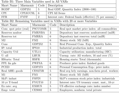
Table B1: Three Main Variables used in All VARs Short Name Mnemonic Code Description

RGDP GDP251 5 Real GDP, Quantity Index (2000=100) CPI CPIAUCSL 6 CPI All Items

FFR FYFF 2 Interest rate: Federal funds (e¤ective) (% per annum)

Table B2: Remaining Variables used in VARs with 20 or more Variables Short Name Mnemonic Code Description

Com: spot price (real) PSCCOMR 5 Real spot market price index: all commodities Reserves nonbor FMRNBA 3 Depository inst reserves: nonborrowed (mil$) Reserves tot FMRRA 6 Depository inst reserves: total (mil$)

M2 FM2 6 Money stock: M2 (bil$)

Cons GDP252 5 Real Personal Cons. Exp., Quantity Index IP: total IPS10 5 Industrial production index: total

Capacity Util UTL11 1 Capacity utilization: manufacturing (SIC) U: all LHUR 2 Unemp. rate: All workers, 16 and over (%) HStarts: Total HSFR 4 Housing starts: Total (thousands)

PPI: …n gds PWFSA 6 Producer price index: …nished goods PCED GDP273 6 Personal Consumption Exp.: price index

Real AHE: goods CES275R 5 Real avg hrly earnings, non-farm prod. workers M1 FM1 6 Money stock: M1 (bil$)

(30)

[image:30.612.113.578.62.384.2]

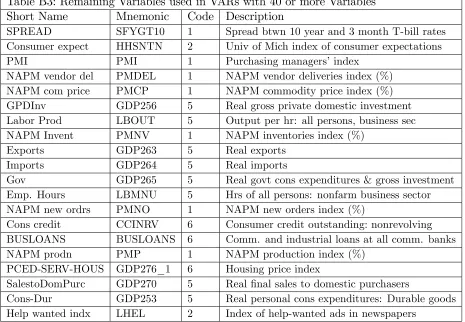
Table B3: Remaining Variables used in VARs with 40 or more Variables Short Name Mnemonic Code Description

SPREAD SFYGT10 1 Spread btwn 10 year and 3 month T-bill rates Consumer expect HHSNTN 2 Univ of Mich index of consumer expectations PMI PMI 1 Purchasing managers’index

NAPM vendor del PMDEL 1 NAPM vendor deliveries index (%) NAPM com price PMCP 1 NAPM commodity price index (%) GPDInv GDP256 5 Real gross private domestic investment Labor Prod LBOUT 5 Output per hr: all persons, business sec NAPM Invent PMNV 1 NAPM inventories index (%)

Exports GDP263 5 Real exports Imports GDP264 5 Real imports

Gov GDP265 5 Real govt cons expenditures & gross investment Emp. Hours LBMNU 5 Hrs of all persons: nonfarm business sector NAPM new ordrs PMNO 1 NAPM new orders index (%)

Cons credit CCINRV 6 Consumer credit outstanding: nonrevolving BUSLOANS BUSLOANS 6 Comm. and industrial loans at all comm. banks NAPM prodn PMP 1 NAPM production index (%)

PCED-SERV-HOUS GDP276_1 6 Housing price index

SalestoDomPurc GDP270 5 Real …nal sales to domestic purchasers

(31)

[image:31.612.113.577.59.508.2]

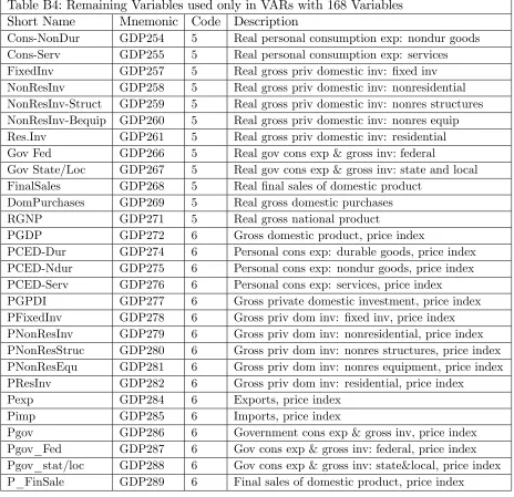
Table B4: Remaining Variables used only in VARs with 168 Variables Short Name Mnemonic Code Description

Cons-NonDur GDP254 5 Real personal consumption exp: nondur goods Cons-Serv GDP255 5 Real personal consumption exp: services FixedInv GDP257 5 Real gross priv domestic inv: …xed inv NonResInv GDP258 5 Real gross priv domestic inv: nonresidential NonResInv-Struct GDP259 5 Real gross priv domestic inv: nonres structures NonResInv-Bequip GDP260 5 Real gross priv domestic inv: nonres equip Res.Inv GDP261 5 Real gross priv domestic inv: residential Gov Fed GDP266 5 Real gov cons exp & gross inv: federal

Gov State/Loc GDP267 5 Real gov cons exp & gross inv: state and local FinalSales GDP268 5 Real …nal sales of domestic product

DomPurchases GDP269 5 Real gross domestic purchases RGNP GDP271 5 Real gross national product

PGDP GDP272 6 Gross domestic product, price index

PCED-Dur GDP274 6 Personal cons exp: durable goods, price index PCED-Ndur GDP275 6 Personal cons exp: nondur goods, price index PCED-Serv GDP276 6 Personal cons exp: services, price index

PGPDI GDP277 6 Gross private domestic investment, price index PFixedInv GDP278 6 Gross priv dom inv: …xed inv, price index PNonResInv GDP279 6 Gross priv dom inv: nonresidential, price index PNonResStruc GDP280 6 Gross priv dom inv: nonres structures, price index PNonResEqu GDP281 6 Gross priv dom inv: nonres equipment, price index PResInv GDP282 6 Gross priv dom inv: residential, price index

Pexp GDP284 6 Exports, price index Pimp GDP285 6 Imports, price index

(32)

Table B4 (continued): Remaining Variables used only in VARs with 168 Variables Short Name Mnemonic Code Description

P_Purch GDP290 6 Gross domestic purchases, price index

P_SalesPurc GDP291 6 Final sales to domestic purchasers, price index PGNP GDP292 6 Gross national product, price index

Real Comp/Hour LBPUR7 5 Real comp per hour: employees, nonfarm business Unit Labor Cost LBLCPU 5 Unit labor cost: nonfarm business sector

PCED-DUR-MOTORVEH GDP274_1 6 Motor vehicles and parts, price index

PCED-DUR-HHEQUIP GDP274_2 6 Furniture and household equipment, price index PCED-DUR-OTH GDP274_3 6 Other durables, price index

PCED-NDUR-FOOD GDP275_1 6 Food, price index

PCED-NDUR-CLTH GDP275_2 6 Clothing and shoes, price index

PCED-NDUR-ENERGY GDP275_3 6 Gas, fuel oil, and other energy goods, price index PCED-NDUR-OTH GDP275_4 6 Other nondurables, price index

PCED-SERV-HOUSOP GDP276_2 6 Household operation, price index PCED-SERV-H0-ELGAS GDP276_3 6 Electricity and gas, price index

PCED-SERV-HO-OTH GDP276_4 6 Other household operation, price index PCED-SERV-TRAN GDP276_5 6 Transportation, price index

PCED-SERV-MED GDP276_6 6 Medical care, price index PCED-SERV-REC GDP276_7 6 Recreation, price index PCED-SERV-OTH GDP276_8 6 Other services, price index PEXP-GOODS GDP284_1 6 Exports of goods, price index PEXP-SERV GDP284_2 6 Exports of services, price index PIMP-GOODS GDP285_1 6 Imports of goods, price index PIMP-SERV GDP285_2 6 Imports of services, price index

[image:32.612.121.601.63.506.2]

(33)

IP: bus eqpt IPS25 5 Industrial production index: business equipment IP: matls IPS32 5 Industrial production index: materials

IP: dble mats IPS34 5 Industrial production index: dur goods materials IP:nondble mats IPS38 5 Industrial production index: nondur goods materials IP: mfg IPS43 5 Industrial production index: manufacturing

IP: res util IPS307 5 Industrial production index: residential utilities IP: fuels IPS306 5 Industrial production index: fuels

AHE: goods CES275 6 Avg hrly earnings, prod wrkrs, nonfarm-goods prod AHE: const CES277 6 Avg hrly earnings, prod wrkrs, nonfarm-construction AHE: mfg CES278 6 Avg hrly earnings, prod wrkrs, nonfarm-manufacturing Real AHE: const CES277R 5 Real avg hrly earnings, prod wrkrs, nonfarm-const Real AHE: mfg CES278R 5 Real avg hrly earnings, prod wrkrs, nonfarm-manuf Emp: gds prod CES003 5 Employees, nonfarm: goods-producing

Emp: mining CES006 5 Employees, nonfarm: mining Emp: const CES011 5 Employees, nonfarm: construction Emp: mfg CES015 5 Employees, nonfarm: manufacturing Emp: dble gds CES017 5 Employees, nonfarm: durable goods Emp: nondbles CES033 5 Employees, nonfarm: nondurable goods Emp: services CES046 5 Employees, nonfarm: service providing

Emp: TTU CES048 5 Employees, nonfarm: trade, transport and utilities Emp: wholesale CES049 5 Employees, nonfarm: wholesale trade

Emp: retail CES053 5 Employees, nonfarm: retail trade Emp: FIRE CES088 5 Employees, nonfarm: …nancial activities Emp: Govt CES140 5 Employees, nonfarm: government

Help wanted/emp LHELX 2 Ratio: Help-wanted ads to number unemployed Emp CPS total LHEM 5 Civilian labor force employed, total

[image:33.612.114.589.63.507.2]

(34)

U <5 wks LHU5 5 Unemp by duration, persons unemp less than 5 wks U 5-14 wks LHU14 5 Unemp by duration, persons unemp btwn 5 and 14 wks U 15+ wks LHU15 5 Unemp by duration, persons unemp 15 wks or more U 15-26 wks LHU26 5 Unemp by duration, persons unemp btwn 15 and 26 wks U 27+ wks LHU27 5 Unemp by duration, persons unemp 27 wks or more Avg hrs CES151 1 Avg wkly hours, prod wrks, nonfarm goods-producing Overtime: mfg CES155 2 Avg weekly overtime hrs, prod wrkrs, nonfarm, manuf HAuth HSBR 4 Housing authorized: total new private housing units HStarts: NE HSNE 4 Housing starts: Northeast

HStarts: MW HSMW 4 Housing starts: Midwest HStarts: South HSSOU 4 Housing starts: South HStarts: West HSWST 4 Housing starts: West

3 mo T-bill FYGM3 2 Interest rate: US T-bills, sec mkt, 3-month 6 mo T-bill FYGM6 2 Interest rate: US T-bills, sec mkt, 6-month 1 yr T-bond FYGT1 2 Interest rate: US T-bills const maturities 1-yr 5 yr T-bond FYGT5 2 Interest rate: US T-bills const maturities 5-yr 10 yr T-bond FYGT10 2 Interest rate: US T-bills const maturities 10-yr Aaabond FYAAAC 2 Bond yield: Moody’s AAA corporate

Baabond FYBAAC 2 Bond yield: Moody’s BAA corporate Spread6m3m SFYGM6 1 Spread: 6 month minus 3 month T-bill Spread1y3m SYGT1 1 Spread: 1 year minus 3 month T-bill Spreadaaa10y SFYAAAC 1 Spread: AAA corporate minus 10 yr T-bill Spreadbaa10y SFYBAAC 1 Spread: BAA corporate minus 10 yr T-bill MZM MZMSL 6 MZM FRB St. Louis

MB FMFBA 6 Monetary base, adj for res requirement changes CPI-Core CPILFESL 6 CPI less food and energy

[image:34.612.114.585.62.493.2]

(35)

PPI: cons gds PWFCSA 6 Producer price index: …nished consumer goods

PPI: int mat’ls PWIMSA 6 Producer price index: interm mat supplies & components PPI: crude PWCMSA 6 Producer price index: crude materials

Real PPI: crude mat’ls PWCMSAR 5 Real prod price index: crude mat (PWSMSA/PCEPILFE)

Commod: spot price PSCCOM 6 Spot market price index: all commodities PPI CrudeOil PW561 6 Producer price index: crude petroleum

OilPrice (Real) PW561R 5 PPI crude (relative to core PCE) (PW561/PCEPILFE) Ex rate: Switz EXRSW 5 Swiss francs per US$

Ex rate: Japan EXRJAN 5 Japanese yen per US$ Ex rate: UK EXRUK 5 Cents per pound Ex rate: Can EXRCAN 5 Canadian $ per US$

[image:35.612.116.609.66.340.2]