City, University of London Institutional Repository
Citation:
De Martino, A., Egger, R., Murphy-Armando, F. and Hallberg, K. (2004). Spin-orbit coupling and electron spin resonance for interacting electrons in carbon nanotubes. Journal of Physics Condensed Matter, 16(17), S1437-S1452. doi:10.1088/0953-8984/16/17/002
This is the unspecified version of the paper.
This version of the publication may differ from the final published
version.
Permanent repository link:
http://openaccess.city.ac.uk/1669/Link to published version:
http://dx.doi.org/10.1088/0953-8984/16/17/002Copyright and reuse: City Research Online aims to make research
outputs of City, University of London available to a wider audience.
Copyright and Moral Rights remain with the author(s) and/or copyright
holders. URLs from City Research Online may be freely distributed and
linked to.
City Research Online: http://openaccess.city.ac.uk/ [email protected]
arXiv:cond-mat/0305388v2 [cond-mat.str-el] 16 Apr 2004
Spin-orbit coupling and electron spin resonance for
interacting electrons in carbon nanotubes
A De Martino† , R Egger† §, F Murphy-Armando‡ and K Hallberg‡
†Institut f¨ur Theoretische Physik, Heinrich-Heine-Universit¨at, D-40225 D¨usseldorf, Germany
‡Instituto Balseiro, Centro At´omico Bariloche, Comisi´on Nacional de Energ´ıa At´omica, 8400 S.C. de Bariloche, Argentina
Abstract. We review the theoretical description of spin-orbit scattering and electron spin resonance in carbon nanotubes. Particular emphasis is laid on the effects of electron-electron interactions. The spin-orbit coupling is derived, and the resulting ESR spectrum is analyzed both using the effective low-energy field theory and numerical studies of finite-size Hubbard chains and two-leg Hubbard ladders. For single-wall tubes, the field theoretical description predicts a double peak spectrum linked to the existence of spin-charge separation. The numerical analysis basically confirms this picture, but also predicts additional features in finite-size samples.
PACS numbers: 71.10.-w, 73.63.Fg, 76.30.-v
1. Introduction
Nanotubes constitute a new class of mesoscopic quantum wires characterized by the interplay of strong electron-electron interactions, low dimensionality, disorder, and unconventional spin dynamics [1, 2, 3, 4, 5, 6, 7, 8]. In a sense, they represent an ideal model for strongly correlated mesoscopic systems, where in fact basically all known effects in mesoscopic physics have been experimentally observed. Two main classes of nanotubes can be distinguished, namely single-wall nanotubes (SWNTs) which consist of just one wrapped-up graphene sheet with radius R in the nanometer regime, and multiwall nanotubes which contain additional inner shells [5]. Here we will focus on the conceptually simplest case of metallic SWNTs, where interactions should completely destroy the Fermi liquid picture and imply a so-called Luttinger liquid (LL) state of matter [6, 7]. The Luttinger liquid is the generic low-energy description of metallic 1D (single-channel) quantum wires [9].
Evidence for the LL behaviour of interacting 1D electrons has been reported for charge transport in SWNTs [2, 3, 4]. However, in such materials one also expects to find more dramatic consequences of the breakdown of Fermi liquid theory, most notably the phenomenon of spin-charge separation. This many-body effect asserts that electrons brought into a LL effectively break up into a charge and a spin part that travel with different velocities and hence will be spatially separated after some time. A recent proposal to detect evidence for spin-charge separation in SWNTs has been based on spin transport [8]. A different (and perhaps easier to realize) proposal based on electron spin resonance (ESR) is reviewed in this paper, expanding on our short paper [10]. ESR is a valuable experimental tool to probe the intrinsic spin dynamics of many systems. In ESR experiments one applies a static magnetic field and measures the absorption of radiation polarized perpendicular to the field direction. In the absence of SU(2) spin symmetry breaking terms in the Hamiltonian, the absorption intensity is then simply a
δ-peak at the Zeeman energy [11, 12].
Since spin-orbit (SO) interactions are generally the leading terms breaking the
SU(2) invariance, deviations in the ESR intensity from the δ-peak, e.g. shifts or broadenings, are directly connected to these couplings. Below we theoretically address the spin-orbit interaction and the resulting ESR spectrum for interacting SWNTs, using both a continuum field theory and a Hubbard model description. Within the effective field theory, the single δ-peak is split into two narrow peaks in SWNTs if spin-charge separation is realized. Otherwise the ESR spectrum would form a broad band with thresholds at the lower and upper edge [13]. This qualitative difference is caused by the fact that the SO interaction in SWNTs does not spoil spin-charge separation to leading order. Experimental observation of the peak splitting could therefore provide evidence for the elusive phenomenon of spin-charge separation [9]. To experimentally check the predictions made below, samples free of magnetic impurities have to be used. Such impurities have probably spoiled previous ESR measurements for nanotubes [5].
carbon nanotubes is reviewed in detail, and we give an introduction to ESR theory as relevant for our purposes. The spin-orbit interaction is derived in Section 3, followed by a detailed discussion of the low-energy theory predictions for the ESR spectrum in Section 4. An alternative approach is to use numerical methods to compute the ESR spectrum for microscopic lattice fermion models. We shall use both a Hubbard chain and the more realistic two-leg Hubbard ladder formulation of interacting SWNTs [14]. While charge transport does not allow for such a description due to the importance of long-range interactions, it turns out that for ESR spectra, only short-range interactions are important. These are correctly captured by Hubbard-type models, and therefore such models are expected to be appropriate for the quantitative description of ESR spectra in SWNTs. We discuss this approach in Section 5 and compare the numerical results with the field-theoretical predictions. Finally, in Section 6 conclusions and a brief outlook are provided. In most of the paper, we use the conventions ¯h= c= 1 to simplify notation.
2. Basics
2.1. Luttinger liquid theory
Starting from a microscopic lattice description of the SWNT, inclusion of the interactions among electrons leads to rather complicated models. In the case of short-ranged interactions, one can study Hubbard-type models, and we will do so in Section 5. For low-energy phenomena such as electron spin resonance, however, only bands close to the Fermi energy do matter. The relevant electronic properties of (not too thin) SWNTs are then caused only by the π electrons of the wrapped graphene sheet. On energy scales |E| < D = ¯hvF/R ≈ 1 eV around the Fermi energy EF (here vF is the Fermi
velocity), the graphene bandstructure takes a simple form allowing to develop a powerful field-theoretic framework for SWNTs [6] reviewed below. We mention in passing that it can be explicitly demonstrated that bands sufficiently far away from the Fermi surface will not change the results obtained from the field theory; for an explicit discussion, see Ref. [9].
Simple tight-binding bandstructure calculations for graphene reveal that there are only two linearly independent Fermi points (“flavours”) with coordinates α ~K in the first Brillouin zone (α = ±), instead of a continuous Fermi surface [1]. For |E| < D, the dispersion relation around the Fermi points is highly linear (two-dimensional light cone). Since the basis of the graphene honeycomb lattice contains two atoms, there are two sublattices p=±, and hence two degenerate Bloch states
ϕpα(~r) = (2πR)−1/2exp(−iα ~K~r) (1)
effective low-energy theory of graphene is the 2D massless Dirac Hamiltonian, as follows also from standard~k·~ptheory.
Wrapping the graphene sheet onto a cylinder then leads to transverse momentum quantization, and hence to the effectively 1D bandstructure of a metallic SWNT. Taking the x-axis along the tube direction and the circumferential variable as 0 < y < 2πR, quantization of transverse motion now allows for a contribution ∝ exp(imy/R) to the wavefunction. However, excitation of angular momentum states other thanm= 0 costs a huge energy of the order D. Assuming that the SWNT is not excessively doped, following our above remarks, in the field theory we may then omit all transport bands except m = 0. The theory will then apply on energy scales |E| < D and lengthscales larger than the graphene lattice spacing a ≈0.246 nm.
Evidently, a SWNT then forms a truly 1D quantum wire with only two spin-degenerate bands intersecting the Fermi energy. To take this into account, the electron operator for spin σ=± is written as
Ψσ(x, y) = X
pα
ϕpα(x, y)ψpασ(x), (2)
which introduces 1D fermion operatorsψpασ(x). Neglecting interactions for the moment,
the Hamiltonian is
H0 =−vF
X
pασ
p
Z
dx ψpασ† ∂xψ−pασ, (3)
which is equivalent to a massless 1D Dirac Hamiltonian, where vF = 8×10⁵ m/sec.
Next we discuss interactions mediated by the (possibly externally screened) Coulomb potential U(~r−~r′). The precise form of this potential will of course depend
on details of the setup. In the simplest case, bound electrons and the effects of an insulating substrate are described by a dielectric constant κ, and for the long-range Coulomb interaction,
U(~r−~r′) = e
2/κ
q
(x−x′)2+ 4R2sin2[(y−y′)/2R] +a2
z
, (4)
where az ≈ a denotes the average distance between a 2pz electron and the nucleus,
i.e. the “thickness” of the graphene sheet. Electron-electron interactions are then described by
HI =
1 2
X
σσ′
Z
d~r
Z
d~r′Ψ†σ(~r)Ψ†σ′(~r
′)U(~r
−~r′)Ψσ′(~r
′)Ψ
σ(~r) (5)
which is brought into a 1D form by inserting equation (2) for the electron field operator, allowing to employ the large arsenal of theoretical methods available only in 1D [9]. The result is
HI =
1 2
X
pp′σσ′
X
{αi}
Z
dxdx′ V{αppi′}(x−x
′) (6)
× ψpα† 1σ(x)ψ
† p′α2σ′(x
′)ψ
p′α3σ′(x
′)ψ
with 1D interaction potentials
V{αppi′}(x−x′) = Z dydy′ϕ∗
pα1(~r)ϕ
∗ p′α2(~r
′)U(~r−~r′+p ~dδ
p,−p′)ϕp′α3(~r
′)ϕ
pα4(~r).(7)
These potentials only depend on x −x′ and on the 1D fermion quantum numbers.
For interactions involving different sublattices p 6= p′ for ~r and ~r′ in equation (5), a
sublattice shift vector d~ arises [7]. To simplify the resulting 1D interaction (6), one can exploit momentum conservation. Provided we stay away from the charge neutrality point EF = 0, Umklapp electron-electron scattering processes can be ignored, and the
situation simplifies considerably. We then have only “forward scattering” processes [7], whereα1 =α4andα2 =α3, and “backscattering” processes withα1 =−α2 =α3 =−α4.
Next we introduce the potential
V0(x−x′) =
Z 2πR
0
dy
2πR
Z 2πR
0
dy′
2πR U(~r−~r
′). (8)
For the unscreened Coulomb interaction (4), this can be explicitly evaluated [7]. From equations (7) and (1), the forward scattering interaction potential reads V0(x) +
δp,−p′δVp(x), with
δVp(x) =
Z 2πR
0
dydy′
(2πR)2[U(x+pdx, y−y
′+pd
y)−U(x, y−y′)], (9)
which is only present if~rand~r′ are located on different sublattices. Thereby information
about the discrete nature of the graphene network has been kept despite the low-energy continuum approximation. Since V0(x) treats both sublattices on equal footing, the
resulting forward scattering interaction part couples only the total 1D electron densities,
HI(0)= 1
2
Z
dxdx′ρ(x)V0(x−x′)ρ(x′), (10)
where ρ(x) =Ppασψ†pασψpασ. This part of the electron-electron interaction is the most
important one and is responsible for the LL behavior. Note that it is due to the
long-ranged tail of the Coulomb interaction. The remaining interactions originate from
short-ranged interaction processes, and since these are effectively averaged over the tube circumference, their amplitude is quite small, scaling as 1/R. Such couplings are seen below to cause only exponentially small gaps.
For|x| ≫a, the termδVp(x) is extremely small. However, for|x| ≤a, an additional
term beyond equation (10) arises due to the hard core of the Coulomb interaction. At such small length scales, the difference between inter- and intra-sublattice interactions matters, and δVp(0) must be computed microscopically, leading to a coupling constant
f characterizing the additional forward scattering contribution
HI(1)=−f
Z
dx X
pαα′σσ′
ψpασ† ψ†−pα′σ′ψ−pα′σ′ψpασ, (11)
where f /a=γfe2/R with a dimensionless constant γf depending on the tube chirality.
An estimate for armchair SWNTs yields γf ≈ 0.05, implying that f is very small. A
similar reasoning applies to the backscattering contributions α1 =−α2 =α3 =−α4 in
comes from |x−x′| ≤ a. Furthermore, only the part of the interaction which does not
distinguish among the sublattices is relevant, leading to
HI(2)=b
Z
dx X
pp′ασσ′
ψpασ† ψp†′−ασ′ψp′ασ′ψp−ασ. (12)
For the unscreened interaction (4), b/a=γbe2/R with γb ≈γf. For externally screened
Coulomb interaction, however, one may have b≫f.
Further progress can be made by using the Abelian bosonization approach [9]. For that purpose, one brings the non-interacting Hamiltonian (3) into the conventional form of the 1D Dirac model by switching to right- and left-movers (r = ±) which are linear combinations of the sublattice states p =±. In this representation, an Abelian bosonization formula [6, 7, 9] applies with four bosonic phase fields θa(x) and their
canonical momenta Πa(x). The four channels are obtained from combining charge and
spin degrees of freedom as well as symmetric and antisymmetric linear combinations of the two Fermi points, a = c+, c−, s+, s−. The bosonized expressions for H0 and HI(0)
read
H0 =
X
a
vF
2
Z
dxhΠ2a+Ka−2(∂xθa)2
i
(13)
HI(0)= 2
π
Z
dxdx′ ∂xθc+(x)V0(x−x′)∂x′θc+(x′). (14)
The bosonized form of HI(1,2) [6] leads to nonlinearities in the θa fields for a 6= c+.
Although bosonization of equation (3) gives Ka = 1 in equation (13), interactions will
renormalize these parameters. In particular, in the long-wavelength limit, HI(0) can be incorporated into H0 by putting
Kc+ =
n
1 + 4Ve0(k≃0)/π¯hvF o−1/2
≤1, (15)
while for all other channels, the coupling constantf gives rise to a tiny renormalization,
Ka6=c+ = 1+f /π¯hvF ≃1. The plasmon velocities of the four modes areva=vF/Ka, and
hence the charged (c+) mode propagates with higher velocity than the three neutral modes. The dimensionless Luttinger parameters measure the correlation strength in the system, with the noninteracting point at Ka = 1 and repulsive interactions leading
to Kc+ < 1. For the long-ranged interaction (4), the logarithmic singularity in Ve0(k)
requires the infrared cutoff k= 2π/L due to the finite lengthLof the SWNT, resulting in:
Kc+ =
(
1 + 8e
2
πκ¯hvF
ln(L/2πR)
)−1/2
. (16)
Since ¯hc/e2 ≃ 137, we estimate e2/¯hv
F = (e2/hc¯ )(c/vF) ≈ 2.7, and therefore Kc+ is
typically in the range 0.2 to 0.3. This estimate does only logarithmically depend on L
and R, and therefore is expected to be almost independent of the sample under study. The Luttinger parameter (16) can also be written in the form
Kc+ =
1 + 2Ec ∆
−1 2
whereEc is the charging energy and ∆ the single-particle level spacing. The small value
predicted here implies that a metallic SWNT should be a strongly correlated system displaying pronounced non-Fermi liquid effects.
It is clear from equations (13) and (14) that for f = b = 0, a SWNT constitutes a realization of the LL. We therefore have to address the effect of the nonlinear terms associated with the coupling constants f and b. This can be done by means of the renormalization group approach. Together with a solution via Majorana refermionization, this procedure allows for the complete characterization of the non-Fermi-liquid ground state of a clean nanotube [6, 7]. From this analysis, one finds that for temperatures above the exponentially small energy gap
kBTb =Dexp[−π¯hvF/
√
2b] (17)
induced by backscattering processes, the SWNT is adequately described by the LL model, and HI(1,2) can effectively be neglected. A rough order-of-magnitude estimate is Tb ≈ 0.1 mK. In the remainder, we focus on temperatures well above Tb, where the
nonlinearities can be neglected and the Luttinger picture applies.
2.2. Sugawara formulation
In the following discussion of ESR theory, it is mandatory to keep the SU(2) spin symmetry explicit at all stages. To do so it is advantageous to avoid the Abelian bosonization used above, which breaks the spin symmetry by hand, but rather employ the Sugawara formulation [9] which manifestly respects SU(2) spin invariance. This formulation is in fact fully equivalent to a Wess-Zumino-Witten theory, even with the flavour degeneracy due to the two Fermi points [9]. Since our main interest is on spin properties, we shall however suppress the flavour index for most of what follows, but return to the complexities added by it later, see Section 5. Instead of four channels, we then have a two-channel Luttinger liquid, with interaction constants for charge,
Kc = (Kc−+Kc+)/2 ≃ (1 +Kc+)/2, and spin, Ks = (Ks−+Ks+)/2 ≃ 1. In Abelian
bosonization, in order to impose the correct spin symmetry, one then fixes Ks = 1 [9].
This procedure is not necessary in the Sugawara treatment below. Inclusion of magnetic Zeeman fields B (orbital effects play no role here) only affects the spin sector and in general could renormalizeKs. However, this renormalization is irrelevant to ESR, which
probes the finite energy scale ≈ B [11]. In addition, the velocities vc/s = vF/Kc/s are
used in the following.
The Sugawara formulation uses the charge (JL/R) and spin currents J~R/L for
right-and left- (r = ± = R/L) moving electrons described by chiral 1D fermion operators
ψr=R/L(x, t), where we suppress the additional spin index σ. In terms of these field
operators, chiral SU(2) spin current operators are given by
~
JR,L(x) =
1 2 :ψ
†
R/L(x)~σψR/L(x) :, (18)
obey Kac-Moody commutation relations (µ, ν =x, y, z)
[JL/Rµ (x), JL/Rν (x′)] = ±iδ′(x−x′)δµν/4π+iǫµνλJL/Rλ (x)δ(x−x′). (19) Likewise, charge current operators are defined as
JR,L =:ψ†R/L(x)ψR/L(x) :, (20)
where spin indices are summed over. Using these current operators, the Luttinger liquid in the U(1)×SU(2) invariant Sugawara formulation reads [9],
H0 =Hc +Hs, (21)
with decoupled charge and spin parts. The charge sector is described by the U(1) invariant Hamiltonian
Hc =
πvc
2
Z
dx(:JRJR+JLJL : +gc :JLJR :). (22)
The coupling gc is determined by the Luttinger parameterKc. Explicit expressions can
be found in Ref. [9], but they are not required below. In particular, in the noninteracting limit, gc = 0 and vc = vF. The SU(2) invariant spin Hamiltonian Hs commuting with
Hc is
Hs =
2πvs
3
Z
dx:J~R·J~R+J~L·J~L: +gs
Z
dx:J~R·J~L :, (23)
where vs ≈ vF is the spin velocity and gs = bvs is the coupling constant for
electron-electron backscattering processes. In a dynamical spin-sensitive ESR measurement, one should not simply discard this coupling despite the above thermodynamic argument invoking the smallness of gaps [8]. The LL Hamiltonian (21) completely decouples when expressed in terms of spin and charge currents (or the spin/charge bosons of Abelian bosonization). This remarkable fact leads to the phenomenon of spin-charge separation, and unless the spin-orbit interaction couples spin and charge sectors, ESR will only probe the spin sector.
2.3. Electron spin resonance
Adopting the conventional Faraday configuration, the ESR intensity at frequency ω is proportional to the Fourier transform of the transverse spin-spin correlation function [11],
I(ω) =
Z
dt eiωthS+(t)S−(0)i, (24)
where the static magnetic field points along the z-axis, S~ = PiS~i is the total spin
operator, and S±=Sx±iSy. The Hamiltonian can be written as H =H
0+HZ+H′,
where H0 represents the SU(2) invariant nanotube model (21) including
electron-electron interactions, HZ = −geµBB~ ·S~ is the Zeeman term (below, often geµB = 1),
and H′ represents SU(2) spin-symmetry breaking terms, in particular the SO coupling. Inserting a complete set of eigenstates |ai of H in equation (24), the ESR intensity follows as
I(ω) = 1
Z
X
a,b
e−Eb/kBT
In the absence of H′, there are only contributions from matrix elements between
eigenstates with equal total spin Sa = Sb. Then all states with Saz = Sbz − 1 will
lead to aδ-peak at frequency ω =B. For instance, at zero temperature, the application of a magnetic field B, taken as large enough to overcome a spin gap possibly present at B = 0, leads to a ground state with finite magnetization, S0 6= 0, and the states
with Sz
a = S0z−1 again yield the δ-peak. This can be made explicit as follows. Since
[H0+HZ, S−] = BS−, one has (H0 +HZ)S−|0i = S−(H0 +HZ)|0i+BS−|0i and
identifying S−|0i = |ai, one gets E
a = E0 +B and thus I(ω) = I0δ(ω − B). Any
perturbation preserving SU(2) invariance will neither shift nor broaden this peak, even at finite temperature [12]. To get nontrivial ESR spectra, one has to identify the leading perturbation breaking SU(2) invariance, which will cause finite linewidth and shift of the ESR peak. In metallic systems like SWNTs, one has to consider the spin-orbit (SO) interaction. This is done in the next section.
3. Spin-Orbit Coupling
3.1. Microscopic derivation
In our derivation of the SO term, we shall neglect electron-electron interactions. Local electric fields exerted by other electrons on a given electron are typically weak compared to the ionic fields [15], and will generally only weakly renormalize the SO couplings from their noninteracting values. In a single-particle picture, the SO interaction then appears because an electron moving in the electrostatic potential Φ(~r) experiences an effective magnetic field ~v × ∇Φ in its rest frame. With ~p = m~v the SO interaction reads in second-quantized form
H′ =−geµB
4m
Z
d~r Ψ†[(~p× ∇Φ)·~σ] Ψ. (26)
This represents the starting point for our discussion of the SO coupling.
For a microscopic lattice description, the electron field operator Ψσ(~r) [whose
low-energy expansion is given above in equation (2)] can now be expressed in terms of the electron operators ci for honeycomb lattice site i at~ri,
Ψσ(~r) = X
i
χ(~r−~ri) ciσ, (27)
where χ(~r −~ri) is the corresponding Wannier wavefunction centered at lattice site
~ri. These localized Wannier orbitals can be chosen as real-valued functions even
when hybridization with s-orbitals is important. For the simplest case, 2pz orbital
wavefunctions could be used, with z perpendicular to the graphene plane,
χ(~r) = (z/4a0 √
2π) exp(−r/2a0),
where a0 = ¯h2/6me2 is the effective Bohr radius.
Inserting the expansion (27) into (26), the SO interaction reads [10, 16, 17],
H′ =X
hjki
which explicitly breaks SU(2) symmetry. The SO vector ~ujk = −~ukj has real-valued
entries and can be written as
~ujk=
geµB
4m
Z
d~rΦ(~r) [∇χ(~r−~rj)× ∇χ(~r−~rk)]. (29)
The on-site term (j =k) is identically zero, and since the overlap decreases exponentially with |~rj −~rk|, we keep only nearest-neighbour terms in equation (28). Equation (28)
also allows to incorporate electric fields due to impurities or close-by gate electrodes. To connect the SO vector to the experimentally measurable SO relaxation rate,τSO−1, we estimate this rate using Fermi’s golden rule. Assuming a constant ~u, the probability for a transition from the initial state |ii = |k,↑i to the final state |fi =|k′,↓i is given by
Γi→f = 2π|hf|H′|ii|2δ(Ei−Ef), and summing over all final states,
τSO−1 = 8(u2x+u2y)/3vs. (30)
For SWNTs, SO couplings are generally expected to be small. This is in accordance with our approach since the SO vector (29) vanishes by symmetry for an ideal 2D honeycomb lattice. A finite nearest-neighbour SO coupling can only arise due to the finite curvature, stray fields from nearby gates, or due to impurities, which break the high symmetry. Focusing for clarity on the curvature-induced SO coupling, the SO vector for achiral tubes can be seen to only depend on bond direction,
~u~ri,~ri+~δn =~un, (31)
where the nearest-neighbour bonds ~δn (n = 1,2,3) connect the two sublattices of the
graphene sheet in real space. For explicit representations of the vectors~δn, see e.g. [17].
3.2. Low-energy form
From now on we then restrict our analysis to achiral tubes and construct the low-energy field theory Hamiltonian H′ describing the spin-orbit interaction (28), including the
flavour indices for the moment. Using equation (31), the microscopic form is
H′ =X
~ r
3
X
n=1
ic†~r,p=+~un·~σcr~+δn,p=−+ H.c.
,
where ~r runs over all lattice sites of the sublattice p = +, and we have made the sublattice dependence of the lattice electron operators explicit (again spin indices are implicit). The expansion (2) implies
c~r,p,σ = (2πR)−1/2 X
α
e−iα ~K·~rψpασ(x),
which yields after y-integration and Taylor expansion of ψp=−,ασ(x+ ˆex·~δn) the result
H′ =
Z
dxX
α,n
e−iα ~K·~δn
ψp†=+,α(x) (i~un·~σ) (32)
× hψp=−,α(x) + (ˆex·~δn)∂xψp=−,α(x) i
+ H.c.
where we use the unit vector ˆex along the tube axis. Terms involving higher order
equation (32), we have also neglected oscillatory terms that vanish in doped SWNTs because of axial momentum conservation. These oscillations are governed by the wavevector 2|µ|/vF corresponding to the doping level µ. In practice, intrinsic doping is
unavoidable, but for a commensurate situation (µ= 0), additional terms do arise that are ignored in this section.
Next we define vectors given in terms of the vectors specified in (31),
~u1α =
3
X
n=1
exp(−iα ~K·~δn)~un
~u2α =
3
X
n=1
exp(−iα ~K·~δn)~un(ˆex·~δn).
We then obtain from equation (32) the form H′ =H
1+H2 with
H1 =
Z
dxX
α
ψ†p=+,α(x) (i~u1,α·~σ)ψp=−,α(x) + H.c. (33)
and
H2 =
Z
dxX
α
ψ†p=+,α(x) (i~u2,α·~σ)∂xψp=−,α(x) + H.c. (34)
It is then apparent that H1 will give the dominant contribution (relevant in the
renormalization group sense, scaling dimension 1), while H2 is marginal (scaling
dimension 2). Since SO interactions are always small, the renormalization group arguments around the Luttinger fixed point with no SO couplings can be safely used here. Note that all contributions neglected here either violate momentum conservation or have scaling dimensions ≥3, i.e. are highly irrelevant.
The final step is to move from the sublattice description to ther=R/Lbasis using a unitary transformation. Noting that the term involving Re~u1α involves oscillatory
contributions that can be neglected by virtue of momentum conservation, the dominant low-energy SO contribution takes the form
H1 =
Z
dxX
α
~λα·(J~L,α−J~R,α), (35)
with effective SO vectors
~λα = 2 Im~u1,α = 2 Im X
n
e−iα ~K·~δn
~un. (36)
In the analysis of Sec. 4, for clarity, we shall ignore the flavour index, but it is clear from the above how to add it to the theory. The subleading term H2 reads (ignoring
the flavour index, and again omitting oscillatory terms)
H2 =
Z
dx X
r=R/L
ψr†~λ′·~σ i∂xψr+ H.c. (37)
where
~λ′ =X
n
e−i ~K·~δn
4. ESR spectrum from field theory
In the following, we will keep only the leading contribution (35) and neglect the marginal term H2. In the numerical analysis of Section 5, the full SO interaction will be
considered to assess the accuracy of these approximations. Since SO couplings are typically very small, however, the above perturbative reasoning, suggesting to dropH2
and the oscillatory terms, is expected to work. Remarkably, the SO interaction then acts exclusively in the spin sector and hence does not spoil spin-charge separation. Therefore the ESR intensity can be computed from the spin sector alone.
For convenience, we define
~λr=R/L=± =B~ ±~λ, (38)
which represents an effective magnetic field acting separately on the chiral (right/left-moving) spin currents. The presence of two pseudo-fields already hints at the outcome of our calculation below, namely the emergence of a double peak spectrum. Their position will then be given by the absolute values λr = |~λr|. The spin Hamiltonian governing
the ESR spectrum I(ω) is then
H =Hs−
X
r Z
dx ~λr·J~r, (39)
with Hs given in equation (23). The Heisenberg equation of motion for the chiral spin
current operators is
(∂t±vs/3∂x)J~r =∓(gs/4π)∂xJ~−r+gsJ~R×J~L−~λr×J~r. (40)
TakingB~ =Bˆez, and using S~ =J~R+J~L, the ESR spectral density is
I(ω) =
Z
dtdxeiωtX
rr′
hJ+
r (x, t)Jr−′(0,0)i. (41)
We then compute the ESR spectrum using the Sugawara spin Hamiltonian (39). An independent route would proceed via fermionization [10]. For simplicity, we discuss the case gs = 0 (no backscattering), but the method is flexible enough to allow treatment
of the general case as well. However, the numerical analysis of Section 5 indicates that indeed the backscattering interaction does not affect the results in a significant way.
Since the spin Hamiltonian decouples in the chiral spin currents, we just need to add the contributions due to the two chiralities. In equilibrium, using the spin susceptibility 1/4πvs of a chiral fermion, we have
hJ~Ri=
1 4πvs
~λR. (42)
Using the fluctuation-dissipation theorem, we can now express I(ω) in (41) in terms of the imaginary part of the susceptibility tensor χr(q, ω),
I(ω) = X
r=± X
µ,ν=x,y
2
1−exp(−ω/kBT)
The susceptibility can in turn directly be obtained from the equation of motion (40). Formally defining the matrix (Λr)µν =ǫµναλαr, we find
χr(q →0, ω) =
1 4πvs
[iω+ Λr]−1Λr,
and straightforward algebra then yields the ESR spectrum
I(ω) = X
r=±
[1 +λzr/λr]2
λr
4vs(1−e−λr/kBT)
δ(ω−λr). (44)
As expected, the single δ-peak splits into two peaks but there is no broadening. The peak separation is |λ+−λ−|, see (38), and the peak heights are generally different. To
lowest order in λ/B, the two peaks are located symmetrically around ω = B. Notice that for B~ perpendicular to the effective SO vector~λ, the splitting is zero.
It should be stressed that these results hold both for the non-interacting and the interacting case. However, for the interacting case realized in SWNTs the double peak structure is only possible if spin-charge separation is present. Otherwise the charge sector will mix in, leading to broad bands with threshold behaviours [13]. Closer inspection shows that inclusion of the subleading term (37) preserves the splitting into two peaks, but the peaks now acquire a finite width ∼ |~λ′|. Similarly, the effects
of backscattering are expected to be small. It is important to point out that the double peak spectrum would also show up in the non-interacting case, and hence its experimental observation does not represent a true proof for spin-charge separation. However, it would certainly give strong evidence, as in the interacting situation the double peak survives only when spin-charge separation is realized.
In practice, to get measurable intensities, one may have to work with an ensemble of SWNTs. The proposed experiment may be possible using electric-field-aligned SWNTs, or by employing arrays of identical SWNTS. In more conventional samples with many SWNTs, however, the SO vector ~λ can take a random direction. For results on the averaged spectrum, see [10].
5. ESR spectra for armchair SWNTs: Two-leg Hubbard ladders
In this section we discuss an alternative description of the ESR spectrum via a lattice fermion description. We shall numerically compute ESR spectra for a Hubbard chain and a two-leg Hubbard ladder [14]. These models ignore the long-range part of the Coulomb interactions which makes them less accurate for the description of charge transport. Since the long-range tails of the interaction do not affect the spin dynamics, however, this does not create a problem for the spin problem at hand.
Modelling the SWNT by a two-leg Hubbard ladder is attractive for the following reasons:
• Backscattering interactions as well as commensurability effects (Umklapp scattering) are included.
• Band curvature effects are taken into account.
• The marginal SO term (37) as well as all irrelevant contributions can be kept.
• For the Hubbard chain, it is known that any magnetic field spoils spin-charge separation [18]. The importance of this effect for SWNTs can be assessed.
• Accurate numerical techniques are available for such models.
To gain a broader perspective and to also make contact to other 1D conductors, before dealing with the more complex two-leg ladder system, we first consider a 1D Hubbard chain [9] with uniform SO coupling,
5.1. Hubbard chain
The 1D Hubbard model with a uniform SO coupling vector~λ is defined by
H =X
n h
c†n−t+i~λ·~σcn+1+ H.c.
i
+UX
n
nn↑nn↓−B
X
n
Snz. (45)
For~λ= 0, equation (45) leads to a LL phase at low energies [9]. It is worth noting that then the exact solution of (45) shows that with a magnetic field, the charge and spin sectors get mixed [18]. To make progress, we gauge away the SO term by the unitary transformation
cn →dn=
(
cn (n odd) ,
exp(iαλˆ·~σ)cn (n even),
where α= arctan(λ/t), ˆλ=~λ/λ with λ =|~λ|. The hopping amplitude then changes as
t → ˜t =t+λsinα, and one can easily see that nn↑nn↓ = ˜nn↑n˜n↓, where ˜nnσ = d†nσdnσ.
Then the Hamiltonian (45) can be rewritten as
H =−˜tX
n
(d†ndn+1+ H.c.) +U
X
n
˜
nn↑n˜n↓−B
X
n
˜
Snz,
and the spin operator as
~
Sn =
( 1
2d
†
n~σdn (n odd),
1 2d
† n(eiα
ˆ
λ·~σ~σe−iαλ·~ˆσ)d
n (n even).
The transformed picture is easier to use in practical calculations. We have calculated the ESR spectrum for (45) using exact diagonalization for small lattices.
The main features emerging from exact diagonalization can be seen in figure 1. For weak interactions, see figure 1(a), we recover the two-peak structure predicted by field theory, see (44), with the peaks symmetrically arranged around ω = B but with different peak heights. In addition, no splitting is seen for B~ perpendicular to the SO vector ~λ. The interaction dependence of the ESR spectrum is shown in figure 1(b). Strong interactions suppress one of the peaks and enhance the other, and also give rise to more structure in the spectrum. This behaviour can be traced back to the effects of band curvature. Note that for increasing U, the distance between both peaks decreases. This feature can be qualitatively explained by a decrease of the spin velocity vs withU,
0 5 10
I(
ω
)
γ=0
γ=π/4
γ=π/2
-0.5 0 0.5 1 1.5
ω
/t
0 5 10
I(
ω
)
U/t=0 U/t=2 U/t=10
a)
[image:16.612.84.362.136.407.2]b)
Figure 1. Exact diagonalization results for the T = 0 ESR spectra of a Hubbard chain withλ= 0.1,B/t= 0.2, and artificial broadening 0.05t. In (a) ESR spectra for
U/t= 1 are shown for different angles γ between~λ andB~. In (b) the U-dependence is shown forγ= 0. All results are for 12 lattice sites and 4 electrons.
5.2. Two-leg Hubbard ladder: Armchair SWNTs
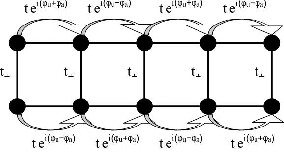
We are now ready to generalize the above treatment to armchair SWNTs. Mapping the interacting honeycomb lattice Hamiltonian for armchair SWNTs onto the two-leg Hubbard model [14], one finds
H0 =
X
ni
(−tc†nic(n+1)i−t⊥c†n1cn2+ H.c.) +U
X
n,i
nn,i,↑nn,i,↓. (46)
While under the mapping,t⊥=tup to 1/Rcorrections [14], we shall allow for t⊥ 6=tto
have better numerical accuracy. Here we also want to include the spin-orbit interaction (28) in this mapping. We use the SO vectors (31), and for simplicity set ~un=1 = 0,
t e
i(φu+φa)t e
i(φu−φa)t e
i(φu+φa)t e
i(φu−φa)t e
i(φu−φa)t e
i(φu+φa)t e
i(φu−φa)t e
i(φu+φa) [image:17.612.79.368.94.249.2]t
¦t
¦t
¦t
¦t
¦Figure 2. Sketch of the two-leg Hubbard ladder including spin-orbit couplings of the type considered here. The arrows indicate the phase for spins up. Spins down have the opposite phase.
term can then be written as
H′ =X
n
i(c†n,1w~n·~σcn+1,1+c
†
n,2w~n+1·~σcn+1,2) + H.c., (47)
consisting of a uniform and an alternating contribution,
c†n,1/2w~n·~σcn+1,1/2 =c†n,1/2w~ ·~σcn+1,1/2±(−1)nc†n,1/2W~ ·~σcn+1,1/2.
The resulting model is studied in the remainder of this section for the special case that bothw~ andW~ are parallel to the uniform magnetic field. Note thatw~ corresponds to the leading SO vector~λin the low-energy theory, whileW~ is related to the subleading vector
~λ′, see equation (36). Moreover, away from half-filling, following standard reasoning,
one may expect that the alternating terms average out. Nevertheless, they will be kept below, but we indeed confirm that in large systems they lead only to small effects. When the above gauge transformation is applied again, we arrive at a two-leg Hubbard ladder (46), but with the on-chain hoppings t carrying both a uniform phase exp(iφu) and an
alternating phase exp(iφa) determined by w~ and W~ , respectively, see figure 2.
Let us first discuss the noninteracting case. ForU = 0, the solution of equations (46) and (47) is straightforward. The eigenenergies are given by (a is the lattice constant)
E1±(kx) = −
q
(2tcos(kxa+σφu))2±4tt⊥cos(kxa+σφu) cos(φa) +t2⊥
E2±(kx) =
q
(2tcos(kxa+φu))2±4tt⊥cos(kxa+φu) cos(φa) +t2⊥
-1.5 -1 -0.5 0.5 1 1.5 kx -3 -2 -1 1 2 3 EHkxL
-3 -2 -1 1 2 3 kx
-4 -3 -2 -1 1 2 3 4 EHkxL
kx E(kx)
kx E(kx)
F B
C E
A E D (b)
0 1 2 3 4 5 6 7 8 9
0 1000 2000 3000 F E D C B A
φφφφa=0,φφφφu=.1 x3
φφφφa=.1,φφφφu=.1
< S + S - + S - S + > [u .a .]
ω
0 1 2 3 4 5 6 7
0 2000 4000 6000 8000 10000
φa=0.1,φu=0
< S +S -+ S -S +> [u .a .] ω (a)
A B C
[image:18.612.74.376.88.427.2]E
fFigure 3. a) ESR spectrum and b) dispersion relation of the non-interacting model for t = t⊥ = 1 and different phase configurations. The dotted (full) lines in (b)
correspond to spins down (up).
there is no ESR interband transition. When the alternating phase is turned on, the folding of the Brillouin zone produces peaks at higher energies. As the parity symmetry is broken, interband transitions are now possible. The opening of the small gap due to the alternating phase is manifested in the splitting seen in peaks A, B and C. The broad structure (F and D) between the highest peaks correspond to transitions between branches with opposite curvature.
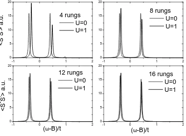
Next we discuss results for U > 0 using the density matrix renormalization group (DMRG) technique [19, 20]. We have used periodic boundary conditions keeping 256 states and the finite-system algorithm. The ESR spectrum (24) at T = 0 has been calculated using the dynamical DMRG technique [21, 22] for a two-leg ladder with uniform phase φu only. Additional small alternating phases φa did not change the
spectrum significantly. In figure 4 we present these results for a quarter filled chain and t⊥ = 1.2 and t = 1. These parameters are used in order to clearly see the effect
-1 0 1 2 0
5 10 15 20
4 rungs
U=0
U=1
<
S
+
S
->
a
.u
.
-1 0 1 2
0 5 10 15 20
8 rungs
U=0
U=1
-1 0 1 2
0 5 10 15 20
12 rungs
U=0
U=1
(
ω-B)/t
<
S
+
S
->
a
.u
.
-1 0 1 2
0 5 10 15 20
16 rungs
U=0
U=1
[image:19.612.79.459.96.373.2](
ω-B)/t
Figure 4. ESR spectra for periodic quarter-filled ladders with a uniform phase
φu = 0.1,t= 1 andt⊥= 1.2.
the cosine bands for system sizes that are multiple of 4. The effect of the correlations mainly consists of a small shift of the peaks, but the double peak spectrum is preserved. Therefore the numerical results lend support to the basic prediction of the analytical low-energy theory, and show that the expected double-peak ESR spectrum is stable with respect to the above-mentioned perturbations.
6. Conclusions
We have reviewed the analysis of the ESR spectrum produced by the spin-orbit coupling in SWNTs. The effective field theory analysis shows that at low energy the SO interaction only acts in the spin sector and the single Zeeman peak, characteristic of a system withSU(2) spin symmetry, splits into two peaks with no broadening. This result relies in an essential way on the property of spin-charge separation characteristic of the Luttinger liquid state realized in the SWNT. Thus the observation of such a splitting would point to this elusive feature.
are appropriate descriptions of this spin problem. The numerical analysis confirms the field theory predictions, including the validity of the approximations involved in their derivation. In addition, it reveals additional structure in the spectrum due to band curvature and higher energy processes, which are not captured by the field theory approach.
Acknowledgments
We thank C.A. Balseiro for the collaboration in the first stage of this work and L. Forr´o for valuable discussions. Support by the DFG under the Gerhard-Hess program, and by the project PICT 99 3-6343 is acknowledged.
References
[1] Dekker C 1999Physics Today52(5)22
[2] Bockrath M, Cobden D H, Lu J, Rinzler A G, Smalley R E, Balents L and McEuen P L 1999 Nature397598
[3] Yao Z, Postma H W C, Balents L and Dekker C 1999Nature402273
[4] Postma H W C, Teepen T, Yao Z, Grifoni M and Dekker C 2001Science29376 [5] Forr´o L and Sch¨onenberger C 2001Topics in Appl. Phys.801
[6] Egger R and Gogolin A O 1997Phys. Rev. Lett.79 5082; Kane C, Balents L and Fisher M P A 1997Phys. Rev. Lett.79 5086
[7] Egger R and Gogolin A O 1998Eur. Phys. J. B3281 [8] Balents L and Egger R 2001Phys. Rev. B64 035310
[9] Gogolin A O, Nersesyan A A and Tsvelik A M 1998Bosonization and Strongly Correlated Electron Systems(Cambridge University Press)
[10] De Martino A, Egger R, Hallberg K and Balseiro C A 2002Phys. Rev. Lett.88206402 [11] Oshikawa M and Affleck I 1999Phys. Rev. Lett.825136
[12] Oshikawa M and Affleck I 2002Phys. Rev. B65 134410 [13] De Martino A and Egger R 2001Europhys. Lett. 56 570 [14] Balents L and Fisher M P A 1997Phys. Rev. B55 11973 [15] Chen G H and Raikh M E 1999Phys. Rev. B 604826 [16] Bonesteel N E 1993Phys. Rev. B 4711302
[17] Ando T 2000J. Phys. Soc. Jpn.691757
[18] Frahm H and Korepin V E 1990Phys. Rev. B42 10553 [19] White S 1992Phys. Rev. Lett.692863; 1993Phys. Rev. B48
[20] Peschel I, Wang X, Kaulke M and Hallberg K 1998Density Matrix Renormalization(Springer) [21] Hallberg K 1995Phys. Rev. B529827