Entropic uncertainty minimum for angle and angular momentum

Entropic uncertainty minimum for angle and

angular momentum

Alison M Yao

1

, Thomas Brougham

2

, Electra Eleftheriadou

1

,

Miles J Padgett

2

and Stephen M Barnett

2

1

Department of Physics, SUPA, University of Strathclyde, Glasgow G4 0NG, UK

2

School of Physics and Astronomy, University of Glasgow, Glasgow G12 8QQ, UK

Received 19 June 2014, revised 8 August 2014 Accepted for publication 15 August 2014 Published 23 September 2014

Abstract

Uncertainty relations are key components in the understanding of the nature of quantum mechanics. In particular, entropic relations are preferred in the study of angular position and angular momentum states. We propose a new form of angle–angular momentum state that provides, for all practical purposes, a lower bound on the entropic uncertainty relation,Hφ+Hm, for any given angular uncertainty, thus improving upon previous bounds. We establish this by comparing this sum with the absolute minimum value determined by a global numerical search. These states are convenient to work with both analytically and experimentally, which suggests that they may be of use for quantum information purposes.

Keywords: entropic uncertainty, orbital angular momentum, quantum information PACS numbers: 03.67.-a, 03.67.Dd, 03.67.Mn, 42.50.-p

(Somefigures may appear in colour only in the online journal)

1. Introduction

Current demands for secure, high-bandwidth communications have resulted in a lot of interest in new protocols in quantum information based on spatial modes carrying orbital angular momentum (OAM) [1–3]. These are defined within an infi -nite-dimensional, discrete Hilbert space and are therefore of considerable interest for quantum information purposes as they have the potential to generate multi-dimensional entan-gled states. The potential for each photon to carry more than one bit of information [4] means that in applications such as quantum key distribution (QKD) not only is the data transfer rate increased in proportion to the number of bits of infor-mation carried by each photon but the security of the protocol is also increased.

Uncertainty relations are of particular importance in the study of quantum-limited measurements as they impose a fundamental limit upon the precision with which conjugate pairs of physical properties of a system can be measured. In other words, the more precisely one property can be

determined, the less well known will be its counterpart. Indeed, the complementarity of incompatible observables is one of the fundamentally distinctive properties of quantum theory [5]. This feature is given quantitative form in the Heisenberg uncertainty principle [6] and its generalization to any pair of observables [7], which place bounds on the pro-duct of the statistical uncertainties or standard deviations for the pair. The uncertainty relation for angular momentum and angular position [8, 9] is much less well-known than the Heisenberg uncertainty relationship for linear position and momentum. It is also a little more complicated as the periodic nature of angular position imposes afinite range of2πon the angle observable and the resultant uncertainty relation has a state-dependent lower bound [7]. In the commonly-chosen range− ⩽π φ<π it can be expressed as [8–11]

Δ Δφm ⩾ 1 − πP −π

2 1 2 ( ) , (1)

where P(−π) is the angular probability density at the boundary of the chosen range.

In this case there are strong reasons for considering other measures of uncertainty. In particular, entropic uncertainties are particularly well suited to states with a dependence on angular position as they avoid the issue of the angle peri-odicity [12]. Among the other advantages of entropic

J. Opt.16(2014) 105404 (6pp) doi:10.1088/2040-8978/16/10/105404

Content from this work may be used under the terms of the

uncertainties is that they distinguish between broad, single-peaked distributions and distributions with two, or more, narrow but widely separated peaks. While both distributions can have a large uncertainty, the latter will have a much smaller entropy. Moreover, entropic uncertainties are well-adapted for quantum communications theory. Indeed, security proofs for QKD are expressed in terms of information or entropy bounds [13]. This suggests that the entropic uncer-tainty relation for angle and angular momentum may find application in secure communications based on OAM [14].

Entropic uncertainty relations place a lower bound on the sum of the entropies associated with the probability dis-tributions for a pair of observables [12,15–19]. An important feature of this lower bound is that it is a constant [16], which is in contrast to the lower bound for the product of standard deviations which is, in general, state-dependent [7]. For linear position and momentum and for angular momentum and angle, for example, the entropic uncertainty relations are [15,17,18]

π

+ ⩾

Hx Hp log (e ), (2) π

+ φ⩾

Hm H log (2 ), (3)

where the entropies are derived from the corresponding wavefunctions:

∫

∫

∫

∑

ψ ψ

ψ ψ

ψ ψ

φ ψ φ ψ φ

= − = −

= −

= − φ

π π

−∞ ∞

−∞ ∞

=−∞ ∞

−

H x x x

H p p p

H m m

H

d ( ) log ( ) ,

d ( ) log ( ) ,

( ) log ( ) ,

d ( ) log ( ) . (4)

x

p

m m

2 2

2 2

2 2

2 2

We note that in the last of these, any2π-integration range may be chosen asψ φ( )is2π-periodic. The explicit values of these entropies depend, of course, on the base of the loga-rithm chosen. Here, for definiteness, we select the natural base so thatlog should be interpreted asloge.

An important point to note is that for linear position and momentum, the lower bound on the entropy sum (2), is satisfied for the Gaussian wavefunctions thatalsosatisfy the equality in the more familiar Heisenberg uncertainty princi-ple. These states are referred to as the intelligent states [12,20] and, indeed, have been demonstrated experimentally [10]. For angular momentum and angle the intelligent states that satisfy the equality in (3) have the form of a truncated Gaussian centred onφ= 0[10]:

⎛ ⎝

⎜ ⎞

⎠ ⎟

ψ =

₍

π_b

₍

π _b

₎₎

− −φ

b

2 erf 2 exp

4 , (5)

Int

2 1

2

whereb=1 (2 )λ anderf ( )x =(2 π)

∫

₀xe−t2dt is the error function [21], as can be seen from the angular probability distribution infigure1. At difference with position and linear momentum, in the case of angle and angular momentum it is possible, for a given Δφ, tofind states for which the uncer-tainty product in (1) islowerthan that for the intelligent states

[11, 22–24]. Such minimum uncertainty states [22], which may be expressed in terms of confluent hypergeometric functions [11] or Mathieu wave functions [23], are possible only because the state-dependent lower bound in (1) takes a yet lower value than the uncertainty product. For the entropic uncertainty (3), in contrast to the linear position and momentum states, only the angular-momentum eigenstates, for whichHm= 0, satisfy the equality. Any state for which the

angular distribution ispeakednecessarily leads to an entropic sum, Hm+Hφ, in excess of log (2 )π . Our aim is then to obtain a stronger lower bound on the sum Hm+Hφ for application when we do not have a flat angular probability distribution,P( )φ =| ( )|ψ φ 2_.

2. Analysis

One motivation for pursuing this specific problem is the existence of quantum communications protocols based on angle and angular-momentum complementarity [25]. It is known that uncertainty principles, both variance based and entropic, impose fundamental limits on quantum information tasks. For example, the ability to perform quantum steering is related to bounds in certain entropic uncertainty principles [26]. Similarly, one can relate the Tsilson bound to the uncertainty principle [27]. Furthermore, many estimates of the secret key rate for QKD depend on bounds for an entropic uncertainty principle [28, 29]. Understanding the minimum uncertainties for angle and OAM is thus important for exploiting OAM for quantum communication. Even approx-imate results are useful, as they can give a strong indication of the optimal performance of tasks such as QKD.

The simplest approach to our problem is tofind a bound given any particular value for the angular standard deviation,

Δφ. This has the added advantage that infixing Δφ we can make a natural connection with existing work on the uncer-tainty principle for angular momentum and angle [10–12].

To obtain a stronger lower bound we require the lowest possible entropic sum,Hm+ Hφ, for a given angular uncer-tainty, Δφ, and tofind the form of the states which achieve this bound. Note, the fact that entropy is concave implies that the minimum uncertainty state will be a pure state [30]. We have not been able to find an analytical form for the lower bound and so have had to rely on a numerical optimisation to find this. There is, however, an excellent analytical approx-imation to the states that reach this lower bound. The states we have found have Gaussian amplitudes in the angular momentum basis:

∑

ψ

ϑ

=

−

=−∞ ∞

−

(

)

1

0, e

e , (6)

oam

a m

am

3 2

2

where a is a real and positive parameter,₁ ϑ _{(0, e}−a₎

3 2 is

the normalisation factor andθ3is an elliptic theta function of the third kind, defined asϑ ( , )u q = ∑∞_{n= −∞}qneinu

3 2

2

Angular momentum and angle are related by a discrete Fourier transform, which leads to the angular wavefunction

⎜ ⎟

⎛ ⎝ ⎞⎠

∑

ψ φ

πϑ

ϑ φ

πϑ

=

=

φ

−

=−∞ ∞

−

−

−

(

)

(

)

( ) 1

2 0, e

e e ,

2, e

2 0, e

, (7)

a m

am im

a

a

3 2

3

3 2

2

where we have re-expressed the sum in terms of its corre-sponding theta function. A straightforward application of the Poisson sum-rule [31] leads to a, perhaps, more physically appealing representation in the form

⎡ ⎣⎢

⎤ ⎦⎥

∑

ψ φ

ϑ

φ π

= − −

− _=−∞

∞

(

)

a a

n

( ) 1

2 0, e

exp 1

4 ( 2 ) . (8)

a _n

3 2

2

We note the similarity between (8) and equation (2.18) of [32].

Our Gaussian distribution of angular momentum states has the form, in the angular representation, of a sequence of overlapping equal Gaussians, peaked at2nπ. Figure1shows the corresponding angular probability distribution in the angular range−πtoπand the comparison with the intelligent states. In this form it is clear that the parametera determines the width of the Gaussians. To be precise,ais proportional to the square root of the width of the Gaussians such that the full width at half maximum (FWHM) of the Gaussians is

a

4 ln 2 . As the parameter a is increased, the width of the Gaussians is increased and, as the angle state is related to the OAM state by (discrete) Fourier transform, the number of states in the OAM distribution decreases accordingly.

The angular uncertainty,Δφ, is defined via

∫

Δφ = φ φ φ

π π

−

P

d ( ), (9)

2 2

where the angular probability distribution isP( )φ =| ( )|ψ φ 2_. For the states (7) we calculate this to be

Δφ π

ϑ

= +

× ∑ −

− ′

−

′=−∞ ≠ ′ ∞

− ′

− + ′

(

)

(

)

m m

3

2 0, e

( 1)

( ) e . (10)

a

m m m m

m m

a m m 2

2

3 2

, ₂

2 2

Equation (10) depends solely on the parametera and so we can calculate the entropic sum (3) as a function of angular uncertainty simply by varying a. Note that as a is increased from 0 towards∞,the angular uncertainty increases from 0 to its limiting value of π 3. The corresponding OAM distribution varies between an almostflat, continuous distribution and a single OAM eigenstate with variance

Δm=0.

It is straightforward to obtain the angular momentum entropy for our Gaussian state:

ϑ Δ

=

(

−

)

+

Hm log 3 0, e 2a 2a m2, (11)

whereΔm2is the angular-momentum variance given by

Δ

ϑ

ϑ

= −

−

−

(

)

(

)

m d

da

1

2 0, e

0, e . (12)

a

a 2

3 2

3 2

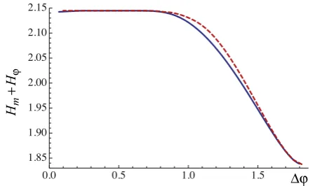
Evaluating the angular entropy presents more of a challenge. We do not have an expression for this in closed form but do have a very good upper bound on its value, which we present in the appendix. It is straightforward, however, to determine the value of Hφ numerically. The result, shown in figure 2, clearly shows a lower entropic uncertainty sum for the Gaussian states than for the intelligent states over a large range of Δφ.

[image:3.595.316.540.64.250.2]

Although we do not have an exact analytical expression for the entropic uncertainty over the entire range of angular Figure 1.The angular probability distribution,P( )φ =| ( )|ψ φ 2_{, in the}

range−π toπfor the overlapping Gaussian states (blue, solid) compared to the truncated Gaussian intelligent states (red, dashed), corresponding to angular varianceΔφ=1.61.

Figure 2.Entropic uncertainty relation,Hm+Hφ, as a function of

Δφfor the intelligent states (red, dashed) and our Gaussian distribution states (blue, solid). Both tend to the limits

π =

e

[image:3.595.315.540.318.451.2]

uncertainty, it is straightforward to obtain limiting forms for large and small values of Δφ. In the limit Δφ tends to its maximum value, π 3, our state becomes the angular momentum eigenstate with m = 0. For this state we have Hm= 0 andHφ= log (2 )π and we reach the global minimum value given in (2). At the other extreme, for small values of

Δφ, our Gaussian peaks become well separated and it suffices to consider only the peak centred atφ =0:

⎛ ⎝

⎜ ⎞

⎠ ⎟

ψ φ ≈ _aπ − − φ

a

( ) (2 ) exp

4 . (13)

2 1

4

In this limit our angle entropy is

π

= φ

H 1 ea

2 log (2 ). (14)

For the angular momentum variance in this limit we find

Δm2= 1 (4 )a _{and our angular momentum entropy is}

⎜ ⎟

⎛ ⎝ ⎞⎠

π

=

H e

a

1

2 log 2 . (15)

m

Thus our entropy sum tends to the valuelog (eπ), which is the value found for the unbounded and continuous obser-vables,xandp. The reasons for this are, of course, that in this limit the angular momentum distribution is broad and slowly varying and so approaches a continuous distribution, and the angle distribution is sharply peaked aroundφ=0 and so is insensitive to the ends of the angle range atφ= ±π.

3. Entropic minimum

It remains to determine how close the entropy sum for our state is to the elusive true minimum value. We have tested this numerically using standard search techniques. Note that we constrain the angular probability of the state to have minima atφ= ±π in order to maximize the rhs of equation (1). We also assume that, like both the intelligent states (6) and our overlapping Gaussian states (8), the angular probability function is symmetric and increases monotonically from the minima to a maximum at φ=0. This, and hence also the corresponding OAM state, are then numerically optimized to minimize the sum Hm+Hφ using an iterative optimisation process. This iteration is repeated several times with a

randomized optimization pathway to confirm that our opti-mization is global.

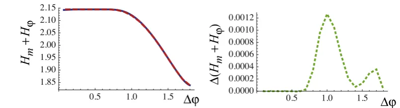
Comparing our numerical result for the entropic sum for our overlapping Gaussian state (6,7) with this global mini-mum, figure 3, we find a very close agreement between the two with the greatest difference, Δ

(

Hm+ Hφ

)

, for Δφ≈1, amounting to only about0.06%. This difference is unlikely to be significant for any but the most sensitive of measurements and suggests that the overlapping Gaussian states provide a practical approximation to the states that minimize the entropic sum for a given angular width.

4. Conclusion

In conclusion, we have presented a new form of angle and orbital angular momentum states which have a Gaussian distribution in angular momentum and consist of a sum of overlapping Gaussians in angle. These are an excellent ana-lytical approximation to the states that minimize the entropic sum, Hm+ Hφ, and thus provide, what is for all practical purposes, a state independent lower bound on Hφ+Hm for any angular width, thereby improving upon previous bounds. We suggest that these states are therefore ideal candidates for use in high-bandwidth, secure quantum information protocols.

Acknowledgements

This work was supported by the UK EPSRC grant EP/I01245/ 1, Challenges in Orbital Angular Momentum, and by the DARPA InPho program through the US Army Research Office award W911NF-10–0395. MJP thanks the Royal Society and the Wolfson Foundation for their support. EE & AMY thank John Jeffers for useful discussions.

Appendix A. Analytic approximation forH_φ

[image:4.595.89.492.66.175.2]

takes the form [33]

∫

φ φ φ φ φ

φ

= π π

−

H P Q P P

Q

[ ( ) ( )] d ( ) log ( )

( ). (A.1)

This quantity has the merit of being always greater than or equal to zero, taking the value zero only if P( )φ =Q( )φ . Hence, if we setP( )φ =| ( )|ψ φ 2 _{then wefind the bound}

∫

φ φ φ

⩽ − φ

π π

−

H d P( ) logQ( ), (A.2)

foranyprobability distributionQ( )φ .

Wefind different upper bounds for different choices of

φ

Q( ). One suitable choice for the probability distribution

φ

Q( )is to use the truncated Gaussian state, which is also the intelligent state for angle and angular momentum [9,10]. This gives:

⎛ ⎝

⎜ ⎞

⎠ ⎟

φ = − −φ

Q Z b

b

( ) ( ) exp

2 , (A.3)

1

2

whereZ b( )= 2πberf(π 2 )b and the positive parameterb is yet to be determined. A straightforward calculation then gives the bound

Δφ

⩽ +

φ

H Z b

b

log ( )

2 , (A.4)

P 2

where Δφ_P2 is the variance associated with the probability distributionP( )φ . Tofind the best bound we simply chooseb so as to minimize our upper bound. To this end we differ-entiate our bound with respect tob tofind the extremum:

⎛

⎝

⎜⎜ ⎞

⎠ ⎟⎟

Δφ

Δφ

+ =

⇒ − =

b Z b b

Z Z

b b

d

d log ( ) 2 0

1 d

d 2 0. (A.5)

P

P 2

2

2

We can write thefirst part of this expression in terms of the variance for the probability distributionQ( )φ :

⎛ ⎝

⎜ ⎞

⎠ ⎟

⎛ ⎝

⎜ ⎞

⎠ ⎟

∫

∫

φ φ

φφ φ

Δφ

= −

= −

= π π

π π

−

−

Z Z

b Z b

b Z b

b

1 d d

1

d exp 2

1

2 d exp 2

2 . (A.6)

Q

2

2

2 2

2

2

It follows that the least upper bound occurs when we choose the two probability distributions,P( )φ andQ( )φ to have the same variance: Δφ_Q2=Δφ_P2=Δφ2_{. Hence, our least upper} bound forHφ, which we denoteΓ, has the form

Γ= Z b + Δφ

b

log ( )

2 , (A.7)

2

wherebis chosen so that Δφ_Q2= Δφ2_.

Wefind that usingΓ in place of Hφgives an excellent approximation to the entropy sum evaluated numerically for

ψ φ( ). Infigure4we compare the exact numerical values for + φ

Hm H , plotted as a function ofΔϕ, withHm+ Γ, whereΓ is evaluated with ΔφQ= Δφ. The solid green line is

+ φ

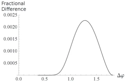
Hm H , while the dashed red line is Hm+ Γ. Figure 4 shows that using Γ in place of Hφ is an excellent approx-imation. This can be shown further by plotting the fractional difference between the two curves plotted in figure 4, as shown in figure 5. We see that the fractional difference between the approximate and exact results is always less than

0.24%.

References

[1] Mair A, Vaziri A, Weihs G and Zeilinger A 2001Nature 412313

[2] Jack B, Yao A M, Leach J, Romero J, Franke-Arnold S, Ireland D G, Barnett S M and Padgett M J 2010Phys. Rev.

A81043844

[3] Leach J, Jack B, Romero J, Jha A K, Yao A M,

Franke-Arnold S, Ireland D G, Boyd R W, Barnett S M and Padgett M J 2010Science329662

[4] Tyler G A and Boyd R W 2009Opt. Lett.34142

[5] Bohr N 1949 Discussion with Einstein on epistemological problems in atomic physicsAlbert Einstein:

Philosopher-Figure 4.A plot comparing the exact numerically calculated value forHm+Hφwith the minimum value forΓ. The solid green line is

+ φ

[image:5.595.319.538.70.216.2]

Hm H, while the dashed red line is for the upper boundΓ.

[image:5.595.317.538.280.424.2]

Scientisted P A Schilpp (Evanston: The Library of Living Philosophers) pp 200–41

[6] Heisenberg W 1927Z. Phys.43172

Heisenberg W 1949The Physical Principles of the Quantum Theory(New York: Dover)

[7] Robertson H P 1929Phys. Rev.34163

Merzbacher E 1970Quantum Mechanics(New York: Wiley) [8] Barnett S M and Pegg D T 1990Phys. Rev.A413427 [9] Galindo A and Pascual P 1990Quantum mechanics I(Berlin:

Springer)

[10] Franke-Arnold S, Barnett S M, Yao E, Courtial J and Padgett M J 2004New J. Phys.6103

Jack B, Aursand P, Franke-Arnold S, Ireland D G, Leach J, Barnett S M and Padgett M J 2011J. Opt.13064017 [11] Pegg D T, Barnett S M, Zambrini R, Franke-Arnold S and

Padgett M J 2005New J. Phys.762

[12] Kraus K 1987Phys. Rev.D353070

[13] Lütkenhaus N 2000Phys. Rev.A61052304

[14] Gibson G, Courtial J, Padgett M J, Vasnetsov M, Pasʼko V, Barnett S M and Franke-Arnold S 2004Opt. Express12

5448–56

[15] Białynicki-Birula I and Mycielski J 1975Commun. Math. Phys.44129

[16] Deutsch D 1983Phys. Rev. Lett.50631

[17] Białynicki-Birula I 1984Phys. Lett.A103253

[18] Białynicki-Birula I and Madajczyk J L 1985Phys. Lett.A 108384

[19] Partovi M H 1983Phys. Rev. Lett.501883

Maassen H and Uffink J B M 1988Phys. Rev. Lett.601103

Ohya M and Petz D 1993Quantum Entropy and Its Use

(Berlin: Springer)

Hall M J W 1995Phys. Rev. Lett.743307

Rojas González A, Vaccaro J A and Barnett S M 1995Phys. Lett.A205247

[20] Aragone C, Guerri G, Salamo S and Tani J L 1974J. Phys. A: Math. Gen.7L149

[21] Gradshteyn I S and Ryzhik I M 2007Table of Integrals, Series, and ProductsChapter 8: Special functions 8th edn ed A Jeffrey and D Zwillinger (New York: Academic) p 887 [22] Jackiw R 1968J. Math. Phys.9339

[23] Hradil Z, R̆ehác̆ek J, Bouchal Z, C̆elechovskýR and Sánchez-Soto L L 2006Phys. Rev. Lett.97243601 [24] Hradil Z, R̆ehác̆ek J, Klimov A B, Rigas I and

Sánchez-Soto L L 2010Phys. Rev.A81014103 [25] Leach J, Bolduc E, Gauthier D J and Boyd R W 2012Phys.

Rev.A85060304(R)

[26] Oppenheim J and Wehner S 2010Science33010702 [27] Chefles A and Barnett S M 1995J. Phys. A: Math. Gen.29L237

[28] Koashi M 2006J. Phys.: Conf. Ser.3698

[29] Nunn J, Wright L J, Söller C, Zhang L, Walmsley I A and Smith B J 2013Opt. Express2115959

[30] Nielsen M A and Chuang I L 2000Quantum Computation and Quantum Information(Cambridge: Cambridge University Press)

Barnett S M 2009Quantum Information(Oxford: Oxford University Press)

[31] Bellman R 1961A Brief Introduction to Theta Functions

Chapter 6: The Poisson summation formula ed F W J Olver, D W Lozier, R F Boisvert and C W Clark (New York: Holt, Rinehart and Winston) pp 7–8

Olver F W J, Lozier D W, Boisvert R F and Clark C W (ed) 2010NIST Handbook of Mathematical FunctionsChapter 20: Theta functions (Cambridge: Cambridge University Press) pp 523–36

[32] R̆ehać̆ek J, Bouchal Z, C̆elechovskýR, Hradil Z and Sánchez-Soto L L 2008Phys. Rev.A77032110 [33] Cover T M and Thomas J A 1991Elements of Information