A CFD analysis of the dynamics of a direct-operated safety relief valve mounted on a pressure vessel

A CFD analysis of the dynamics of a direct-operated safety relief valve mounted

on a pressure vessel

Xueguan Song a,d,⇑, Lei Cui b, Maosen Cao c, Wenping Cao a, Youngchul Park d,⇑, William M. Dempster e

a

School of Electrical and Electronic Engineering, Merz Court, Newcastle University, Newcastle upon Tyne NE1 7RU, UK

b _{School of Civil Engineering and Geosciences, Cassie Building, Newcastle University, Newcastle upon Tyne NE1 7RU, UK} c _{Department of Engineering Mechanics, College of Mechanics and Materials, Hohai University, People’s Republic of China}

d _{Department of Mechanical Engineering, Dong-A University, Busan 604-714, South Korea}

e _{Department of Mechanical and Aerospace Engineering, University of Strathclyde, Glasgow G1 1XJ, UK}

Abstract:

In this study, a numerical model is developed to investigate the fluid and dynamic characteristics of a

direct-operated safety relieve valve (SRV). The CFX code has been used to employ advanced

computational fluid dynamics (CFD) techniques including moving mesh capabilities, multiple domains

and valve piston motion using the CFX Expression Language (CEL). With a geometrically accurate

CFD model of the SRV and the vessel, the complete transient process of the system from valve opening

to valve closure is simulated. A detailed picture of the compressible fluid flowing through the SRV is

obtained, including small-scale flow features in the seat regions. In addition, the flow forces on the disc

and the lift are monitored and analyzed and the comparison of the effects of design parameters, are

examined ; including the adjusting ring position, vessel volume and spring stiffness. Results from the

model allow the fluid and dynamic characteristics of the SRV to be investigated and shows that the

the model shows great potential in assisting engineers in the preliminary design of SRVs, operating

under actual conditions which are often found to be difficult to interpret in practice. .

Keywords:

Direct-operated safety relief valve, pressure vessel, blowdown, CFD, moving mesh

Highlights:

A dynamic CFD analysis of a direct-operated safety relief valve with moving mesh is presented.

Conventional inlet assumption is replaced by a pressure vessel to provide more realistic condition.

The whole operation process of the valve from open to closure is monitored and investigated.

The authors believe that this is the first time that a complete simulation of a SRV has been published

providing detailed insight to the governing flow processes and the ability to accurately quantify valve

dynamics and valve performance only previously available using experimental methods.

1. Introduction

A safety relief valve (SRV) is designed and used to open and relieve excess pressure and to close and

prevent the further flow of fluid after normal conditions have been restored. There are two classical

types of valve that are commercially available: pilot-operated and direct-operated. The pilot-operated

type can maintain a constant pressure in a hydraulic system, such valves are frequently used in

sophisticated hydraulic control systems, but they are expensive and more complex to manufacture

and maintain The direct-operated SRV, also commonly known as a direct-loaded or spring-loaded

SRV, operates with a spring to pre-load and determine motion of the disc of the valve. Due to its simple

configuration and reliable performance, this type of SRV is widely used to provide overpressure

protection in practice.

As SRVs are crucial safety devices in many engineering industries such as the process industries,

petrochemical industries, power plants and nuclear industries it is important to understand the SRVs’

operating characteristics. From the 90’s, with the development of computational methods, the

computational analysis of the complex flows through valves have became more feasible thus leading to

substantial research into the operation and design of SRVs [1-16]. For example, Vu and Wang [1]

investigated the complex three-dimensional flow field of an oxygen SRV during an incident with CFD

(computational fluid dynamics) techniques. The computational result indicated vortex formation near

the opening of the valve which could be matched to the erosion pattern of the damaged hardware.

Francis and Betts [4, 5] studied the pressure distribution on the underside of a commercial SRV disc

and identified the critical backpressure ratio when the SRV was subject to choked compressible flow.

Kim et al. [7] carried out a computational study using the two-dimensional, axisymmetric,

compressible Navier-Stokes equations to simulate the gas flow between the nozzle exit and valve seat.

Ahuja et al. [6, 8] presented a series of high fidelity computational simulations of control valves used in

NASA testing. 3D multi-element framework with sub-models for grid adaption and multi-phase flow

dynamics have been used to investigate the instability that results from valve operation. Dempster et al

[16] also showed by comparison with experimental data the success of relatively simple CFD models

based on two equation turbulence models in predicting the gas flowrate and disc forces for a complex

straight through SRV used in the industrial refrigeration sector. These simulations revealed a rich

variety of flow phenomena such as secondary patterns, hydrodynamic instabilities, turbulent pressure

fluctuations due to vortex shedding, etc. Meanwhile, many researchers started to apply CFD method in

the design and analyze other types of valves like hydraulic control valves and servo valves [17-21]. For

instance, Lisowski and Rajda [20] investigated the pressure loss during flow by hydraulic directional

control valve constructed from logic valves. The undertaken matter is focused on a spool type

directional control valve with pilot operated check valves. Then, they proposed calculation of the forces

associated with the flow using 3D CFD modeling [21]. The force values obtained in the CFD

calculations were compared with those obtained on the test bench. The resulting accuracy has been

proven satisfactory.

However, due to the restriction of CFD tools and computational resources, the numerical

methods used in most of the studies mentioned previously were restricted to steady-state calculations at

various fixed valve openings/lifts, rather than to dynamically simulate the true operation process of

valve opening and closing and the commonly foundvalve chattering conditions. Moreover, most

simulations have not contained all the detailed geometrical effects since two dimensional rather than

Consequently, there has been no systematic study of SRV’s whereby system dynamic effects are

accounted for. The simulation of a blowdown of a pressurized system with its associated connecting

pipe, pressure vessel and SRV requires the interaction of each component to be accounted for.

Completely neglecting the system or vessel is insufficient for deep insight into the performance of

SRVs and the dynamic events which define this such as, the opening time, instability duration and

blowdown.

In this paper, the dynamic analysis of an individual direct-operated SRV by the authors [22, 23] is

extended with similar approaches involving DDM (domain decomposition method), domain interface,

moving grid and CEL (CFX Expression Language) used previously [22] utilized again. Differently

and importantly, instead of giving a static pressure condition at the inlet of the valve, a pressure vessel

is added to provide a relatively real condition, which means that this paper presents an investigation of

a simple system including a pressure vessel and a direct-operated SRV rather than a SRV itself. As a

result, the whole exhausting process from the valve opening to valve re-closure is monitored, and

several important parameters such as displacement/lift of the valve disc, flow mass through the valve,

blowdown of the valve are obtained. The simulation model is then used to demonstrate the usefulness

of the modeling approach to valve designers and operators by investigating parameters of direct interest

to them. In this study the effect of (i) the vessel volume (ii) the spring stiffness and (iii) the adjusting

ring position on the dynamic performance of a SRV is investigated. Additionally an SRV with and

without bellows is also examined to show the versatility of approach. At present generally available

detailed experimental data does not exist to provide an extensive validation of the model however some

valve blowdown results have been used to examine the model accuracy. Compared with the previous

research, this work gives a deeper insight on how a direct-operated SRV mounted on a pressure vessel

really operates to prevent a sudden overpressure incident.

2. Motion of direct-operated SRV

2.1 Direct-operated SRV

Fig. 1 shows the half 3-D model of the direct-operated SRV (manufactured by Jokwang I.L.I Co., Ltd.)

studied in this research. It mainly consists of six parts: valve body, bonnet, nozzle, adjusting ring,

movable valve disc and compressible spring. The operation of this direct-operated SRV is based on a

force balance. When the pressure at inlet is below the set pressure, the resultant force on the disc is

downwards and the disc remains seated on the nozzle in the closed position. As the system pressure

increases to the set pressure, the resultant force decreases to zero gradually. When the inlet static

pressure rises above the set pressure the resultant force reverses, and the disc begins to lift off its seat.

However, as soon as the spring starts to compress, the spring force increases, which requires the system

pressure to continue to rise before any further lift can occur, and for there to be any significant flow

through the valve. The additional pressure above the set pressure is called the overpressure. After

opening, the valve will close when the system pressure drops sufficiently below the set pressure to

allow the spring force to overcome the fluid forces on the disc. The pressure at which the valve re-seats

is the closing pressure, and the difference between the set pressure and the closing pressure as a

fraction of the set pressure is referred to as Blowdown. Figure 2 shows the typical disc travel from the

set pressure to the maximum relieving pressure during the overpressure incident, then to the closing

Spring

Disc (disc and disc holder) Nozzle Body Inlet Adjusting ring Bonnet Out let

Fig. 1. Direct-operated SRV model

Set pressure

Opening

100%

Lift (%)

Reseat

10% Blowdown _{Overpressure 10%}

Closing

Pop

Fig. 2. Relationship between pressure and lift for a direct-operated SRV

2.2 Motion of valve disc

As mentioned above, the motion of the valve Disc is determined based from a force balance at all times.

Deduced from Newton’s second law, the following second-order ordinary differential equation can be

used to simulate the motion of the valve disc.

disc y

spring y

flow

F

G

F

y

m











where constant m is the combined mass of all the moving elements including the disc, disc holder and

stem,



y



spring

F is the

spring force acting on the disc in y direction, and y

flow

F is the flow (viscous and drag) force acting on

combined weight of the moving parts are not large, so the term disc

G is neglected in this research.

Eq. (1) cannot be solved directly, so discretization is needed to transfer the continuous differential

equations into a discrete difference form, suitable for numerical computing. The term on left hand side

of the balance equation can be discretized to include an expression for the velocity of the disc:

t

y

y

y















where the velocity

y



t

y

y

y

t t

_







The displacement of the disc xt also appears in the expression for spring force:

F



K



y



F

where Kspring is the spring stiffness and F0 is the spring pre-load force to establish the required set

pressure. The discrete form of the motion equation is re-assembled, and the disc displacement is

finally isolated as:

2 2 0

t

m

K

t

y

m

t

y

m

F

F

y

































By calculating the fluid induced force and the spring force explicitly at a previous time, the new

position of valve disc after Δt time can be determined and updated.

Since ANSYS CFX cannot read and execute equation (5) directly the equation requires to be

programmed using the ANSYS CFX interpreted language CEL (CFX Expression Language). For the

valve model typical values of the parameters for m, Kspring , Fo and Δt are as follows, m= 0.96 kg,

Kspring=22.3kN/m, Fo=0.96 kN, Δt = 0.0001 sec.

2.3 Moving mesh technique

In ANSYS CFX, the mesh deformation option allows the specification of the motion of nodes on

boundary using CEL. The update of the mesh is handled automatically by CFX at each time step

based on the above mentioned equations. A brief background of the moving mesh model is given as

follows. The integral form of the conservation equation for a general scalar ∅ on an arbitrary control

volume 𝑉, whose boundary is moving, can be written as:

(

)

V V V V

d

dV

u

u

dA

dV

S dV

dt





















 







(6)

Where is the fluid density, uis the flow velocity vector, ug_{is the grid velocity of the moving}

mesh, is the diffusion coefficient, S_{is the source term of}



the control volume. The time derivative term in Eq. (6) can be described using a first-order backward

1

(

)

(

)

V

V

V

d

dV

dt

t







_







where n and n+1 denote the quantity at the current and next time level, respectively. 𝑉𝑛+1is calculated

from

1

n n

dV

V V t

dt

   

(8)

In order to satisfy the grid conservation law, the volume time derivative of the control volume is

computed from

, 1

f

n

m m j j

V

j

dV

u dA u A

dt 





(9)

In the above equation, 𝑛𝑓 is the number of the faces on the control volume, 𝐴⃑⃑⃑ 𝑗 is the j-th face area

vector, the dot product

u

A





_

, on each control volume face is calculate from:

,

j m j j

V

u A

t

  

 ₍₁₀₎

Here, 𝛿𝑉_𝑗 is the volume swept out by the control volume face 𝑗 over timestep ∆𝑡.

The motion of the remaining nodes is determined by the mesh motion model, which is limited to

displacement diffusion. With this model, the displacements applied on domain boundaries are diffused

to other mesh points by solving the equation:











0







Where 𝛿 is the displacement relative to the previous mesh locations and disp _{is the mesh stiffness,}

determining which regions of nodes should move along with the nodes on the boundaries. This

equation is solved at the start of each iteration or time step for transient simulations.

3. CFD analysis of SRV

3.1 Domain decomposition and grid generation

Analyzing the whole system including the SRV and pressure vessel simultaneously was rather difficult

due to their complex internal geometries and the large number of nodes/elements needed to accurately

represent the geometries. Also, symmetry exits only in a single plane allowing some efficiency to be

gained but overall still requiring a three dimensional representation. As far as the moving grids in

ANSYS CFX is concerned, the structural grids must be generated to ensure no element in constructed

with a negative volume/poor quality shape occurs at each iteration while the valve disc is moving. To

this end, the DDM successfully applied in previous work by the authors [21] is utilized. The previous

work is extended by decomposing the whole domain into 4 sub-domains which now include the

pressure vessel, connection pipe between valve and vessel, central domain of valve and the valve vent.

Fig. 3 shows the grid model of the four sub-domains and all of them are meshed with a pure structural

Fig. 3. Structural grids of four sub-domains

3.2 Boundary conditions

After generating the four sub-domains, the whole domain is constructed by connecting them together

via three interfaces as shown in green in Fig. 4. Different from common CFD analysis of a valve, there

is no inlet, instead the pressure in the vessel is set to be the set pressure plus the overpressure of 7% to

supply the flow source. The outlet condition is set to be open, which allows flowing in both directions.

The mesh walls are generally set to be stationary except the surface regions of the disc and the

symmetry plane. The disc motion is specified in the y-direction only while the mesh motion

Fig. 4. Final CFD model and boundary conditions

3.3 Mesh independence and turbulence model comparison

The impact of the mesh fineness and turbulence model in the reproduction of CPU time, flow force on

the disc and air mass flow through the individual RSV is discussed first to find appropriate mesh size

and turbulence model to speed up the simulation as well as diminish the numerical error. The SRV has

the most complex flow conditions and defines the mesh and model requirements. Hence, only the SRV

is used for the mesh size and turbulence model comparison. The inlet condition is set at a given mass

flow of 0.00743Kg/s, and the outlet is set to be open. Three mesh densities have been generated and

distinguished in order of increasing number of elements as coarse, fine and very fine (see Table 2). Fig.

5 shows the mesh model of the SRV used for this study. The calculations adopt five turbulence models

and terminate when the root mean square errors (RMSE) of the velocity components and pressure are

In

te

rf

ac

e

One domain

Interfac

e

DISC

Fig. 5. Mesh model of the direct-operated SRV without pressure vessel

Table 2. Grid information for three types of mesh model

Node Element

Worst mesh number

(Quality < 0.2)

Coarse 29784 36326 80 (0.236%)

Fine 108274 118244 240 (0.207%)

Very fine 276074 258882 336 (0.126%)

Since the mass flow is a boundary condition and therefore known the disc force has been chosen to

judge on the appropriateness of the mesh requirements. Also an investigation on the suitability of the

available turbulence models has been carried out by investigating solutions of a range of two equation

models ; standard k – ε, RNG k-εmodel, the SST model , the k-ω and the BSL model. Fig. 6,

shows the overall results of the study . The SST model, RNG k-εmodel, k-ω model and BSL model

achieve similar results at the finest mesh density. The standard k-εmodel produces lower values of

disc force In addition, the flow force increase as the mesh changes from a coarse mesh to a very fine

mesh. CPU times with different turbulence model and mesh size are compared in Fig. 7, and shows that

the BSL turbulence model costs the most time, and the SST model takes least time when the very fine

mesh is used. For the coarse mesh and fine mesh models, the calculation time of the five turbulence

Dempster et al (16) and Moncalvo et al (9) have investigated the mesh requirements for the simulation

of flows in safety valves. Moncalvo’s work investigated valves similar to this study and both studies

validated computational results against experimental data. Both of these studies showed that mesh

densities where cell sizes were of the order of 0.3-0.5 mm/cell were sufficient to capture both flowrates

and disc flow forces. Moncalvo et al showed that the difference between prediction and experiment for

the mass flows for a number of standard two equation turbulence model were marginal with accuracies

of less than 7% error being achieved. Dempster et al also showed that for both mass flow and disc force

the standard k-εmodel could adequately predict the experimental data to an accuracy of better than

10%. While it is noted that differences do exist between the models examined in this study, in the

absence of detailed disc force measurements more weight has been given the previous studies of

Dempster et al and Moncalvo et al. As a result, the standard k-εmodel is chosen as the turbulence

model and the fine mesh density is used with a total 287415 nodes for the transient study. The validity

of this choice will be discussed later by comparison of vessel blowdown times where experimental data

does exist.

Fig. 6. Flow force with different turbulence model and mesh

Fig. 7. CPU time with different turbulence model and mesh

4. Result and discussion

A simulation of the vessel blowdown transient process was initiated by setting the initial valve

upstream pressure to 7% above the set pressure. This would immediately lead to an opening of the

valve and a flow transient. The results are discussed below.

Figures 8 to 10 show the 3-D flow conditions inside the valve, the Mach number, pressure distribution,

and the vector plots of the velocity fields in the seat region at four time instants (0.005s, 1.001s,

1.8801s and 2.1008s), respectively. The four time instants represent the opening stage, maximum lift

stage, closing stage and closure , respectively.

It can be seen from these figures that, the air accelerates as it flows from the pressure vessel to the

valve inlet. The flow turns supersonic as it rapidly accelerates through the seat region due to the very

narrow gap. In the region between disc and adjusting ring, the flow accelerates further to the maximum

value of approximately Mach 2 condition due to the expansion from sonic flows at the seat. This leads

to the formation of a recirculation zone which causes a reduction in the effective flow area and a rise in

the velocity of the fluid with consequential drop in pressure. As the flow moves from the seat towards

the valve exit flange, the main flow diverges and is deflected outward toward the exit. While on the

opposite side, the fluid flows upwards due to the obstructing valve body and as a result a recirculating

flow is formed inside of the valve body. Due to the multiple direction changes a rotating flow is formed

in the downstream exit passageway. The corresponding pressure distribution also reveals that the main

pressure drop is at the seat region. As the valve is closed, an artificially lift is imposed which separates

the whole field into two pressure fields, where upstream of the seat remains at pressure and

downstream the ambient pressure results.

The changes in disc lift results in significant changes in the flow parameters and the formation of

recirculation zones which reduce the effective flow areas thus affecting the pressure distribution and

the force on the disc.

Fig. 8. Streamline in the valve and vessel

T = 1.0002s

T = 1.8801s

T = 2.1008s

Fig. 10. Velocity vector in the open gap

Fig. 11. Calculated Yplus value on

the disc surfaces at 1.6s

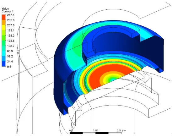
In addition, the Yplus value on the disc surfaces with maximum value of 257.4 is plotted in Fig. 11,

which implies that the mesh size with automatic wall treatment is acceptable to capture the near wall

4.2 Motion of disc and forces on disc

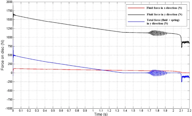
Fig. 12 and 13 show the diagram of the disc lift and forces on it as a function of time for the 2 second

transient process. Figure 12 (b) and (c) are a magnified view of (a), showing a 6 ms opening/pop and

1.0 second closure process, respectively.

From Fig. 9 and Fig. 10, it can be deduced that once the valve has opened, the sudden flow increase in

the seat region leads to a pressure build-up on the front face off the disc which overcomes the spring

force and causes the disc to lift quickly. Within about 6ms, the valve rapidly opens from the initial lift

of 0.6mm to the maximum lift of 8mm. (The small gap of 0.6mm is left to make a continuous flow

field at the starting step.) During this period, the total lift force (∆𝐹𝑦= 𝐹_{𝑓𝑙𝑢𝑖𝑑}𝑦 + 𝐹_{𝑠𝑝𝑟𝑖𝑛𝑔}𝑦 )acting on the

disc sharply increases as shown on Fig 13 b. The force produced by the compressed spring (𝐹𝑠𝑝𝑟𝑖𝑛𝑔)

has little effect compared with the fluid force (𝐹_{𝑓𝑙𝑢𝑖𝑑}) in this period.

Flow is mainly controlled by the opening between the nozzle and the disc until the disc attains the

maximum lift of 8mm. Thereafter, from 6ms to 1.375s, flow is controlled by the inlet bore area rather

than by the area between the seating surfaces. During this period, the valve disc remains at its

maximum lift. As the air is exhausted through the SRV, the average pressure inside of the vessel

decreases proportionally. Consequently, as shown on Fig 13a the lift force also reduces.

At 1.375s into the transient, the net disc force becomes negative and the disc lift starts to decrease from

the maximum lift position. However, while the valve disc begins to move downwards suddenly, the

backlash effect makes the resultant force acting on the valve disc bigger than zero again, i.e., there is a

resultant force opposing the motion, even though this change is very little at that moment. The resultant

force reverse over and over as shown in the figure, but the average lift continues to decrease slightly.

Obviously, each reversal in vibration direction makes the forces acting on the disc more unbalanced,

and in turn, the more unbalanced forces make the vibration stronger. Shown in the figure, the

magnitude of the vibration becomes more and more obvious, although the mean of lift decrease

gradually.

The intensity of the fluid induced vibration will not increase continually due to the continuous pressure

drop, the compressibility of the flowing air and the resistant of the spring. After achieving the

maximum magnitude of vibration, the intensity starts to decrease gradually. Since the process of

vibration delays the closure time of this SRV, when the vibration disappears, i.e., the resultant force doesn’t reverse again, the valve closes rapidly. It shows that, the backlash effect has no significant influence on the motion of the valve disc during this short time. Possible explanation is due to the

pre-compression of spring for compensating the setting pressure. When the overpressure in vessel is

sufficient, the overpressure plays a dominant roles on the vibration, by contraries, when the air pressure

is not sufficient, the pre-compression of spring begins to play a significant role and the left pressure is

not enough to counteract it, so there is no vibration happening.

A small lift of 0.4mm is maintained at closure to ensure the mesh remains continuous. From about 2.1s

on, the valve disc remains at this lowest lift, because the resultant force is negative. A notable low

amplitude oscillation of the force can be seen in Fig 12 at the later stage of the transient. This is

induced by the flowing air and is possibly due to vortex shedding, which is in close proximity to the

(a) Lift from open to re-close

(b) Lift during the open(pop) process

Fig. 12. Lift of valve disc during the whole operation

(a) Forces on valve disc from open to re-close

(c) Forces on disc during re-close

Fig. 13. Lift forces on valve disc

4.3 Flow rate and pressure

Fig. 1 indicates the flow rate through the valve as a function of time ( negative flowrates indicates

valve exit flows). The results show a well-proportioned drop in the flow rate and pressures except that

during the open and closure stage, which is agreement with the real situation. Fig. 15 indicates the

pressure change as a function of time for a location (Monitor point in Fig. 4) and the average absolute

pressure in the vessel. It shows there is a noticeable difference between the average pressure in the

vessel and pressure and reflects the differences in dynamic pressure at the two locations. In addition,

the fluctuation of the pressure at the monitor point during the closure is possibly due to pressure wave

phenomenon when the valve disc alters the direction suddenly.

Fig. 15. Pressure change with time

4.4 Effect of vessel volume

The effect of the vessel volume on the dynamic characteristics of the SRV is investigated, as the valve

is generally mounted on different pressure vessel, pipe or system in various applications. Fig. 16 shows

the previously studied valve mounted on three different pressure vessels, which have volumes of

0.282m3, 0.0707m3 and 0.0353m3, respectively. The computational conditions and settings are as same

as that explained in the former simulation. The only difference is in the calculation time since the

blowdown time is different time for each vessel.

Vessel 1 Vessel 2 Vessel 3

Fig. 16. Valve with different pressure tank

Fig. 17 to Fig. 19 indicates the valve lift, the mass flow through the valve and the average pressure

inside of the vessel along with time for different vessel volumes. As the volume of vessel 2 and

vessel 3 are 1/4 and 1/8 of vessel 1 respectively, the whole operation time of the valve with vessel 2

and vessel 3, as well as the mass flow are approximately 1/4 and 1/8 of those with vessel 1, respectively.

The same pressures as shown in Fig. 19 implies that the blowdown of the direct-operated SRV is an

inherent characteristics of the valve, which does not depend on the volume of the pressure vessel it is

mounted on. It is also noted that the oscillations of the valve disc movement respond differently to the

depressurization rate with the effect diminishing at faster rates. This is likely to be due to the inertia

Fig. 17. Lifts of valves with different vessel

Fig. 18. Mass flow through the valves

4.6 Effect of adjusting position

The valve blowdown value , ie the pressure as a % of the set pressure at which the valve closes is one

of the most important performance criteria for a SRV. In the valve studied here it can be adjusted by

changing the position of Adjusting Ring (see fig 1). The adjusting ring alters the flow at the seat which

results in a change to the pressure distribution and force on the lower face of the disc. The effect of the

adjusting ring position on the Blowdown is presented below. As shown in Fig. 20, the adjustment of the

ring alters the geometry at the top plane of the nozzle. Table 3 and Fig. 21 compare the blowdown

values obtained from the CFD simulation and physical experiments. As seen, the blowdown is large

when the adjustment h is small, and decreases as h increases. This is because the lower values of h

results in a higher pressure distribution on the disc face producing higher flow forces. The vessel

pressure must reduce to a lower value of pressure to allow the valve to close leading to greater

Blowdown value. As the ring is altered to produce larger value of h the pressure distribution changes

resulting in lower flow forces which allows the valve to close at higher vessel pressures. However, the

effect is limited due and the blowdown does not change past a threshold value. of adjustment due to the

limiting changes to the flow.

Disc A d ju st in g R in g N o zz le Inlet

h

h= 1.428, 2.063, 2.4, 2.813 (mm)

Rotation

Fig.20. Comparison of adjusting ring positions

Table 3. Blowdown comparison for different adjustment

Position h (mm)

Blowdown

(%)[CFD]

Blowdown (%)

[Experiment]

Error (%)

1 1.482 37.45 30.68 11.194

2 2.063 30.95 29.12 6.284

3 2.40 27.91 25.24 10.578

Fig. 21. Blowdown at three adjustments

Table 3 and Fig 21 also show a comparison between the predictions and experimentally determined

values of blowdown for four positions of the Adjusting Ring. The predictions show promising results

and are within 11% of the experiments. This blowdown comparison reflects that ability of the model to

capture the mass flows , the flow forces and the disc dynamics during the transient process. Four

different ring positions require the flow field to be predicted adequately during the closure process for

four different geometrically different disc geometries and reflect the accuracy of the model during the

closure process. These error values are deemed acceptable and consistent with the expected

accuracies for mass flow and force suggested by Moncalvo et al [9] and Dempster et al [16] discussed

earlier.

4.5 Effect of spring stiffness

Besides the position of the adjusting ring, the spring stiffness has a significant effect on the closing

dynamics. The effect of four different springs are studied with spring stiffness’s, K1=22.3N/mm,

K2=55.8N/mm, K3=111.7N/mm, K4=167.5N/mm. Vessel 3 is chosen to be the pressure vessel used for

this study to reduce the computational time. Fig. 22 to Fig. 24 illustrate the lift of the valve, mass flow

through the valve and the pressure inside of the vessel. It can be seen from Fig 22 that, for the lower

stiffness springs, K1 and K2, the disc reaches its maximum lift rapidly, and closes relatively smoothly

initially with a more rapid closure over the lift range 4mm to 0mm. However, when the stiffness of the

spring becomes larger, i.e. K3 and K4, the valve does not reach the maximum lift due to the larger

spring force acting on the disc and the valve drops to full closure slowly and gradually. In addition it is

evident from Fig 23 that for spring stiffness K4 the valve does not reach its maximum design massflow

due to the valve not opening fully. Also, due to the difference of the closing time, the blowdown

values for each spring have significant difference as shown in Fig. 2.

Fig. 23. Mass flow for different spring stiffness

Fig. 24. Pressure left for different spring stiffness

4.6 Effect of bellows

The pressure downstream of a direct operated valve can influence the forces on the disc and is caused

by the pressure build up due to flow effects or elevation of the pressure in components downstream of

the valve. This backpressure effect limits the operation of the valve but can be removed by the

inclusion of a balanced bellows to isolate the back face of the disc from the valve exit pressure. Typical

valves with and without balanced bellows are shown in Fig. 25. The effect of adding a bellows is

studied here using the CFD model. Fig. 26 and Fig. 27 compare the lift of the valve disc and pressure

effect on the valve opening process, however, the inclusion of a bellows affects the valve closing

process and final pressure in the vessel. This is because with a bellows, the net force on the disc is

dominated by the front disc face pressure and the spring which will produce a higher flow force

compared to excluding the bellows which result in a backpressure acting on the disc and will reduce the

net flow force. Thus, a lower pressure is required in the vessel before the valve begins to close which

requires the transient to be extended and will lead, in this case to a lower blowdown value.

Fig. 25. Direct-operated SRV with bellows (left) and without bellows (right)

Fig. 27. Pressure change for valves with and without bellows

5. Conclusions

This study describes a CFD investigation into the dynamic simulation of a direct-operated SRV valve

mounted on a pressure vessel. The valve dynamics are modeled using a 3-D moving mesh CFD

approach to predict the mass flows and valve disc force combined with a simple one degree of freedom

model for the disc to determine the valve response during the opening and closing process. The use of

the model suggests the following conclusions can be made.

a. The combined CFD model with a standard k-e turbulence flow model and a single degree of

freedom model for the disc can satisfactorily capture the main dynamic events of the opening

b. The combined model can predict valve blowdown to within 11% of actual results providing

some confidence in the approach.

c. Examination of a number of design and operational parameters has shown the versatility and

usefulness of the approach.

The model used in this study y has used simplifying assumptions which neglect damping effect of the

valve/spring, which may lead to over prediction of disc oscillation during the closure process. In

addition more detailed measurements of disc motion, mass flow and forces during the transient are

required for full validation of the combined model. In future work, such limitations require to be

corrected.

ACKNOWLEDGEMENT

This work was supported byTechnicalCenter for High-Performance Valves from the Regional

Innovation Center (RIC) Program of the Ministry of Knowledge Economy (MKE).

Reference:

[1] Vu B, Wang TS. Navier-Stokes flow field analysis of compressible flow in a high pressure safety

relief valve. Applied Mathematics and Computation 1994;65:345-353.

[2] Betts PL, Francis J. Pressures beneath the disc of a compensated pressure relief valve for

gas/vapour service. Proceedings of the Institution of Mechanical Engineers, Part E: Journal of

Process Mechanical Engineering 1997;211: 285-289.

[3] Mokhtarzadeh-Dehghan MR, Ladommatos N, Brennan TJ. Finite element analysis of flow in a

[4] Francis J, Betts PL. Modelling incompressible flow in a pressure relief valve. Proceedings of the

Institution of Mechanical Engineers, Part E: Journal of Process Mechanical Engineering

1997;211:83-93.

[5] Francis J, Betts PL. Backpressure in a high-lift compensated pressure relief valve subject to single

phase compressible flow. Journal of Loss Prevention in the Process Industries 1998; 11:55-66.

[6] Cavallo PA, Hosangadi A, Ahuja V. Transient Simulations of Valve Motion In Cryogenic Systems.

In: Proceedings of 35th AIAA Fluid Dynamics Conference and Exhibit; Toronto; 2005.

[7] Kim HD, Lee JH, Park KA, Setoguchi T, Matsuo S. A study of the gas flow through a LNG safety

valve. Journal of Thermal Science 2006;15:355-360.

[8] Ahuja V, Hosangadi A, Shipman J, Daines R, Woods J. Multi- element unstructured analyses of

complex valve systems. Journal of fluids engineering 2006;128:707-716.

[9] Moncalvo D, Friedel L, Jörgensen, B, Höhne T. Sizing of Safety Valves Using ANSYS CFX-Flo®.

Chemical engineering & technology 2009;32:247-251.

[10] Chabane S, Plumejault S, Pierrat D, Couzinet A, Bayart M. Vibration and chattering of

conventional safety relief valve under built up back pressure. In Proc. 3rd IAHR International

Meeting of the Workgroup on Cavitation and Dynamic Problems in Hydraulic Machinery and

Systems, Czech Republic; 2009. P. 1-14.

[11] Beune A, Kuerten JGM, Schmidt J. Numerical calculation and experimental validation of safety

valve flows at pressures up to 600 bar. AIChE Journal 2011;57: 3285-3298.

[12] Bernad SI, Susan-Resiga R. Numerical model for cavitational flow in hydraulic poppet

valves. Modelling and Simulation in Engineering 2012;10.

Two-Phase Flow Conditions (PVP-2011-57896). Journal of Pressure Vessel Technology

2013;135;011305-1-011315-11

[14] Schmidt J, Peschel W, Beune A. Experimental and theoretical studies on high pressure safety

valves: sizing and design supported by numerical calculations (CFD). Chemical engineering &

technology 2009;32: 252-262.

[15] Pan XD, Wang GL, Lu ZS. Flow field simulation and a flow model of servo-valve spool valve

orifice. Energy Conversion and Management 2011;52: 3249-3256.

[16] Dempster WM, Lee CK, Deans J. Prediction of the flow and force characteristics of safety relief

valves ,ASME Pressure Vessels and Piping Division Conference, ICPVT 11,July 23-26 2006

Vancouver

[17] Halimi B, Kim SH, Suh KY. Engineering of combined valve flow for power conversion

system. Energy conversion and management 2013;65: 448-455.

[18] Chattopadhyay H, Kundu A, Saha BK, Gangopadhyay T. Analysis of flow structure inside a spool

type pressure regulating valve. Energy Conversion and Management 2012;53:196-204.

[19] Li BR, Gao LL, Yang G. Evaluation and compensation of steady gas flow force on the

high-pressure electro-pneumatic servo valve direct-driven by voice coil motor. Energy Conversion

and Management 2013;67:196-204.

[20] Lisowski E, Rajda J. CFD analysis of pressure loss during flow by hydraulic directional control

valve constructed from logic valves. Energy Conversion and Management 2013;65:285-291.

[21] Lisowski E, Czyżycki W, Rajda J. Three dimensional CFD analysis and experimental test of flow

force acting on the spool of solenoid operated directional control valve. Energy Conversion and

[22] Song XG, Wang L, Park YC. Transient analysis of a spring-loaded pressure safety valve using

computational fluid dynamics (CFD). Journal of pressure vessel technology 2010;132: 1-5

[23] Song XG, Park YC, Park JH. Blowdown Prediction of Conventional Pressure Relief Valve with

Simplified Dynamic Model. Mathematical and Computer Modelling 2013;57: 279-288.