Modelling the joint distribution of competing risks survival times using copula functions

City, University of London Institutional Repository

Citation: Kaishev, V. K., Haberman, S. and Dimitrova, D. S. (2005). Modelling the joint

This is the unspecified version of the paper.

This version of the publication may differ from the final published

version.

Permanent repository link: http://openaccess.city.ac.uk/2295/

Link to published version: Actuarial Research Paper No. 164

Copyright and reuse: City Research Online aims to make research

outputs of City, University of London available to a wider audience.

Copyright and Moral Rights remain with the author(s) and/or copyright

holders. URLs from City Research Online may be freely distributed and

linked to.

Faculty of Actuarial

Science

and

Statistics

Modelling the joint distribution of

competing risks survival times

using copula functions.

V. K. Kaishev S. Haberman

D.

S.

Dimitrova

Actuarial Research Paper No. 164

October 2005

ISBN 1 901615-89-8

Cass Business School

106

Bunhill

Row

London

EC1Y

8TZ

competing risks survival times

using copula functions

by

Vladimir K. Kaishev

*

, Dimitrina S. Dimitrova and Steven

Haberman

Cass Business School, City University, London

Abstract

The problem of modelling the joint distribution of survival times in a competing risks model, using copula functions is considered. In order to evaluate this joint distribution and the related overall survival function, a system of non-linear differential equations is solved, which relates the crude and net survival functions of the modelled competing risks, through the copula. A similar approach to modelling dependent multiple decrements was applied by Carriere (1994) who used a Gaussian copula applied to an incomplete double decrement model which makes it difficult to calculate any actuarial functions and draw relevant conclusions. Here, we extend this methodology by studying the effect of complete and partial elimination of up to four competing risks on the overall survival function, the life expectancy and life annuity values. We further investigate how different choices of the copula function affect the resulting joint distribution of survival times and in particular the actuarial functions which are of importance in pricing life insurance and annuity products. For illustrative purposes, we have used a real data set and used extrapolation to prepare a complete multiple decrement model up to age 120. Extensive numerical results illustrate the sensitivity of the model with respect to the choice of copula and its parameter(s).

Keywords: dependent competing risk model, disease elimination, failure times, overall survival function, copulas, spline function

1. Introduction

The competing risks model with independent failure time random variables has been considered by a number of authors in the (bio)statistical, econometric, medical, demographic and actuarial literature and the list of references, scattered throughout these areas, is extensive. We will mention here the textbooks due to David and Moeschberger (1978), Elandt-Johnson and Johnson (1980) and Bowers et al. (1997) and also the recent papers by Salinas-Torres et al. (2002) and Bryant and Dignam (2004), and also by Zheng and Klein (1994, 1995) where statistical methods for estimating related survival functions are considered.

The competing risk model, alternatively referred to as multiple decrement model, has also been considered under the assumption of dependence between the failure times in the early work of Elandt-Johnson (1976). Later, Yashin, Manton and Stallard (1986) considered conditional independence of the times to death, given an assumed stochastic covariate process. More recently, Carriere (1994) and Escarela and Carriere (2003) modelled dependence between two failure times by a two dimensional copula. Carriere (1994) has used a bivariate Gaussian copula to model the effect of complete elimination of one of two competing causes of death on human mortality. However, the mortality data used by Carriere (1994) was not complete with respect to older ages and therefore, it was not possible to calculate such important survival characteristics as expected life times and life annuities and draw relevant conclusions. In Escarela and Carriere (2003), the bivariate Frank copula was fitted to a prostate cancer data set. The issues of identifiability of marginal survival functions in a copula based competing risk model have been considered by Tsiatis (1975), Prentice et al. (1978), Heckman and Honore (1989) and later by Carriere (1994).

In this paper, we will consider further the copula based competing risk model, studied by Carriere (1994). We will investigate its sensitivity with respect to alternative choices of bivariate copula and its parameter(s). For this purpose, we have closed the survival model by applying a method of spline extrapolation up to a limiting age 120 and have explored the Gaussian copula, the Student t-copula, the Frank copula and the Plackett copula as alternatives. As discussed in Section 3, these copulas allow for modelling the dependence between failure times within the entire age range, from perfectly negative, to perfectly positive dependence. They belong to different families with different properties, and hence are appropriate for studying the sensitivity of the model. We develop this methodology, so as to model the effect of both partial and com-plete elimination of a cause of death on human mortality. The construction of multiple decrement tables, derived from the multivariate competing risk model is also addressed.

Since most real life applications are truly multivariate, i.e., there are more than two mutually dependent competing causes of decrement, our further goal here will be to extend and explore the applicability of the model to the multi dimensional case. This is in general a difficult task, since the bivariate copula theory does not extend to the multivariate case in a direct way. Although some fundamental results (e.g. Sklar's theorem) hold, constructing multivariate copula is related to some open problems, e.g., there is no unique multivariate dependence measure which extends the (bivariate) definitions of Kendall's t and Spirman's rS and the

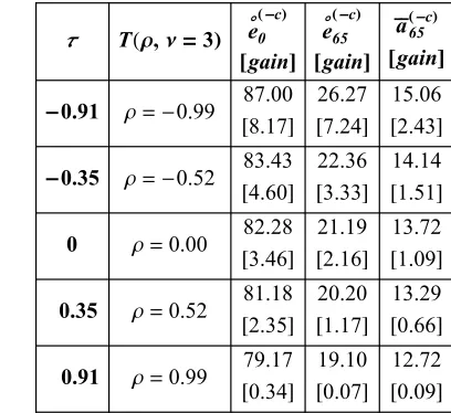
computational complexity increases. This makes multivariate copula applications less appealing. Here we have explored the applicability of the four dimensional Gaussian, t- and Frank copula to model the joint distribution of four competing risks, heart diseases, cancer, respiratory diseases and other causes of death, grouped together. The effect of simultaneously removing one, two or three of them on the overall survival, on the life expectancy at birth and at age 65, and on the value of a life annuity, which are important in pricing life insurance products, is also studied.

imple-ment the proposed methodology. In Section 4, we have addressed the problem of selecting an appropriate copula function and estimating its parameter(s). Then, in Section 5, we describe how, given some estimates of the crude survival functions and an appropriately selected copula, one can evaluate the net survival functions for the corresponding competing risks, by solving a system of nonlinear differential equations. In Section 6, we show how, by introducing an appropriate function, one can modify the net survival functions, obtained as solutions of the system of differential equations, so as to model not only complete but also partial elimination of any of the causes of death in the model. Finally, in Section 7 the proposed methodol-ogy is applied to the general US population, using cause specific mortality data set, provided by the National Center for Health Statistics(NCSH) (1999). Extensive numerical results and graphs illustrate the effect on survival of complete (partial) elimination of cancer, as a cause of death, in a two dimensional decrement model, and the elimination of any combination of heart diseases, cancer and respiratory diseases in a four variate model. Details of how the raw mortality data was used to obtain the crude survival functions and the method of smoothing and extrapolating the latter up to age 120 are provided in the Appendix.

2. The dependent multiple decrement model

We consider a group of lives, exposed to m competing causes of death, i.e., to m causes of withdrawal from the group. It is assumed that each individual may die from any single one of them causes. To make the problem more formally (mathematically) tractable it is assumed that, at birth, each individual is assigned a vector of times T1, ...,Tm, 0§Tj< ¶, j=1, ...,m, representing his/her potential lifetime, if he/she were

to die from each one of the m diseases. Obviously, the actual lifetime span is the minimum of all the

T1, ...,Tm. Thus, it is clear that under this model the lifetimes T1, ...,Tm are unobservable, and we can only

observe the minHT1, ...,TmL. In the classical multiple decrement theory the random variables T1, ...,Tm are

assumed independent, whereas here we will be interested in their joint distribution

(1)

FHt1, ...,tmL=PrHT1§t1, ...,Tm§tmL

and more precisely in the multivariate, joint survival function

(2)

SHt1, ...,tmL=PrHT1>t1, ...,Tm>tmL

which is considered absolutely continuous and where tj¥0, for j=1, ...,m.

As pointed out by a number of authors (see e.g. Hooker and Longley-Cook (1957), Carriere (1994), Valdez (2001)), decrements in many real life actuarial applications tend to be dependent and hence, the random variables T1, ...,Tm will be considered stochastically dependent and also non-defective, i.e., PrHTj< ¶L=1.

The overall survival of an individual, under our model assumptions, is defined by the random variable minHT1,T2, ...,TmL, and so we will be interested in the overall survival function, which we define as

HtLªSHt, ...,tL=PrHT1>t, ...,Tm>tL=PrHminHT1, ...,TmL>tL, where t¥0. We are interested in the

effect of elimination of a cause of death on the overall survival. Of course, since the data which we will use are in the form of counts of age specific deaths from each of m competing causes of death, we could investi-gate how elimination of a cause of death affects the joint survival function (2). By eliminating a cause of death, we mean that a cure for this particular cause of death (say, indexed by j) is found in the future, which will result in postponing the corresponding lifetime, Tj, to infinity, i.e., we assume nobody will die from this

cause of death in the future. Thus, we assume that we may remove the j-th cause from the set of m causes, operating in the multiple decrement model. Mathematically, this is equivalent to assuming that the event

8Tj>t< will occur with probability 1 for any value t¥0, i.e., PrHTj= ¶L=1. Thus, we may consider the

FHt1, ...,tj-1,tj+1, ...,tmL=PrHT1§t1, ...,Tj-1§tj-1,Tj+1§tj+1, ...,Tm§tmL.

The overall survival function then becomes

(3) PrHT1>t, ...,Tj-1>t,Tj+1>t, ...,Tm>tL=PrHminHT1, ...,Tj-1,Tj+1, ...,TmL>tL,

i.e., we are considering the overall survival function with the j-th cause of death removed, and we will simply denote this by H-jLHtLªSH-jL_{Ht, ...,tL. Our major goal in this investigation will be to find a} representa-tion of the latter survival funcrepresenta-tion which will allow us to estimate it and thereby measure the effect of removing a cause of death. As we will see in the following sections, one such representation is through the use of a suitable copula function.

Let us now introduce the notion of the crude survival function. The crude survival function SHjL_{HtL is defined} as the survival function with respect to the j-th cause of death, due to which death actually occurs, i.e.,

(4)

SHjL_HtL=PrHminHT

1, ...,TmL>t, minHT1, ...,TmL=TjL

The survival function SHjL_{HtL is called crude, since it reflects the observed mortality of an individual and} hence, may be estimated, from the observed mortality data of a population, as will be illustrated in Section 3. In the biostatistics literature the crude survival function SHjL_{HtL is sometimes called the subsurvival function} or the cumulative incidence function (see e.g. Bryant and Dignam, 2004).

It is not difficult to see that

(5)

SHt, ...,tL=SH1L_HtL+....+SHmL_HtL,

since the events minHT1, ...,TmL=Tj, j=1, ...,m are mutually exclusive.

This obviously suggests that the distributions in (4) are degenerate and that the crude survival functions are such that SHjL_{H0L<1, j=1, ...,m.}

Let us now define the net survival function S'HjL_{HtL as S}'HjL_HtL=PrHT

j>tL. Note that S'HjLHtL is the marginal

survival function, due to cause j alone, associated with the joint multivariate survival function (2). Thus, we can view (1) as a multivariate distribution with marginal distribution functions F'HjL_HtL=1-S'HjL_HtL,

j=1, ...,m. As we will see, S'HjL_{HtL are the target quantities in our study since, if we know them we can} identify and calculate the joint survival function SHt1,t2, ...,tmL and hence, evaluate the overall survival

function SHt, ...,tL, under some appropriate assumptions. The classical model of independence of the r.v.s

T1,T2, ...,Tm implies that

SHt1, ...,tmL=S'H1LHt1Lä...äS'HmLHtmL.

When we consider the case of stochastic dependence between the causes of death, apart from knowing the marginals F'HjL_{HtL we will need to impose a certain dependence structure, in order to characterize the joint} distribution of the r.v.s T1,T2, ...,Tm. One way of doing so is to use copulas. Thus, to obtain the joint

survival function SHt1, ...,tmL, one would need to select a suitable copula, which mixes (couples) the net

Copulas have recently attracted considerable attention as a tool for modelling dependence in a wide range of applications in finance, insurance, and economics. In Section 3, we introduce the required background material on copulas and recall the Gaussian copula and the t-copula from the Elliptical class of copulas, the Frank copula from the Archimedean family, and also the Plackett copula. We provide also some general comments on the choice of copula, appropriate for our modelling purposes. For further details on copulas, the interested reader is referred to Georges et al. (2001), Frees and Valdez (1998), and Embrechts et al. (2001), and the books by Nelsen (1999), Joe (1997) and Cherubini et al. (2004).

3. Copulas and their properties

Copulas provide a very convenient way to model and measure dependence between failure time random variables since they give the dependence structure which relates the known marginal distributions of the failure times to their multivariate joint distribution. In order to see this, we first provide a short introduction on copulas.

If we assume that u=Hu1, ...,umL', ujœ@0, 1D, an m copula CHuL is conventionally defined as a multivariate

cumulative distribution function with uniform margins. A probabilistic way to define the copula is provided by the theorem of Sklar (1959). Let X1, ..., Xm be random variables with continuous distribution functions

F1, ...,Fm, and survival functions S1=1-F1, ...,Sm=1-Fm respectively, and joint distribution and

survival functions HHx1, ...,xmL and SHx1, ...,xmL. Sklar's theorem states that if H is an m-dimensional d.f.

of the random vector HX1, ...,XmL with continuous marginals F1, ...,Fm, then there exist a unique m copula

C, such that for all x in m

(6)

HHx1, ...,xmL = CHF1Hx1L, ...,FmHxmLL

and conversely, if C is an m copula and F1, ...,Fm are d.f.s, then H is an m-dimensional distribution

function with marginals F1, ...,Fm. Hence, the copula of the random vector HX1, ..., XmL~H is the

distribu-tion funcdistribu-tion of the random vector HF1HX1L, ...,FmHXmLL. Thus, following (6), one can construct a

depen-dence structure, i.e., an m-dimensional d.f. H by appropriately choosing a set of marginals F1, ...,Fm and a

copula function C. In order to construct a copula function, a corollary of Sklar's theorem can be applied, according to which a copula can be represented as an m-dimensional distribution function with continuous marginals, evaluated at the inverse functions F1-1Hu1L, ...,Fm-1HumL, defined as Fi@Fi-1HxiLD=xi , i.e.,

(7)

CHu1, ...,umL= HHF1-1Hu1L, ...,Fm-1HumLL .

By using the probability integral transformation, Xj# FjHXjL=1- SjHXjL as a result of which SjHXjL has a

uniform distribution on @0, 1D, it is easily verified (see Sklar, 1996) that Sklar's theorem, given by (6) can be restated to express the multivariate survival function SHx1, ...,xmL via an appropriate copula Cêêê called the

survival copula of HX1, ...,XmL. Thus,

(8)

SHx1, ...,xmL = CêêêHS1Hx1L, ...,SmHxmLL.

The survival copula, relates the marginal survival functions S1Hx1L, ...,SmHxmL to the multivariate joint

survival function SHt1, ...,tmL in much the same way as the copula C relates the marginal distribution

functions to the multivariate distribution function.

Let us note that the copula C and the survival copula Cêêê of a random vector HX1, ...,XmL do not in general

coincide. In order to see how the survival copula is expressed through its corresponding copula, we refer to Nelsen (1999) and Georges et al. (2001). The survival copula, Cêêê, in (8) can be expressed through its copula,

C, derived on the basis of specific distributions F1, ...,Fm, using (7). However, since CêêêHuL is a copula, one

This will be the approach taken here in modelling the joint survival function of competing risk survival times.

We conclude this description of the general background on copulas by recalling the fundamental Fréchet-Ho-effding bounds inequality which holds with respect to every m-dimensional copula function. To capture its importance we will first give its bivariate version, i.e.,

(9) maxHu1+u2-1, 0L§CHu1,u2L§minHu1,u2L.

where the maximum and the minimum in (9) are correspondingly the lower and upper Fréchet-Hoeffding bounds which themselves are copulas. Following (9), in order that the random variables X1,X2 with a

copula function CHu1,u2L be perfectly negatively (positively) dependent, CHu1,u2L needs to coincide with

the lower (upper) Fréchet-Hoeffding bound. The r.v.s X1,X2 are independent iff their copula is equal to the

product copula, i.e., iff CHu1,u2L=u1u2. It can then be shown that (9) generalizes to the multivariate case as

maxHu1+...+um-m+1, 0L§CHu1, ...,umL§minHu1, ...,umL.

Many popular families of copulas depend on a set of parameters, not related to the parameters of the mar-ginal distributions. This is due to the fact that copulas are invariant under increasing transformations of their corresponding random variables, hence are "scale-invariant". In order to model the full range of dependence, from perfect negative dependence, through independence, to perfect positive dependence, the copula parameters should be set so that the copula CHu1,u2L attains correspondingly, its lower Fréchet-Hoeffding

bound, coincides with the product copula, and attains its upper Fréchet-Hoeffding bound. Copulas which allow this are called comprehensive copulas (see Deheuvels, 1978). Since it is meaningful to investigate the full range of dependence between survival time r.v.s, it is desirable to use comprehensive copulas in model-ling the dependence of competing causes of death. So, this is one of the important criteria in selecting the appropriate copula, i.e., it should be able to reproduce dependence throughout the whole range.

Sklar's theorem and its corollary, given by (7), provide a convenient tool for constructing copulas. Examples of such copulas are the multivariate Gaussian and Student t- copulas which belong to the wider class of Elliptical copulas. However, there are other ways of constructing copulas. For example, the popular Archimedean copulas are constructed as

(10)

CA_Hu

1,u2L= f-1HfHu1L+ fHu2LL.

where f is a continuous, convex function called a generator, such that fH1L=0 and fH0L= +¶ (see e.g. Nelsen, 1999). In what follows, we will introduce and use the Frank copula as one of the only two known comprehensive, bivariate Archimedean copulas. In addition, we will also use the Plackett copula, which does not belong to the Elliptical or to the Archimedean family but is comprehensive and hence, suitable for use in the competing risk model. For these and other properties of Frank and Plackett copulas we refer to Section 3.4 and also to Nelsen (1999).

3.1 Measures of association

We will consider here the standard dependence (concordance) measures, Kendall's t and Spearman's rS,

and the tail dependency as measures of association between two random variables X and Y. These measure are related to the copula since the latter is an expression of the stochastic relationship between X and Y

within the entire range of values which the variables can take. It is not difficult to show that

(11)

rSHX,YL= 12‡ 0

1 ‡

0 1

CHu1,u2L „u1 „u2 -3

(12)

tHX,YL= 4_‡

0 1

‡ 0

1

CHu1,u2L „u1 „u2 -1

(see e.g. Cherubini et al., 2004), i.e., knowing the copula CHu1,u2L of a pair of r.v.s X and Y one can

evaluate these two measures of rank correlation using (11) and (12). Let us note that the sample versions of

rS, and t are known in statistics as rank correlation coefficients. For further properties of rS and t we refer

e.g., to Nelsen (2001). If Hx1,y1L and Hx2,y2L are two observations on the random vector HX,YL then they

are said to be concordant or discordant if Hx1-x2LHy1-y2L>0 or Hx1-x2LHy1-y2L<0 respectively.

Another, important measure of dependence, which can be described as a measure of concordance in the tails of two r.v.s X and Y, is given by the upper and lower tail dependence coefficients

lLHX,YL= lim

pØ0PrHY§yp»X §xpL.

lUHX,YL= lim

pØ1PrHY>yp»X >xpL.

where xp and yp denote the lower p-quantiles of X and Y, i.e., PrHX §xpL=p and PrHY §ypL=p. It can

be shown that the coefficients of lower and upper tail dependence for the Elliptical copulas are equal (see e.g. Embrechts et al., 2001).

3.2 The Gaussian copula

We will first introduce the Gaussian copula. Let the random variables X1, ..., Xm be standard normally

distributed, i.e., Xi~ NH0, 1L, i=1, ...,m and let also the random vector HX1, ...,XmL have a standard

m-variate normal distribution with correlation matrix R=8Rij<, i, j=1, ...,m. Clearly, Rij are the linear

correlation coefficients of the corresponding bivariate normal distributions, i.e.,

Rij= rHXi,XjL= CovHXi,XjL ë Iè!!!!!!!!!!!!!!!!VarHXiL "################VarHXjL M=CovHXi,XjL in this case.

For x=Hx1, ...,xmL'œm, denote by fRHx1, ...,xmL the joint density function of the random vector HX1, ...,XmL, i.e.,

fRHx1, ...,xmL=H2 pL-mê2†R§-1ê2exp9-x'R

-1_x

ÅÅÅÅÅÅÅÅÅÅÅÅÅÅÅÅÅÅÅÅÅ

and denote also by FRHx1, ...,xmLthe joint distribution function of HX1, ..., XmL. Then, following (6) and

(7), the copula CGa_Hu

1, ...,umL of the m-variate random vector HX1, ...,XmL~ FRHx1, ...,xmL may be

defined as the distribution function of the random vector HFHX1L, ...,FHXmLL, and is given by

CGa_Hu

1, ...,umL= FRHF-1Hu1L, ...,F-1HumLL=‡

-¶ F-1_Hu1L

..._‡

-¶ F-1_Hu

mL

fRHx1, ...,xmL„x1...„xm.

where F-1_{H.L is the inverse of the standard univariate normal distribution function.It is easy to see, after}

direct differentiation of (8) with respect to u1, ...,um, that the density function of the Gaussian copula is

cGa_Hu

1, ..., umL= ∑ m_CGa_Hu

1,...,umL

ÅÅÅÅÅÅÅÅÅÅÅÅÅÅÅÅÅÅÅÅÅÅÅÅÅÅÅÅÅÅÅÅÅÅÅÅ

1...∑um

=

fRHF-1Hu1L,...,F-1HumLL

ÅÅÅÅÅÅÅÅÅÅÅÅÅÅÅÅÅÅÅÅÅÅÅÅÅÅÅÅÅÅÅÅ

ÅÅÅÅÅÅÅÅÅÅÅÅÅÅÅÅÅÅÅÅÅÅÅÅ

1LLµ...µ fHF-1HumLL .

In the two dimensional case, i.e., when m=2, the matrix R is a 2µ2 symmetric matrix with diagonal elements equal to 1 and an off-diagonal entry R12, which completely defines the Gaussian copula in (8). For

the Gaussian copula lLHX,YL= lUHX,YL=0, i.e., there is no tail dependence and regardless of how high

3.3 The multivariate Student's

t

-copula

The multivariate Student's t-copula is defined through the multivariate t-distribution as follows. For

x=Hx1, ...,xmL'œm, denote bytR,nHx1, ...,xmL the standardized multivariate joint t-distribution function

with n degrees of freedom and correlation matrix R, i.e.,

tR,nHx1, ...,xmL=·

-¶

x1 ∫_·

-¶

xm

GI

ÅÅÅÅÅÅÅÅÅÅÅ

ÅÅÅÅÅÅÅÅÅÅÅÅÅÅÅÅÅÅÅÅÅÅÅÅÅÅÅÅÅÅÅÅÅÅ

GI

ÅÅÅÅ

ÅÅÅÅÅ

H

1

+

_ÅÅÅÅ

x

'

R

-1

xN -n+m

ÅÅÅÅÅÅÅÅÅÅÅ

„ x1∫ „ xm.

Then, the multivariate Student's t-copula is defined through the multivariate t-distribution as

CT_Hu

1, ...,umL=tR,nHtn-1Hu1L, ...,tn-1HumLL= ·

-¶

tn-1Hu1L

∫_·

-¶

tn-1HumL

GI

ÅÅÅÅÅÅÅÅÅÅÅ

ÅÅÅÅÅÅÅÅÅÅÅÅÅÅÅÅÅÅÅÅÅÅÅÅÅÅÅÅÅÅÅÅÅÅ

GI

ÅÅÅÅ

ÅÅÅÅÅ

H

1

+

_ÅÅÅÅ

n

x

'

R

x

L

-

ÅÅÅÅÅÅÅÅÅÅÅ

„ x1∫ „ xm

.

where tn-1HuiL, i=1, ...,m is the inverse of the distribution function of a univariate t- distribution with n

degrees of freedom. The density of the Student's t-copula is

cT_Hu

1, ...,umL=†R§-1ê2

GI

ÅÅÅÅÅÅÅÅÅÅÅ

ÅÅÅÅÅÅÅÅÅÅÅÅÅÅÅÅÅÅÅÅÅ

GI

ÅÅÅÅ

i

k

jjjj

ÅÅÅÅ

ÅÅÅÅÅÅÅÅÅÅÅÅÅÅÅÅÅÅÅÅ

GJ

ÅÅÅÅÅÅÅÅÅÅ

y

{

zzzz

H

1

+

_ÅÅÅÅ

n

x

'

R

x

L

-

ÅÅÅÅÅÅÅÅÅÅÅ

ÅÅÅÅÅÅÅÅÅÅÅÅÅÅÅÅÅÅÅÅÅÅÅÅÅÅÅÅÅÅÅÅ

ÅÅÅÅÅÅÅÅÅÅÅÅÅÅÅÅÅÅÅÅÅÅÅÅÅÅÅ

Â

j=1 m _i

k jjjj1+xj

2

ÅÅÅÅÅÅ

-n+1

ÅÅÅÅÅÅÅÅÅÅ

where x=Htn-1Hu1L, ...,tn-1HumLL'.

Similarly to the Gaussian copula, the t-copula is symmetric but it has upper and lower tail dependence which, in the bivariate case, is given by

lLHX,YL= lUHX,YL=2tn+1 i k

jjjjjj-è!!!!!!!!!!!n +1$%%%%%%%%%%%%%%%%%%%%%%%%%%%ÅÅÅÅÅÅÅÅÅÅÅÅÅÅÅÅÅÅÅÅÅÅÅÅÅÅÅÅÅÅÅÅÅÅÅÅ1- rHX,YL

1+ rHX,YL y { zzzzzz.

For the t-copula lLHX,YL= lUHX,YL>0, i.e., there is tail dependence and it becomes stronger with the

decrease of the degrees of freedom, n, and/or with the increase of the linear correlation r. The existence of tail dependence means that asymptotically extremely large or extremely small events in X and Y tend to occur simultaneously.

Note that the Gaussian and the t-copulas, defined in Sections 3.2 and 3.3, depend on the correlation matrix

R, i.e., they depend on the pairwise linear correlation coefficients Rij, i, j=1, ...,m which, in general, are

unknown parameters. The latter may be expressed in terms of Kendall's t in the following form

(13)

Rij=sinHp tHXi,XjL ê2L, i, j=1, ...,m, i∫ j,

3.4 Frank and Plackett Copulas

The Frank copula is an Archimedean copula, defined by (10) with generator

fHtL= -ln@H‰-qt_{-1L ê H‰}-q _{-1LD, q œH-¶,¶L\80<, i.e.,}

CF_Hu

1,u2L=H-1êqLln8@H1- ‰-qL-H1- ‰-qu1LH1- ‰-qu2LD ê H1- ‰-qL<,

cF_Hu

1,u2L=@qH1- ‰-qL ‰-qHu1+u2LD ë @H1- ‰-qL-H1- ‰-qu1LH1- ‰-qu2LD2 .

Another copula, which is neither Archimedean nor Elliptical, since it is constructed from Plackett's family of distributions on applying Sklar's theorem, is the Plackett copula, defined as

CP_Hu

1,u2L=9@1+Hq -1LHu1+u2LD-"################################@1+Hq -1LHu1+################################u2LD2-4u1u2 q##############Hq -1L = í @2Hq -1LD,

where q ¥0, q ∫1. If q =1 then CP_Hu

1,u2L=u1u2. The density of the Plackett copula is given as

cP_Hu

1,u2L= q@1+Hq -1LHu1+u2-2u1u2LD ë ,H@1+Hq -1LHu1+u2LD2-4u1u2 qHq -1LL 3

,

if q ¥0, q ∫1 and cP_Hu

1,u2L=1 if q =1. Both of the Frank and Plackett copulas are comprehensive and

hence are appropriate in our modelling framework. Neither of them has tail dependence.

We will also use the straightforward multivariate generalization of the bivariate Frank copula which still depends on one parameter but does not allow for modelling negative dependence (see Nelsen, 1999).

4 Estimating the model parameters

As noted in Section 2, in order to introduce and evaluate the functions of interest, arising from the compet-ing risk model, one needs to specify a suitable copula, define its parameters and provide estimates of the crude survival functions, based on an appropriate multiple, cause specific mortality table. This will be discussed in somewhat greater detail in this section.

4.1 Specifying the copula and its parameters

Let us consider the bivariate case. As mentioned earlier, the association between the survival times T1,T2,

related to the two competing causes of death may in general vary, from extreme positive to extreme negative dependence. In order to capture such variation, one needs copulas whose parameters can be varied so that Kendall's t and Spearman's rs, expressed through the copula, by (11) and (12), take the whole range of

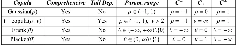
values from -1 to 1. Thus, it is desirable to use comprehensive copulas in modelling dependence of compet-ing causes of death. Applycompet-ing this criterion, we have selected the four copulas, introduced in Section 3, whose basic properties are summarized in Table 1. Here C-, C¦ and C+ denote the lower

Fréchet-Hoef-fding bound, the product copula and the upper Fréchet-HoefFréchet-Hoef-fding bound respectively.

Table 1.Selected bivariate comprehensive copulas: main properties.

Copula Comprehencive Tail Dep. Param. range C- _C

¦ C+

GaussianHrL Yes No r œH-1, 1L r = -1 r =0 r =1

t-copulaHr,nL Yes Yes r œH-1, 1L, n >2 r = -1 n = ¶ r =1

FrankHqL Yes No q œH-¶,+¶L\80< q = -¶ q =0 q = +¶

PlacketHqL Yes No q œH0,¶L\81< q =0 q =1 q = +¶

As seen from Table 1, the selected copulas depend on one or two parameters, not related to the parameters of the marginal distributions. The copula parameters, need to be estimated, based on a set of N pairwise observations on the survival times T1 and T2. However, there is only one observable survival time, i.e., the

minHT1,T2L and it is impossible to estimate the copula parameters, and hence to identify the joint survival

function SHt1, ...,tmL, by simply knowing the net survival functions S'HjLHtL, j=1, ...,m. For further

The fact that estimation of the copula parameter(s) is not possible imposes the necessity of considering them as free parameters. They could be set according to a priori available (medical) information, about the degree of pairwise dependence between the two competing risks, expressed through Kendall's t and/or Spearman's

rS. In what follows, we have set the copula parameters equal to fixed values, covering the whole range of

possible values of t and rS. Here, we provide a more detailed discussion on how this is done for the

exam-ple of the Gaussian copula case as an illustration.

As pointed out in Section 3.2, R12 can be expressed through the Kendall's tHT1,T2L, as given by (13), which

in this case is a free parameter, and hence, the dependence structure will have to be studied for different, fixed values of tHT1,T2L within the open interval H-1, 1L. Let us note that tHT1,T2L can not take the

bound-ary values -1 and 1, since in this case, the copula in (8) is not differentiable. Obviously, by fixing tHT1,T2L

we assume a certain degree of association (correlation) of the two r.v.s, T1 and T2, as given in terms of the

Kendall's t. This means that, when constructing the joint survival function of T1 and T2, we assume a

certain degree of dependence between the two causes of death, which we believe is realistic to admit. Thus, if tHT1,T2L=0.99, we assume a strong positive correlation between the two causes of death. This would

mean that, removal of one of the causes from our model will not significantly affect, i.e. improve the overall survival, since, due to their positive correlation the remaining cause will operate similarly as the removed one. If tHT1,T2L=0 then we are in the usual independence assumption. In the other extreme,

tHT1,T2L= -0.99 would mean that removal of one of the causes will significantly affect the overall

sur-vival, since due to the negative correlation, we assume that the remaining cause has an opposite effect on mortality to the removed one, and hence can not compensate for its removal.

All of the considerations made here for the two dimensional case carry over to the multivariate case, noting however, that in this case there is not a unique definition of an association measure, equivalent to Kendall's

t or Spearman's rS. One has to bear in mind, of course, that assumptions have to be made about all pairwise

coefficients tHTi,TjL, i, j=1, ...,m, i∫j which, for large values of m, will require careful consideration

(for m=2 one numerical value for t would need to be specified, but for m=3, 4, 5 and 6 one would need to specify correspondingly 3, 6, 10 and 15 entries for the corresponding correlation matrix R). So, one can conclude that the best approach to defining the values of t is to set them, based on medical or expert knowledge about the level of pairwise dependence between diseases. Obviously, some of the diseases may be expected to be mutually pairwise independent so, the corresponding t values can be set equal to zero.

Let us note that, in order to model extreme positive and negative dependence, i.e., when t takes values 1 and -1, it is more convenient to use the Frank copula.

4.2 Estimating and extrapolating the crude survival functions

As noted in Section 2, it is possible to estimate the crude survival functions, based on an appropriate m

dimensional set of cause specific, mortality data. If the data for each cause have already been smoothed they may then be directly interpolated, using spline interpolation or another alternative approximation method (see e.g., Dellaportas et. al, 2001). Here, we propose using the 'data averaging' optimal spline interpolation method described by De Boor (2001). Applying this method, m spline models may be fitted to the sets of observed values for the m crude survival functions and smooth estimates of the crude survival functions,

SHjL_{HtL j=1, ...,m, could then be obtained.}

of one or more causes of death. There have been several approaches to extending life tables beyond an upper age limit, such as the old-age mortality standard, developed by Himes, Preston and Condran (1994), the old age part of the Heligman-Pollard mortality model (see Heligman-Pollard, 1980) and also the Coale-Kisker method of closure of mortality tables (see Coale and Kisker, 1990, developed from a previous paper by Coale and Guo, 1989, and a recent investigation by Renshaw and Haberman, 2003). For a more detailed account on these methods and their application we refer to Buettner (2004). Here, we have applied a differ-ent approach (described in the Appendix), based on an appropriate extrapolation of the spline interpolants, produced by the 'data averaging' method. As will be seen from our numerical results (see Section 7), and based on our experience of a number of examples, this method produces reasonable extrapolations of the mortality experience up to the oldest ages, in the range 100-120.

If the mortality data have not been smoothed, a (spline) smoothing method may be applied to the raw data. A good candidate for the purpose is the method of constructing 'geometrically designed' free-knot splines, called GeD splines, which is automatic and does not require any knowledge of the number of knots and their locations (see Kaishev, Dimitrova, Haberman and Verrall, 2004).

5. Evaluating the net and overall survival functions

Having fixed the copula function, CHu1, ...,umL, one may use (8) and evaluate the joint survival function

(14)

SHt1, ...,tmL=CHS'H1LHt1L, ...,S'HmLHtmLL

if the net survival functions S'HjL_{HtjL, j=1, ...,m were known. In order to find them, we may use the} relationship between S'HjL_{HtL and the crude survival functions, S}HjL_{HtL, j=1, ...,m given by Heckman and} Honore (1989) and also by Carriere (1994). Thus, under the assumption of differentiability of CHu1, ...,umL

with respect to ujœH0, 1L and of S'HjLHtjL with respect to tj>0, fort>0, the following system of

differen-tial equations holds

(15)

d

ÅÅÅÅÅÅÅ_{d t} SH1L_HtL=C1HS'H1L_{HtL, ...,S}'HmL_{HtLLµÅÅÅÅÅÅÅ}d d t S'H1LHtL d

ÅÅÅÅÅÅÅ_{d t} SH2L_HtL=C

2HS'H1LHtL, ...,S'HmLHtLLµÅÅÅÅÅÅÅ_{d t}d S'H2LHtL ª

d

ÅÅÅÅÅÅÅ_{d t} SHmL_HtL=C

mHS'H1LHtL, ...,S'HmLHtLLµÅÅÅÅÅÅÅ_{d t}d S'HmLHtL,

where

CjHu1, ...,umL

=

It is important to note that (15) is a system of nonlinear, differential equations which may be solved with respect to the net survival functions S'HjL_{HtL, once we have specified the type of copula function, and given} estimates of the crude survival functions SHjL_{HtL, j=1, ...,m in a suitable functional form, which can then} be substituted into the left-hand side of (15). Then, in order to obtain the net survival functions S'HjL_{HtL, we} need to find an efficient numerical method of solving the system (15). Once the net survival functions are obtained, we may substitute them into the copula on the right-hand side of (14) and evaluate the joint survival function, and in particular the overall survival function HtLªSHt, ...,tL, which is of major interest in our investigation.

The derivatives with respect to time of the crude and net survival functions in (15) are actually the crude and net probability density functions of the r.v.s T1,T2, ...,Tm. We will denote these densities as f HjLHtL and

In order to solve the system (15) numerically, one can rewrite it as a system of difference equations, assum-ing that the time variable t¥0 takes integer values, (i.e., integral age values) k=0, 1, 2, .... This has been the approach taken by Carriere (1994). Its disadvantage is that the net survival functions S'HjL_HtL,

j=1, ...,m are obtained only for integral ages. Here, we have used the Mathematica built-in function

NDSolve, which solves numerically systems of differential equations and produces solutions, S'HjL_HtL,

j=1, ...,m, for any t>0.

Let us also note that we have used equality (5) as a check on the solution of (15). For this purpose, we can apply (14) to express the overall survival function on the left-hand side of (5) as

(16)

CHS'H1L_{HtL, ...,S}'HmL_{HtLL =S}H1L_HtL+....+SHmL_{HtL, 0§t§120.}

Equality (16) implies that if, for any fixed t, we substitute the values of the net survival functions

S'H1L_{HtL, ...,S}'HmL_{HtL, obtained as a solution of (15), in the copula function, its value must be equal to the sum} of the m crude survival functions, evaluated at t.

6. Partial and complete disease elimination

In order to study the effect of partial and complete disease elimination, we have adopted the following approach. Let us recall that, in our model, we have assumed that T1,T2, ...,Tm are the future lifetime spans

of a newborn individual, under the operation of m causes of death, i.e., all the survival functions, introduced up to now, refer to age zero. We will now need to adjust explicitly the adopted notation for the crude and net survival functions, by adding a 0 subscript, indicating age at birth, i.e., we will write S0HjLHtL, and S0'HjLHtL

instead of SHjL_{HtL and S}'HjL_{HtL, and also S}

xHjLHtL, and Sx'HjLHtL to denote the corresponding crude and net survival

functions for a life aged x. In order to illustrate the concept of partial and complete disease elimination, we will assume here that t takes integral values, i.e., tªk=1, 2, ...,120. Thus, we can express the net survival functions S₀'HjLHtL, j=1, ...,m, which we obtained as a solution of (15) as

(17)

S0'HjLHkL=S0'HjLH1LµS1'HjLH1Lµ∫µSk'-H1jLH1L .

Applying the well known relation Sx'HjLHkL=S0'HjLHx+kL ëS0'HjLHxL to the factors on the right-hand side of (17),

we obtain the convenient identity

(18)

S₀'HjLHkL=IS₀'HjLH1L ëS₀'HjLH0LMµIS₀'HjLH2L ëS₀'HjLH1LMµ∫µIS₀'HjLHkL ëS₀'HjLHk-1LM

Rewriting (18) in actuarial notation gives

(19)

S0'HjLHkL=p'0µp'1µ...µp'k-1=H1-q'0LµH1-q'1Lµ∫µH1-q'k-1L,

where, for simplicity, the dependence on the index j on the right-hand side has been suppressed. We now introduce the piecewise linear function qlHa,b;c,dL, with respect to l=0, 1, 2, ..., as

(20)

qlHa,b;c,dL= a, if lœ@0,cD

=a+

ÅÅÅÅÅÅÅÅÅÅ

=b, if lœ@d, 120L ,

We shall use qlHa,b;c,dL to modify the net survival function in (19), in order to be able to control the

degree of elimination of the j-th disease. Thus, if we denote by S₀''HjLHkL the modified net survival function and set q''l= H1- qlLq'l, l=0, 1, 2, ...,k-1, (19) can be rewritten as

S0''HjLHkL=H1-q''0LµH1-q''1Lµ∫µH1-q''k-1L.

By appropriately choosing particular values of the parameters a,b,c and d, for each age, the degree of elimination may be varied with the age l, with reasonable flexibility, from partial to complete elimination of the particular j-th cause of death. We may see how the modification of the net survival function (i.e., the degree of its elimination) will affect the overall survival function by substituting S₀''HjLHkL back into the copula, which defines the joint survival function in (14), i.e., the overall survival function becomes

HkLªSHk, ...,kL=CIS0'H1LHkL, ...,S0'Hj-1LHkL,S0''HjLHkL,S0'Hj+1LHkL, ...,S0'HmLHkLM

where k=0, 1, ..., 120. So, by varying the parameters a,b,cand d, one can adjust the degree of elimina-tion of the j-th cause of death at different ages and study its effect on HkL in the m-variate dependent multiple cause of death model. Let us note that the choice of a=b=1corresponds to qlª1, for

l=0, 1, 2, ....k-1 which leads to S0''HjLHkLª1, k=0, 1, 2, ..., which corresponds to complete elimination

of the j-th disease, since obviously, the overall survival function with j-th disease removed is

H-jLHkL=PrHT1>k, ...,Tj-1>k,Tj+1>k, ...,Tm>kL=

CIS0'H1LHkL, ...,S0'Hj-1LHkL, 1,S0'Hj+1LHkL, ...,S0'HmLHkLM.

An numerical implementation of complete and partial elimination is presented in Section 7.

7. Numerical results and conclusions

In this section, we will apply the methodology, described earlier, to a real data set, related to the US female general population, in which the data are grouped by causes of death, using "Table 10. Number of life table deaths from specific causes during age interval for the female population: United States, 1989-91" of the U.S. Decennial Life Tables for 1989-91 (see NCHS, 1999). For ease of presentation, we will consider the two dimensional and the multidimensional competing risk models separately.

7.1 Two causes of death

We consider here the simplest case of only two competing causes of death, one due to cancer, and a second one due to all other, non-cancer causes, pooled together. Thus, all the results of Sections 2-6 apply here for the case of m=2. Denote by Tc and To the lifetime random variables for the cancer and non-cancer causes

actual numbers, as well as the method and formulae, used to obtain the 'observed' and extrapolated values of the crude survival functions are given in the Appendix.

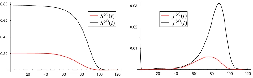
The fitted cubic spline curves SHcL_{HtL and S}HoL_{HtL, 0§t§120 and their derivatives are given in Figure 1. As} can be seen, the spline models of the two crude survival functions and the corresponding densities are smooth and posses very good visual quality.

20 40 60 80 100 120

0.20 0.40 0.60 0.80

SHoL_HtL

SHcL_HtL

20 40 60 80 100 120

0.01 0.02 0.03

fHoL_HtL

fHcL_HtL

Fig. 1. Interpolated crude survival functions (left panel) and their densities (right panel) for 'cancer' and 'other' causes of death.

Having estimated the crude survival functions SHcL_{HtL and S}HoL_{HtL, 0§t§120, we obtain the net survival} functions S'HcL_{HtL and S}'HoL_{HtL, 0§t§120, by solving the system (15), using the four copulas, specified in} Table 1. The solutions S'HcL_HtL,S'HoL_{HtL, 0§t§120, obtained from (15) have been checked, using equation} (16) for the case m=2. Since the solutions S'HoL_{HtL and S}'HcL_{HtL approach zero very closely in the age range} 100§t§120, solving (15) is much more difficult for 100§t§120 and the solution there may not possess the built-in Mathematica precision. Another important point is that the numerical solution of (15), S'HoL_HtL and S'HcL_{HtL, is influenced by the extrapolated sections of the crude survival functions not only for} 100§t§120 but within the entire age range 0§t§120. This in turn means that the results and conclu-sions with respect to survival under the dependent competing risk model, given later in this section, depend on the extrapolation that has been carried out.

7.1.1 The bivariate Gaussian copula case

The net survival functions, obtained as a solution of (15), using the Gaussian copula, CGa_Hu

1,u2L, with

values of r corresponding to five different values of Kendall's t are plotted in Fig. 2 (so that t =0.91 corresponds to r =0.99, t =0.35 corresponds to r =0.52 and so on). As explained in Section 4.1, the linear correlation r is considered as a free parameter, by means of which different degrees of association, between the cancer and non-cancer modes of death, are preassigned. Thus, the system (15) has been solved for values of r equal to -0.99, -0.52, 0.00, 0.52, 0.99 and the obtained net survival functions S'HoL_{HtL and}

20 40 60 80 100 120 0.2

0.4 0.6 0.8 1

S'HoL_HtL

0.91 0.35 0

-0.35

-0.91t

20 40 60 80 100 120

0.2 0.4 0.6 0.8 1

S'HcL_HtL

0.91 0.35 0

-0.35

-0.91t

Fig. 2. The net survival functions S'HoL_{HtL, 0§t§120 for 'other' (noncancer) cause (i.e. cancer removed)} -left panel and for 'cancer' (i.e. 'other' cause removed) - right panel.

As can be seen from the left panel of Fig. 2, removing cancer affects survival most significantly when Kendall's t = -0.91 (rS= -0.99), which corresponds to the case of extreme negative dependence. This

effect of rectangularization of the net (overall) survival function is seen even more clearly on the right panel of Fig. 2, where the 'other' cause of death has been removed. In addition, we note that in the case of negative dependence or even independence between Tc and To, the trend of the overall survival curves suggests that

the limiting age lies somewhere beyond 120 and it would not be natural to expect the old age survivors to die almost simultaneously at 120.

For the example of the bivariate Gaussian copula with Kendall's t = -0.91 (rS = -0.99), we will illustrate

how, not only a complete, but also a partial elimination of cancer, will affect the overall survival function

HtLªSHt,tL, 0§t§120. As described in Section 6, we apply the function qt, given by (20) to modify the

cancer net survival function S'HcL_{HtL. The results are illustrated in the right panel of Fig. 3, where SHt,tL,} 0§t§120, is evaluated and plotted for five different choices of the function qtHa,b;c,dL, plotted in the left

panel of Fig. 3. As can be seen from Fig. 3, for any fixed age t, the probability of overall survival increases if we vary qt from qtª0 (a=b=0) - the solid curve, corresponding to no elimination, through qtª0.5

(a=b=0.5) - the dot-dashed curve, corresponding to half elimination equally applied for 0<t<120, to

qtª0.9 (a=b=0.9) - the double dot-dashed curve, corresponding to almost complete cancer elimination.

qtH0.2, 0.8; 20, 65L represents respectively 20% cancer elimination for ages 0<t§20, linearly increasing

elimination from 20% up to 80% for 20<t§65 and 80% cancer elimination for 65<t<120. The remaining choice qtH0.8, 0.2; 20, 65L is similar but with the 20% and 80% parameters interchanged.

1 20 65 120

0.2 0.5 0.8 0.9

1 qt

1 20 65 120

0.2 0.5 0.8 0.9

1 SHt,tL

Fig. 3. The effect of different degree of partial elimination of cancer on the overall survival function

7.1.2 Sensitivity of the results with respect to choice of copula

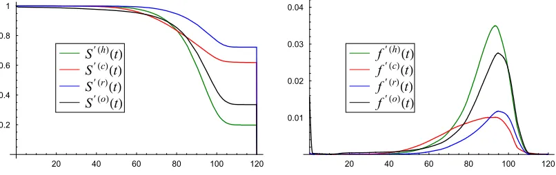
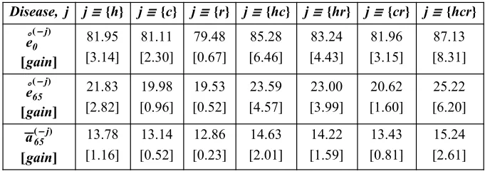
In this Section, we present a comparative study of the survival under the dependent competing risk model with respect to different choices of copula functions. For reasons stated in Section 4.1, we have performed the comparison by testing the proposed copula-based competing risk methodology with four different copulas, the Gaussian, the Student t-copula, the Frank and the Plackett copulas. For each copula we have used five different values of Kendall's t equal to -0.91, -0.35, 0.00, 0.35, 0.91. The results obtained show that the overall survival, given that cancer were eliminated as a cause of death, is most strongly affected by the choice of the copula in the case of extreme negative dependence, t = -0.91 and with the increase of t this effect decreases. The curves of the density f'HoL_{HtL, 0§t§120, for the four choices of} copulas, are plotted in Fig. 4 in the case of t = -0.35- left panel and t =0.35 - right panel.

20 40 60 80 100 120

0.01 0.02 0.03 0.04

f'HoLHtL,t =-0.35

Plackett Frank t-copula Gaussian

Copula

20 40 60 80 100 120

0.01 0.02 0.03 0.04

f'HoLHtL,t =0.35

Plackett Frank t-copula Gaussian

Copula

Fig. 4. The effect of the choice of copula on the overall survival density, f'HoL_{HtL, given cancer eliminated.} Although in the model presented here, it is more reasonable to look at the overall survival function HtL, 0§t§120, the joint survival function of Tc and To, SHt1,t2L=PrHTc>t1,To>t2L, 0§tj§120, j=1, 2, is

also of interest. However, since either one of the causes leads to death, and the other lifetime remains latent, probabilistic inference related to the joint distribution of Tc and To is somewhat artificial. Nevertheless, it is

instructive and in Fig. 5-8 we have illustrated the joint density of Tc and To in case of the bivariate

Gauss-ian, Student t-, Frank and Plackett copulas. For any bivariate copula, the joint density of Tc and To can be

calculated from (14) as

(21)

∑2

ÅÅÅÅÅÅÅÅÅÅÅÅÅÅÅ_{∑t1 ∑t2} SHt1,t2L=cHS'HcLHt1L,S'HoLHt2LLµf'HcLHt1Lµf'HoLHt2L.

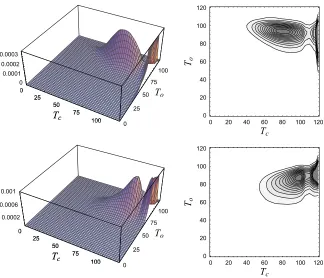
In the upper panels of Fig. 5-8, negative dependence between Tc and To has been modeled with

tHT1,T2L= -0.35, and in the lower panels, the modeled dependence is positive with tHT1,T2L=0.35. The

mass of the distribution is oriented in such a way that, under negative dependence, as seen from the upper panels of Fig. 5-8, higher values of To are more likely to occur jointly with smaller values of Tc. Under

positive dependence, as seen from the lower panels, jointly increasing values of the lifetimes Tc and To are

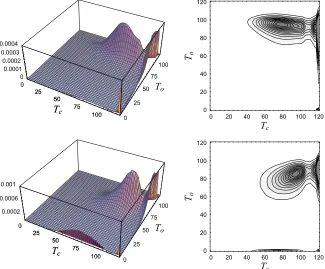
likely to occur. This is valid, regardless of what copula has been used, as can be seen from Fig. 5-8. There are, of course, some copula specific differences in the joint density functions, as is natural to expect in view of (21). For example, in the case of Student t-copula, there are probability masses in the corners inherited from the density of the copula itself (Fig. 6). In other cases, the joint density is significantly influenced by the (marginal) net survival functions, which cause probability masses to occur along the borders Tc=0

and/or To=0, as e.g., in the case of Frank copula (Fig. 7). Another, obvious characteristic of the joint

density function is that for t = -0.35 it has one mode approximately around To=90, Tc=80 and for

0 25 50 75 100 Tc 0 25 50 75 100 To 0.0002 0.0006 0.001 0 25 50 75 100

Tc _{0 20 40 60 80 100 120}

Tc 0 20 40 60 80 100 120 To 0 25 50 75 100 Tc 0 25 50 75 100 To 0 0.0001 0.0002 0.0003 0 25 50 75 100 Tc

0 20 40 60 80 100 120

Tc 0 20 40 60 80 100 120 To

Fig. 5. A 3D plot and a contour plot of the joint density of Tc and To, expressed through the Gaussian

copula for Kendall's t = -0.35 (upper panel) and t =0.35 (lower panel).

0 25 50 75 100 Tc 0 25 50 75 100 To 0 0.0005 0.001 0.0015 0 25 50 75 100 Tc

0 20 40 60 80 100 120

Tc 0 20 40 60 80 100 120 To 0 25 50 75 100 Tc 0 25 50 75 100 To 0 0.0001 0.0002 0.0003 0 25 50 75 100 Tc

0 20 40 60 80 100 120

Tc 0 20 40 60 80 100 120 To

Fig. 6. A 3D plot and a contour plot of the joint density of Tc and To, expressed through the t-copula for

0 25 50 75 100 Tc 0 25 50 75 100 To 0.0002 0.0006 0.001 0 25 50 75 100

Tc _{0 20 40 60 80 100 120}

Tc 0 20 40 60 80 100 120 To 0 25 50 75 100 Tc 0 25 50 75 100 To 0 0.0005 0.001 0.0015 0.002 0 25 50 75 100 Tc

0 20 40 60 80 100 120

Tc 0 20 40 60 80 100 120 To

Fig. 7. A 3D plot and a contour plot of the joint density of Tc and To, expressed through the Frank copula

for Kendall's t = -0.35 (upper panel) and t =0.35 (lower panel).

0 25 50 75 100 Tc 0 25 50 75 100 To 0.0002 0.0006 0.001 0 25 50 75 100

Tc _{0 20 40 60 80 100 120}

Tc 0 20 40 60 80 100 120 To 0 25 50 75 100 Tc 0 25 50 75 100 To 0 0.0001 0.0002 0.0003 0.0004 0 25 50 75 100 Tc

0 20 40 60 80 100 120

Tc 0 20 40 60 80 100 120 To

Fig. 8. A 3D plot and a contour plot of the joint density of Tc and To, expressed through the Plackett copula