1
The added value from a general equilibrium analysis of increased efficiency
in household energy use
Patrizio Lecca1, Peter G. McGregor1, J. Kim Swales1 and Karen Turner2,a
1. Fraser of Allander Institute, Department of Economics and Strathclyde International
Public Policy Institute, University of Strathclyde
2. Centre for Energy, Resource and Environmental Studies and Department of Accounting,
Economics and Finance, School of Management and Languages, Heriot Watt University.
a. Corresponding author: [email protected].
Acknowledgments
The authors gratefully acknowledge the financial support of the ESRC through a First Grants
project (ESRC ref: RES-061-25-0010), the EPSRC’s Highly Distributed Energy Futures
Consortium (EPSRC ref: EP/G031681/1)and funding from the Scottish Government through
2
The added value from a general equilibrium analysis of increased efficiency
in household energy use
Abstract
This paper investigates the economic impact of a 5% improvement in UK household energy
efficiency, focussing specifically on total energy rebound effects. The impact is measured
through simulations using models that have increasing degrees of endogeneity but are
calibrated on a common data set, moving from a basic partial equilibrium approach to a fully
specified general equilibrium treatment. The size of the rebound effect is shown to depend on
changes in household income, aggregate economic activity and relative prices that can only
be captured through a general equilibrium model.
Keywords: Energy efficiency; indirect rebound effects; economy-wide rebound effects; household energy consumption; CGE models.
3 1. Introduction
There has been extensive investigation of the economy-wide rebound effects resulting from
energy efficiency improvements in production. This analysis often uses a computable general
equilibrium (CGE) modelling approach (see Dimitropoulos, 2007; Sorrell, 2007; and Turner
2013for a review). However, very few studies have attempted to measure the economy-wide
impacts of energy efficiency improvements in the household sector. Following the work of
Khazzoom (1980, 1987) there have been a numbers of partial equilibrium studies (Dubin et
al. 1986; Frondel et al. 2008; Greene et al. 1999; Klein, 1985 and 1987; Nadel, 1993;
Schwartz and Taylor, 1995; West, 2004). Further, Greening et al.(2000) gives a detailed and
extensive summary of the extent of rebound on household consumption of different types of
energy services. These studies assume that there are no changes in prices or nominal incomes
following the efficiency improvement, and that the impacts are limited to the direct market for
household energy use. This approach gives an extreme partial equilibrium figure, which is
generally known as the direct rebound effect.
To our knowledge, Dufournaud et al. (1994) is the only study that investigates full general
equilibrium economy-wide rebound effects from increased energy efficiency in the household
sector. It examines the impacts of increasing efficiency in domestic wood stoves in Sudan.
Druckman et al. (2011), Freire-Gonzalez (2011) and Thomas and Azevedo (2013a; 2013b)
use a fixed price input-output model to consider indirect rebound effects resulting from
household income freed up by energy efficiency improvements and spent on non-energy
commodities. This work includes changes in energy use in production, as well as household
consumption. However, we still treat this as a partial equilibrium approach as it fails to
4
The aim of the present paper is to identify the added value from using general equilibrium
techniques to consider the economy-wide impacts of increased efficiency in household energy
use. We take as an illustrative case the effect of a 5% improvement in UK household energy
efficiency. The subsequent impact on energy use is measured through simulations employing
models that have increasing degrees of endogeneity but are all calibrated on a common data
set. That is to say, we calculate rebound effects for models that progress from the most basic
partial equilibrium approach to a fully specified general equilibrium treatment.
2 Rebound Effects
We categorise an increase in household energy efficiency as being a change in household
“technology” that increases the energy services generated by each unit of physical energy
consumed. An alternative way of expressing this is that the energy value in efficiency units
has risen.1 This implies that the original level of household utility can be achieved through the
consumption of the original levels of other household goods and services, but with a lower
consumption of energy.2
We define the rebound effect as a measure of the difference between the proportionate change
in the actual energy use and the proportionate change in energy efficiency. This difference is
primarily driven by the fact that, ceteris paribus, an increase in the efficiency in a particular
energy use reduces the price of energy in that use, measured in efficiency units. This
reduction then leads consumers to substitute energy, in efficiency units, for other goods and
services implying that the proportionate reduction in energy use is typically less than the
1 We discuss in Section 3 how such efficiency improvements might come about.
2 We do not identify an improvement in household energy efficiency as simply a reduction in the direct energy
5
proportionate improvement in energy efficiency.3 This is the rebound effect. Moreover, in
principle, energy use can actually rise in these circumstances, if its use is sufficiently price
sensitive. This is known as backfire (Khazzoom, 1980 and 1987).
In the case under consideration here, for a proportionate improvement in household energy
use of γ, rebound in the household consumption of energy, RC, can be calculated as:
1 C 100
C E R
(1)
where EC is the proportionate change in energy use in household consumption, which may be
positive or negative.
We are also interested in the economy-wide rebound of household energy efficiency
improvements: that is to say, the impact on energy use in the economy as a whole, both in
consumption and production.4 The total rebound formulation used in this case, RT, is given as:
1 T 100
T E R
(2)
where α is the initial share of household energy consumption in total energy use. The term
T
E
can be expressed as:
C P C
T T P
C C C
E E E
E E E
E E E
(3)
3
The distinction between energy quantities and prices measured in natural and efficiency units is important in explaining how the rebound effect operates. However, in the present paper, unless we explicitly state otherwise, energy is being measured in natural units.
4 Our interest here is limited to the rebound effect within the target economy, so that we abstract from potential
6
where Δ represents absolute change and the P subscript indicates production. Substituting
equations (1) and (3) into equation (2) gives:
100
P
T C
C
E
R R
E
(4)
This shows that the total rebound will be higher (lower) than the consumption rebound if the
energy use in production increases (decreases) as a result of energy efficiency improvements
in consumption.
3. Data and elasticity of substitution of energy use in consumption
In this paper we identify the additional precision achieved through moving from a partial to a
general equilibrium analysis of the rebound effects. We consider the specific case of energy
efficiency improvements in household consumption.5 We quantify the rebound effect through
simulation using a given data set which provides common structural characteristics across all
the models. Specifically we use a specially constructed UK symmetric industry-by-industry
Input-Output (IO) table based on the published 2004 UK Supply and Use accounts.6 Import
data in Input-Output format were provided by colleagues at the Stockholm Environment
Institute. The Input-Output accounts are aggregated to identify 21 economic activities
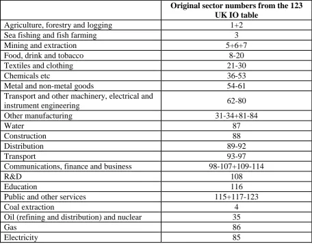
(commodities/sectors). Table 1 gives the sectoral disaggregation, separately identifying the
four energy sectors; coal, oil, gas and electricity.
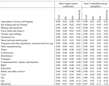
Table 2 identifies the energy input requirement for each of the production sectors and the
energy-output multiplier effects expressed in monetary terms. That is to say, for each sector
we measure the direct and indirect increase in the value of output in energy industries
5
We increase household efficiency in the use of all sources of energy: coal, oil, gas and electricity.
6
7
generated by a unit increase in the final demand for that sector. The energy requirements are
represented by the appropriate direct Input-Output coefficients (the A matrix entries) while
the energy-output multipliers are the corresponding entries in the Type I Leontief inverse,
[1-A]-1 inverse matrix. To calibrate the Computable General Equilibrium model, the
conventional Input-Output accounts are augmented with all other transfer payments to form
the 2004 UK Social Accounting Matrix.7 In all the analysis we use a single initial household
consumption vector given in UK 2004 Input-Output accounts.
A key parameter that drives rebound analysis is the elasticity of substitution between
aggregate energy and non-energy goods and services in the household’s utility function. In
each of the models we use, household utility, C, in any period is given by:
1 1 1(1 )
E E
C C
C E NE
(5)
NEC is the consumption of non-energy commodities, ε is the elasticity of substitution between
energy and non-energy commodities in consumption and E(0,1) is the share parameter.
We estimate the value of the elasticity of substitution using UK household consumption data
from 1989 to 2008 employing the conventional generalized maximum entropy (GME) method
(Golan et al. 1996).8 Details of the estimation procedure are reported in Lecca et al (2011,
2013b). The short- and long-run elasticities of substitution are estimated as 0.35 and 0.61
respectively. Our elasticity estimates are broadly in line with previous empirical evidence for
UK households (e.g. Baker and Blundell, 1991 and Baker et al. 1989).9
7 For more information on Input-Output accounts and Social Accounting Matrices see Miller and Blair (2009). 8
The value of the elasticity of substitution is likely to vary across types of energy services, such as personal transportation, residential space heating, etc. However, at this stage, for pedagogic reasons, we impose a common value across all household consumption energy uses.
9
8
We have estimated the substitution elasticities by observing the reaction of household energy
consumption to changes in energy price. However, the question arises as to whether the same
substitution elasticities are appropriate where efficiency improvements reduce the price of
energy, measured in efficiency units? The answer might lie in the nature of the efficiency
improvement. We see no reason not to use the run elasticity of substitution where
long-run simulations are performed. However, for short-long-run simulations it might be appropriate , in
some circumstances, to use the long-run elasticity value.
The short-run adjustment in household consumption of energy in response to a change in
energy prices might be lower than the long-run value for two different reasons. First, there
might simply be be a degree of inertia in the consumption response. However, a second
reason might be that a full adjustment to the new energy price requires an investment in
consumer durable goods, which only occurs in the long run.If the difference between the short
and long-run elasticities is primarily due to this second reason, and household energy
efficiency improvements are embedded in the design of consumer durables, it is appropriate
to use long-run substitution elasticities, even for short-run simulations. This is because to
access the efficiency improvement at all requires adjustment to the household capital stock
which is essentially a long-run adjustment.
4. A partial equilibrium framework
In our partial equilibrium analysis, we assume that the prices of all commodities and services,
including energy prices, are fixed and that there is no change in household nominal income.
This is the impact that would be appropriate for analysing the decision by a single household
9
improvement in energy efficiency in consumption, we are also interested in the subsequent
impact on energy use in production too. This can be achieved, whilst still maintaining the
partial equilibrium assumptions of fixed prices and household income, through the application
of conventional Type I Input-Output analysis.
4.1 Household energy use
To determine the level of rebound in household energy use, first we need to derive the
elasticity of demand, η, from the elasticity of substitution, ε. This is given as:
( 1)
(6)
where λ is the share of energy in household expenditure (Gørtz, 1977). From the UK 2004
Input Output accounts, 3% of household consumption is spent on energy so that λ = 0.03.
Given elasticities of substitution reported in Section 3, the short- and long-run energy price
elasticities calculated using equation (6) equal 0.37 and 0.62. Note that the long-run
elasticity is consistent with estimates elsewhere in the literature for transport and
non-transport related household activities (Fouquet, 2012; Fouquet and Pearson, 2012).
With no change in the price of energy, a proportionate increase in efficiency in household
energy consumption, γ, generates an equal proportionate reduction in the price of energy to
consumers, measured in efficiency units. If the elasticity of demand for energy is η, where η
takes a positive sign, the proportionate change in consumer energy demand, measured in
efficiency units, ECF, is given as:
F C
E (7)
The proportionate change in consumer energy use, measured in natural units, is the
10
( 1)
C
E (8)
where 0and EC 0
.
Substituting expressions (6) and (8) into equation (1) produces:
100 100( ( 1) )
C
R (9)
Using the short- and long-run demand elasticities produces the short- and long-run household
consumption rebound values of 36.9% and 62.2%. These values are entered in the top row of
Table 3. Equation (9) calculates what is conventionally known as the direct rebound.10 These
figures lie within the range of available US and European estimates for specific household
energy uses (Freire-Gonzales, 2010; Greening et al., 2000). A comprehensive review of
empirical estimates of direct rebound effects is provided by Sorrell et al. (2009).
4.2 Total energy use
In the analysis reported in Section 4.1, the improvement in energy efficiency operates in a
manner that is observationally equivalent to a change in the representative household’s tastes,
with fixed nominal income and prices. Whilest household utility will rise, the economic
impact is reflected solely in consumption shifting.11 With rebound values less than 100% this
implies a fall in consumption expenditure on energy and an increase in the expenditure on all
other goods and services.
We can retain the partial equilibrium assumptions of fixed prices and household income but
incorporate the impact on total energy use by adopting a Type I Input-Output analysis (Miller
and Blair, 2009). In this approach, the impact on energy use in both household consumption
10 We consider the estimated elasticity of energy demand as a proxy of the direct rebound effects (Khazzoom,
1980). This is the easiest and more straightforward definition of direct rebound, though it has been criticized by Sorrell and Dimitropoulos (2008) as subject to bias.
11
11
and industrial production is identified and the relevant total rebound measure, as expressed in
equation (2), can be calculated. This captures the notion of energy being embodied in
consumption goods or services, in the form of the energy required, directly or indirectly, in
the production of these goods and services.
We introduce a shock in the Input-Output system by reducing household final consumption
expenditure on both UK and imported energy (coal, oil, gas and electricity). We
simultaneously increase household spending on other (non-energy) goods and services, using
the distribution of initial expenditure on domestic and imported non-energy goods and
services given in the Input-Output accounts. This method shares some characteristics with
Freire-Gonzalez (2011) and Thomas and Azevedo (2013a; 2013b) and extends Druckman et
al. (2011) by incorporating the impact on indirect rebound from the reduction in energy use
embodied in the reduction in domestic energy supply itself.
The change in household consumption expenditure on energy, ΔEC, is matched by an equal
and opposite change in non-energy household expenditure, ΔNEC, and is given as:
1 100
C
C C T
R
E NE X
(10)
where XT is total household expenditure. Using Type I Input-Output multipliers, the change in
total energy use, ΔET, equals:
(1 E) E
T C E C NE
E E m NE m
(11)
where mEE and mNEE are respectively the amounts of energy used domestically, directly or
indirectly, in the production of one unit of energy and one unit of non-energy household
consumption. Household energy use can be expressed either as the share, λ, of the total
12 T X E (12)
Combining equations (10), (11) and (12) produces:
1 (1 )
100
E C
T
R
E m
(13)
where mEmEEmNEE . Substituting equation (13) into equation (2) gives:
(1 E) 100 E
T C
R R m m (14)
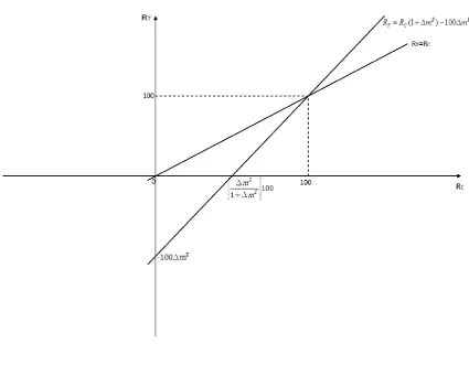
Equation (14) expresses the total partial equilibrium rebound, RT, as a function of the rebound
value in the household consumption of energy, RC, and the difference between the embodied
energy in the production of energy and non-energy goods and services, ΔmE. We expect the
production of energy to be relatively energy intensive, so that ΔmE > 0: this is certainly the
case in the UK Input-Output accounts. Combined with equation (14), this implies that the
relationship between the partial equilibrium total and household consumption rebound is
represented in Figure 1.12 As a benchmark, we also show in Figure 1 the locus of points where
RC =RT.
It is clear from Figure 1 that where there is backfire in the household consumption of energy,
so that RC > 100%, the partial equilibrium rebound value for total energy use is greater than
the value for household energy consumption. However, where RC < 100%, the total rebound
value is less than the corresponding household value. Further, there is a range of values for
RC, 0 100
1 E C E m R m
, for which the total partial equilibrium rebound value is negative.
12
13
This means that the proportionate total energy reduction is greater than the efficiency
improvement.
We can quantify the partial equilibrium total rebound generated by the consumption
expenditure shifting associated with the improvement in household energy efficiency. Note
that whilst we assume that the full adjustment of consumption expenditure to the change in
household energy efficiency might take some time, the IO method for identifying energy use
changes in production makes no such assumption. The passive supply implies that existing
capacity already exists to meet any adjustments in demand.
For the 36.9% household consumption rebound value estimated using the short-run elasticity
of substitution, the proportionate reduction in household consumer expenditure on energy,
,
C
E equals 3.16%. This corresponds to a 109355 TJ reduction in household energy use and to
a £752.57 million reallocation in UK household consumption across the seventeen non-energy
consumption sectors. The result is a fall in total energy demand of £1002 million (137363 TJ)
which corresponds to 1.44% of total UK energy use (across households and producers), so
that ĖT = - 1.44% . Given that γ = 5% and α, the share of household consumption in total
energy use, equals 0.344, the total rebound value (RT) takes a value of 16.0 %. The indirect
component of the rebound effect is therefore negative with a value of 20.9%. 13
Where the estimated long-run demand elasticity is used in the rebound calculations, there is a
larger household consumption rebound value. This implies a smaller reallocation of
household expenditure in favour of non-energy goods and services. In this case, ECindicates
a 0.87% fall in expenditure on energy, a reduction of 65509 TJ which equates to £450.9
million to be reallocated to non-energy household consumption. The total energy rebound, RT,
13
14
is 49.7%, with the impact of indirect expenditures, RT - RC, being to reduce the rebound by
12.54 percentage points. These figures for the partial equilibrium total rebound are entered
into the first row of Table 3.
Generally, there is an expectation that the total rebound will be bigger than the household
consumption value. However, as we have seen, this does not hold in partial equilibrium if
household rebound is less than 100%. The indirect component of the rebound in this case is
negative, putting downward pressure on the total rebound value. This effect will persist in a
general equilibrium approach, as long as the balance of consumer expenditure moves towards
non-energy commodities. However, the magnitude of this negative rebound component, being
driven by changes in the demand for intermediate inputs, will be influenced by endogenous
price, income and supply responses. For example, as demand for energy falls in the short run
as a result of the pure efficiency effect, the market price may decrease, stimulating the derived
demand for energy use in production. Similarly, the output of all commodities will be affected
through changes in competitiveness, further influencing the demand for energy as an
intermediate input. Finally, changes in domestic prices also impact the revenues of domestic
producers, leading to adjustments in capacity in the general equilibrium setting to which we
now turn our attention.
5. General equilibrium rebound effects – endogenous prices and incomes
The analysis in Section 4 holds prices and nominal household income fixed. In the analysis in
this section, we allow prices and incomes to vary in determining the rebound effect. These
effects are captured through the use of Computable General Equilibrium (CGE) modelling.
To identify the general equilibrium impacts, we use a variant of the UKENVI CGE modelling
15
calibrated on a UK Social Accounting Matrix (SAM) (Allan et al. 2007; Harrigan et al. 1991
and Turner, 2009).14 The core of the 2004 SAM is the 21 sector Input-Output table used in
Section 4. This is augmented with information on income transfers between aggregate agents.
These comprise the UK household, government and corporate sectors, plus two external
transactors, the rest of the UK (RUK) and the rest of the world (ROW). We introduce a
capital account that balances income and expenditures through which all capital formation is
funded, and two factor accounts for incomes from capital and labour where incomes are
initially channelled through the domestic agent accounts. Additional data used in the
construction of the SAM are drawn mainly from National Statistics (2004).
Simulations performed under Scenario 1 use the standard model, UKENVI, as employed in
Allan et al. (2007) and Turner (2009), augmented so that consumption and investment
decisions reflect inter-temporal optimization with perfect foresight (Lecca et al. 2013a). The
model is outlined in more detail in Appendix A and the full mathematical presentation of the
model can be found in the supplementary material accompanying this paper.
Under Scenario 2, the increased energy efficiency in household consumption is directly
reflected in real wage determination, given in equation (A.3) in Appendix A. This involves
modifying the consumer price index (cpi) so that the price of energy services is expressed in
efficiency units. . We can incorporate the efficiency change in the wage bargaining process by
simply adjusting the cpi by measuring the price of energy in efficiency units:
1
F E
E E
p
p p
for 0 (15)
so that
14 AMOS is an acronym for A micro-macro Model Of Scotland. Whilst AMOS was initially calibrated on
16 ( NE, EF)
cpi cpi p p (16)
where pNE is the price of non-energy goods and services, and pE and pEF are the price of
energy measured in natural and efficiency units. This means that with constant energy prices
in natural units, pE, an improvement in energy efficiency reduces the price of energy in terms
of efficiency units, pEF. In this scenario, this reduces the cpi which has a direct effect on the
nominal wage rate.
The model calibration process assumes the economy to be initially in steady state equilibrium.
As in the partial equilibrium simulations, we introduce a costless and permanent 5% step
increase in the efficiency with which energy is used in household consumption. We report
results for two conceptual time periods, the short and the long run, together with
period-by-period impacts for some simulations. The short run corresponds to the first period-by-period of the
simulation, where the capital stock is fixed, both in its total and its sectoral composition, at
the base period values. However, from period two onwards, capital stock adjusts through
investment and depreciation. In the long run, the state variables of the model are subject to
transversality conditions, so as to obtain a new steady-state.
As discussed in Section 3, when the analysis applies to the long run, we always use the
long-run elasticity of substitution. However, in the short long-run, we perform simulations using both
the short-run and long-run substitution elasticities. Recall that the long-run elasticity values
might be more appropriate, even in short-run simulations, if energy efficiency is embodied in
the design of consumer durables.
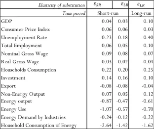
Table 4 shows the short and long-run impact of the improved household energy efficiency on
17
label this Scenario 1. We report the results as percentage changes from the base year values.
In Scenario 2, the model is adjusted, as shown in in equation (15) and (16), so that the cpi
incorporates the price of energy in efficiency, rather than natural, units. The results from this
simulation are reported in Table 5.
5.1 Scenario 1: The standard model
The Scenario 1 results are given in Table 4. In the short run, simulations using the short-run
elasticity of substitution report a 2.64% reduction in household energy consumption. The
switch in household expenditure towards non-energy consumption has a small expansionary
impact on the economy: total output, consumption and investment increase by 0.04%, 0.22%
and 0.14% respectively.15 There is a corresponding stimulus to labour demand, lowering the
unemployment rate by 0.23% and increasing the real wage by 0.03%.
The fall in energy demand from households is accompanied by a 0.24% fall from industry
because of the relative energy intensity of the production of energy itself. This is the same
source of negative total rebound pressure identified in Section 4. Total energy use and output
fall by 1.07% and 0.87% respectively. However, energy prices are now endogenous and fall
in the short run, shown in Figure 2. This means that the decline in domestic energy use is
partly offset by some substitution towards energy in production and changes in output driven
by adjustments in exports and import substitution. The short-run increase in exports produced
by the increase in competitiveness is illustrated in Figure 3. These price reductions are caused
by the short-run emergence of overcapacity in those sectors following the efficiency
improvement.
15 The household consumption value is the change in real household consumption. This implies that the increase
18
The second column of Table 4 reports the short-run impacts where the long-run elasticity of
substitution between energy and non-energy goods and services is imposed. Note that in this
case there is a smaller reduction in household consumption of energy of 1.42%. This means
that there is less expenditure switching, which has two general implications. The first is that
the expansionary impacts, whilst still present, are all slightly smaller than where the short-run
elasticity is used. This is because non-energy expenditure has a greater impact on the UK
economy than the same amount of expenditure on energy. The second is that the total
reduction in energy use is also lower, at 0.57%.
In the long-run results, shown in the third column in Table 4, household consumption of
energy, energy demand by industry, total energy use and total energy output all remain below
their base-year values. However, there is a 0.10% increase in GDP and similar increases in
total employment and investment. The expansion in the long run is greater than in the short
run as the ability to adjust capacity allows a greater response to the net positive demand
stimulus. Because the labour force is assumed to be fixed, there is a fall in the unemployment
rate generating an increase in the real wage which, in turn, puts upward pressure on all
commodity prices and reduces competitiveness. This is shown in Figures 2 and 4.
Figure 4 reports the percentage change in sector prices relative to the base year level for the
whole period of adjustment, using the long-run elasticity of substitution value in each time
period. The demand shock generates short-run shifts in prices which reflect the change in
household demand. There are short-run price reductions in coal, gas and electricity but
corresponding price increases in all other sectors. Over time, the adjustment of capacity leads
to small increases in prices in all sectors. The long-run price behaviour differs from that
19
the economy. For improvements in energy efficiency in production, economic activity is
stimulated through downward pressure on prices. This includes the price of energy output
itself since the energy supply sector is typically energy intensive.
While the increase in total investment in Scenario 1 means that there is an increase in capital
stock over time in non-energy sectors, decreased output leads to a contraction in capacity in
energy sectors. The trigger for this disinvestment is the fall in the shadow price of capital
caused by the initial contraction in demand for energy sector outputs. Energy firms’ profit
expectations therefore fall. This is reflected in Figure 5, where we plot the shadow price of
capital and the replacement cost of capital for the energy sectors. In each of these sectors, the
shadow price of capital is below the replacement cost of capital over the entire adjustment
path, implying that Tobin’s q < 1 in these sectors. Ultimately, there is complete adjustment
where the capital stock reaches the steady-state equilibrium. After the initial fall, the price of
energy rises over time, allowing the shadow price of capital to converge on the replacement
cost of capital, so that Tobin’s q asymptotically approaches unity.
Again, using equations (1) and (2) and the household and total energy change figures
identified in this section we can calculate the household and total energy rebound effects.
These are reported in rows 2 and 3 of Table 3. In the short-run simulations the rebound values
for household energy use are 47.3%, using the short-run elasticity of substitution, and 71.6%
for the long-run value. The corresponding short-run general equilibrium total rebound values
using the short- and long-run substitution elasticities are 38.5% and 67.1% respectively. For
the long-run values, which always use the long-run substitution elasticity, the household and
total rebound values are 67.6% and 59.3%.
20
In Scenario 1, the increase in energy efficiency in the household sector acts in a way that is
observationally equivalent to a change in tastes. This is because, as shown in equation (14), in
the calculation of the real wage the consumer price index, cpi, combines the price of
non-energy and non-energy commodities measured in natural units. However, it might be more
appropriate in defining the cpi to measure the composite energy price in efficiency units. This
implies that the cpi should be calculated as in equations (15) and (16). With this approach, in
so far as improvements in energy efficiency reduce the energy price (measured in efficiency
units), this will be translated into a fall in the cpi, which will put downward pressure on the
nominal wage and serve as a source of improved competitiveness.
Scenario 2 repeats the simulation of a 5% step increase in energy efficiency in household
consumption. All aspects of the simulations are exactly the same as those reported for
Scenario 1 in Section 5.1, apart from the difference in the calculation of the cpi. The
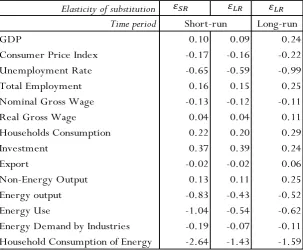
percentage changes in key economic variables are reported in Table 5 and the corresponding
rebound values in Table 6. The changes in the prices for individual commodities over time are
given in Figure 6.
In the standard case reported as Scenario 1, both the cpi and the nominal wage rise and are
maintained above their base year values in the long run. However, in Scenario 2, these results
are reversed. In the short run, both the short or long-run substitution elasticity simulations
produce a fall in the nominal wage of 0.13% and 0.12% respectively. The fall in the nominal
wage in the long run is 0.11%. As shown in Figure 6, this reduction in labour costs generates
a fall in the price of output in all production sectors. The resulting stimulus to competitiveness
has an expansionary effect that offsets the impact on aggregate demand of a lower nominal
21
than Scenario 1. All these aggregate activity variables increase in the long run by around
0.25%.
The reduction in energy use is always bigger in Simulation 1 than in the corresponding result
under Simulation 2. That is to say, the bigger stimulus to the economy under Simulation 2
reduces the energy saving. However, the additional impact on energy use and the associate
rebound effects are small. Even in the long run, where the relative expansionary effect of the
increased energy efficiency is greatest, the total energy rebound for Scenario 2 is 54.3%,
against the Scenario 1 figure of 48.5 %.
6. The added value from a general equilibrium analysis
In comparing the general and partial equilibrium analysis, and therefore the added value from
a general equilibrium approach, we begin by considering the rebound values for the
simulations in Scenario 1, reported in Table 3. These results reveal that the same basic data
can generate a wide range of possible rebound figures, which depend upon the narrowness of
the focus of the analysis, the value of key parameters, the time scale and whether a partial or
general equilibrium approach is adopted.
The first row in Table 3 gives the partial equilibrium values. Recall that these apply to the
rebound on an individual household’s energy consumption if that household alone
experienced the improved energy efficiency, with money income and energy prices
unchanged. First, focus on the household energy rebound, which solely concerns the direct
energy use by households. Clearly general equilibrium effects are not required in order to get
substantial rebound values. Moreover, comparing the results with short and long-run values,
22
consumption, that is, the more flexible consumption is in accommodating the efficiency gains,
the greater the rebound will be. Second, the total rebound values are less than the household
consumption values. This reflects the shift of household expenditure away from the
intermediate demand energy intensive energy sectors towards less energy intensive
commodities and services, as argued in Section 4.2. Moreover, the difference between the
total and household consumption rebound values narrows as the household consumption
value increases, as shown in Figure 1.
A general equilibrium analysis involves incorporating the effect on energy use of endogenous
changes in prices, wages and incomes. Consider first the short-run Scenario 1 values given in
row two in Table 3. The effect of the change in household income and prices over this time
interval increases the household rebound values by around 10 percentage points. The increase
is slightly greater when using the short-, as against long-run substitution elasticity. Household
income increases in real term by around 0.06% for both short- and long-run substitution
elasticities. For an income elasticity equal to one, as imposed in this model, we should expect
a similar percentage increase in household energy consumption (although the linearity
assumption between income and consumption does not strictly hold here given the perfect
foresight of households). As a result, in these simulations changes in endogenous household
income increase the general equilibrium rebound values by around 1.2 percentage points. The
relative price changes, shown in Figure 4, generate the remaining, larger, household rebound
effects of around 9 percentage points. The short run significant falls in energy prices in
natural units, as a result of temporary excess capacity, leads to the substitution of energy for
other commodities in the household budget.
For total energy use, the gap between the partial and general equilibrium short-run rebound
23
higher under general equilibrium than partial equilibrium. Again the additional rebound is
slightly bigger for the short-run substitution elasticities. The difference between the partial
and general equilibrium total rebound values include changes already identified as
contributing to household rebound. These stand at just over 10 percentage points. However,
there are three additional factors operating on total energy use in general equilibrium and they
all increase the total rebound figure.
First, the negative impact on rebound through the different energy intensities of the
intermediate inputs in energy and non-energy sectors is reduced following the increased
rebound in household consumption as indicated in Figure 1. This makes up 3 percentage
points. The remaining 7 percentage point difference comes from additional relative price
effects on intermediate energy demand. These comprise the substitution of energy for
non-energy commodities as intermediate inputs together with the fall in exports and increased
import penetration in non-energy sectors, and the rising exports and import substitution in
energy sectors. The difference between the general and partial equilibrium short-run total
energy rebound values is therefore driven primarily by endogenous relative price, rather than
income, effects.
The long-run general equilibrium rebound figures for Scenario 1 are shown in row 3 of Table
4. For both the household and total energy rebound, the long-run general equilibrium value
lies between the corresponding partial equilibrium and short-run general equilibrium figures.
The long-run general equilibrium simulations generate larger positive changes in household
income and GDP than the partial equilibrium or short-run general equilibrium values.16
However, over the long run, capacity adjustments reduce the changes in commodity prices,
16 Change in real income is around 0.10% from base year value. Generally the long-run change in income should
24
which are ultimately only driven by the impact of the higher nominal wage across different
sectors. This means that the substitution and competitiveness effects that increase the rebound
effects under short-run general equilibrium are much reduced in the long run. However, a key
point to note is that there is a mix of positive and negative pressure impacting the general
equilibrium rebound results in both the short-run and the long-run.
In Scenario 2, the improvement in household efficiency in the use of energy is allowed to feed
through to increased competitiveness via downward pressure on the nominal wage. The short
and long-run general equilibrium rebound results are given in Table 6. Comparing these
figures with the corresponding rebound values reported in Table 3 gives the following results.
The incorporation of this additional general equilibrium effect has almost no impact on the
household energy use rebound values in either the short or long run. That is to say, the
household rebound results shown in Table 6 are very similar to the corresponding values in
Table 4. Whilst employment is higher in the simulations under Scenario 2, the nominal wage
is lower so this has an offsetting effect on energy consumption. Also energy production is
relatively capital intensive so that the price of energy will generally rise against other
household consumption, which will tend to reduce energy consumption. Also in the model a
number of transfers are fixed in real terms, so that when the cpi falls the nominal value of
these transfers also falls.
However, the Scenario 2 total energy use rebound values are always higher than their
Scenario 1 counterparts. The greater expansion of GDP under Scenario 2, together with the
fact that the efficiency of energy use in production has not been increased, generates this
result. However, the differences are quite modest, the largest being for the long-run rebound
25 7. Conclusions
The main contribution of this paper is to investigate the impact of efficiency improvement in
the use of energy in household consumption and show the resulting partial and general
equilibrium household and total energy rebound values. The results, summarised in Tables 3
and 6, serve both a practical and conceptual purpose. They indicate the range of rebound
values that can be derived from a given basic data set, depending on the precise way that the
rebound measure is specified. However, these results also show how the rebound values can
be deconstructed to reveal the relative size of the various effects.
Let us begin with partial equilibrium. First, note that the value of the elasticity of substitution
between energy and non-energy commodities in household consumption is important in
determining the size of this effect. This finding reflects observations made in the case of
increased efficiency in productive energy use by several authors (including Saunders, 1992;
Sorrell, 2007; Turner, 2009) but extends to the case of household energy efficiency. We find
that the appropriate elasticity value depends not only on the time period under consideration
but also whether the efficiency improvement is embedded in the design of household durable
goods or not. Second, we strongly identify the negative impact on the rebound value when the
focus shifts from household consumption to total energy consumption. This phenomenon
reflects the relative energy intensity of energy production itself. This means that when direct
household consumption of energy falls, indirect consumption of energy falls also, reducing
the total rebound. Moreover, we demonstrate that this negative pressure on rebound is present
in both partial and general equilibrium cases, though it may be partially offset through price
26
The substitution elasticity and intermediate input effects identified under partial equilibrium
remain largely undiminished in the general equilibrium analysis. However, general
equilibrium also incorporates the impact of changes in relative prices, incomes and economic
activity. We observe that the main additional general equilibrium impacts occur in the short
run where the fall in energy prices cushions the fall in energy use. This leads to the short-run
general equilibrium rebound values being greater than both the corresponding partial
equilibrium and long-run general equilibrium figures (for the same elasticity of substitution
value). In the long run, capital adjustments severely reduce the relative price changes that
occur in the short run, leaving the rebound values closer to their partial equilibrium
counterparts. Finally, where further expansionary effects of the energy efficiency
improvement are incorporated through a fall in the nominal wage, the positive additional
rebound effect is relatively limited.
Our findings have important implications for the consideration of policies aimed at increasing
energy efficiency in the household sector. First, the nature of the general equilibrium response
under these circumstances is quite different to that where efficiency improves in production.
However, existing analyses by, for example, the IEA have focussed on the relationship
between economy-wide rebound and productivity-led growth (Ryan and Campbell, 2012). We
have shown here that the transmission mechanism that links energy efficiency improvements
on the consumption side of the economy with energy use in the production side operates
through changing derived demand and prices, with no change in productivity in production.
Only where the efficiency improvement directly impacts wage demands does industry enjoy a
reduction in factor input prices.
The second key feature of interest to policy analysts is the need to understand the general
27
rebound at different stages of the adjustment process. To date much of the policy (and
academic) literature on the issue of rebound has focussed on the range of demand-side drivers
of rebound with insufficient attention to the capacity and pricing decisions of energy suppliers
28 References
Allan, G., Hanley, N., McGregor, P., Swales, J.K., Turner, K., (2007). “The impact of increased efficiency in the industrial use of energy: a computable general equilibrium analysis for the United Kingdom”, Energy Economics, vol. 29, pp. 779–798.
Armington, P. (1969). “A theory of demand for products distinguished by place of production”, IMF Staff Papers, vol. 16, 157-178.
Baker, P. and Blundell R., (1991). “The microeconometric approach to modelling energy demand: some results for UK households”, Oxford Review of Economic Policy, vol. 7, pp. 54-76.
Baker, P., Blundell, R., and Micklewright, J. (1989). “Modelling household energy expenditures using micro‐data”, Economic Journal, vol. 99, no. 397, pp. 720‐738.
Dimitropoulos, J., (2007). “Energy productivity improvements and the rebound effect: an overview of the state of knowledge”, Energy Policy, vol. 35, N.12, pp. 6354–6363.
Druckman, A., Chitnis, M., Sorrell, S. and Jackson, T. (2011). “Missing carbon reductions? Exploring rebound and backfire effects in UK households”, Energy Policy, MORE UP TO DATEin press, doi.10.1016/j.enpol.2011.03.058.
Dubin, J.A., Miedema, A.K., Chandran, R.V., (1986). “Price effects of energy-efficient technologies: a study of residential demand for heating and cooling”, Rand Journal of
Economics, vol. 17, no. 3, pp. 310-325.
Dufournaud, C.M., Quinn, J.T., Harrington, J.J., (1994). “An applied general equilibrium (AGE) analysis of a policy designed to reduce the household consumption of wood in the Sudan”, Resource and Energy Economics, vol. 16, no. 1, pp. 69–90.
Evans, D.J., 2005. “The Elasticity of Marginal Utility of Consumption: Estimates for 20 OECD Countries”, Fiscal Studies, vol. 26, No. 2, pp. 197-224.
Fouquet, R. (2012) "Trends in income and price elasticities of transport demand (1850-2010)", Energy Policy (Special Issue on Past and Prospective Energy Transitions), vol. 50: pp. 62-71.
Fouquet, R. and Pearson P. J.G. (2012) "The long run demand for lighting: elasticities and rebound effects in different phases of economic development", Economics of Energy and
Environmental Policy, vol. 1, no. 1, pp. 83-100.
Freire-Gonzalez, J., (2010). “Empirical evidence of direct rebound effects in Catalinia”,
Energy Policy, vol. 38, no. 5, pp. 2309-2314.
Freire-Gonzalez, J., (2011). “Methods to empirically estimate direct and indirect rebound effect of energy-saving technological changes in households”, Ecological Modelling, vol. 223, no. 1, pp.32-40.
29
Gibson, H., (1990). “Export competitiveness and UK sales of Scottish manufacturers”, Working paper, Scottish Enterprise. Glasgow, Scotland.
Golan A., Judge G. and Miller D., (1996). Maximum entropy econometrics: robust estimation
with limited data, John Wiley & Sons: New York.
Gørtz, E., (1977). “An identity between price elasticities and the elasticity of substitution of the utility function”, The Scandinavian Journal of Economics, vol. 79, no. 4, pp. 497-499.
Greene, D.L., Kahn, J.R., Gibson, R.C., (1999). “Fuel economy rebound effect for U.S. household vehicles”, The Energy Journal, vol.20, no. 3, pp. 1-31.
Greening, L.A., Greene, D.L., Difiglio, C., (2000). “Energy efficiency and consumption - the rebound effect - a survey”, Energy Policy, vol.28, no. 6-7, pp.389-401.
Guerra, A. I. and Sancho, F., (2010). Rethinking economy-wide rebound measures: an unbiased proposal”, Energy Policy, vol. 38, no. 11, pp. 6684-6694.
Harrigan, F., McGregor P., Perman R., Swales K. and Yin Y., (1991). “AMOS: A macro-micro model of Scotland”, Economic Modelling, vol. 8, no. 4, pp. 424-479.
Harris, R., (1989). The growth and structure of the UK regional economy, 1963-1985. Aldershot: Avebury.
Khazzoom, J.D., (1980). “Economic implications of mandated efficiency in standards for household appliances”, Energy Journal, vol. 1, no.4, pp. 21-40.
Khazzoom, J.D., (1987). “Energy savings from the adoption of more efficient appliances”,
Energy Journal, vol. 8, no. 4, pp. 85-89.
Klein, Y.L., (1985). “Residential energy conservation choices of poor households during a period of rising energy prices”, Resources and Energy, vol. 9, no. 4, pp. 363-378.
Klein, Y.L., (1987). “An econometric model of the joint production and consumption of residential space heat”, Southern Economic Journal, vol. 55, No. 2, pp. 351-359.
Layard R., Nickell S., Jackman R., 1991. Unemployment: Macroeconomic Performance and the Labour Market. Oxford University Press, Oxford.
Lecca P., McGregor, P.G. and Swales J.K. (2013a). “Forward-looking and myopic regional Computable General Equilibrium models: How significant is the distinction?”, Economic
Modelling, vol. 3, no. 6, pp. 160-176
Lecca, P., Swales J.K., and Turner, K. (2011). Rebound effects from increased efficiency in the use of energy by UK households, Strathclyde Discussion Papers in Economics, 11-23.
Lecca, P., McGregor, P.G., Swales J.K. and Turner, K. (2013b). The added value from a general equilibrium analyses of increased efficiency in household energy use, Strathclyde Discussion Papers in Economics, 13-08.
30
Nadel, S.M., (1993). The take-back effect: fact or fiction? Proceedings of the 1993 Energy Program Evaluation Conference, Chicago, Illinois, pp. 556-566.
National Statistics (2004). “United Kingdom National Accounts: The Blue Book”, edited by Paul Culllinane. The Stationary Office, London
Ryan, L. and Campbell, N. (2012) “Spreading the net: the multiple benefits of energy efficiency improvements”, International Energy Agency Insights Series 2012. OECD/IEA, Paris
Saunders, H.D. (1992) "The Khazzoom-Brookes postulate and neoclassical growth", The
Energy Journal, vol. 13, no. 4, pp. 131-148.
Schwartz, P.M. and Taylor, T.N., (1995)”Cold hands, warm hearth? Climate, net takeback, and household comfort”, Energy Journal, vol. 16, no.1, pp. 41-54.
Sorrell, S. (Ed.) (2007) “The Rebound Effect: an assessment of the evidence for economy-wide energy savings from improved energy efficiency”, UK Energy Research Centre. Available at:
http://www.ukerc.ac.uk/Downloads/PDF/07/0710ReboundEffect/0710ReboundEffectReport.p df.
Sorrell, S. and Dimitropoulos, J., (2008). “The rebound effect: microeconomic definitions, limitations and extensions”, Ecological Economics, vol. 65, no. 3, pp.636–649.
Sorrell, S., Dimitropoulos, J., and Sommerville, M., (2009). “Empirical estimates of the direct rebound effect: A review”, Energy Policy, vol. 37, no.13, pp. 1356-1371.
Thomas, B.A., and Azevedo, I.L., (2013a) “Estimating direct and indirect rebound effects for U.S. households with input-output analysis Part 2: Simulation”, Ecological Economics, vol. 86, pp.188-198.
Thomas, B.A. and Azevedo, I.L. (2013b) “Estimating direct and indirect rebound effects for U.S. households with input-output analysis Part 1: Theoretical Framework”, Ecological
Economics, vol. 86, pp. 199-210.
Turner, K., (2009). Negative rebound and disinvestment effects in response to an improvement in energy efficiency in the UK economy, Energy Economics, vol. 31, no.5, pp. 648-666.
Turner, K. (2013), “Rebound effects from increased energy efficiency: a time to pause and reflect?”, The Energy Journal, vol. 34, no. 4, pp.25-42
West, S. E., (2004). “Distributional effects of alternative vehicle pollution control policies”,
31
Table 1: The indusustrial disaggregation for the UKENVI 21-sector model
Original sector numbers from the 123 UK IO table
Agriculture, forestry and logging 1+2
Sea fishing and fish farming 3
Mining and extraction 5+6+7
Food, drink and tobacco 8-20
Textiles and clothing 21-30
Chemicals etc 36-53
Metal and non-metal goods 54-61
Transport and other machinery, electrical and
instrument engineering 62-80
Other manufacturing 31-34+81-84
Water 87
Construction 88
Distribution 89-92
Transport 93-97
Communications, finance and business 98-107+109-114
R&D 108
Education 116
Public and other services 115+117-123
Coal extraction 4
Oil (refining and distribution) and nuclear 35
Gas 86
32
Table 2: The UK direct and Type I energy coefficients, 2004
Direct input-output coefficients
Type I embodied energy multipliers
Co
al
Oil Gas Electr
icity
C
o
al
Oil Gas Electr
icity
Agriculture, forestry and logging 0.00 0.02 0.00 0.01 0.00 0.02 0.01 0.02 Sea fishing and sea firming 0.00 0.09 0.02 0.04 0.00 0.11 0.03 0.07 Mining and extraction 0.00 0.00 0.01 0.01 0.00 0.01 0.01 0.02 Food, drink and tobacco 0.00 0.00 0.01 0.01 0.00 0.01 0.01 0.03 Textiles and clothing 0.00 0.00 0.01 0.01 0.00 0.01 0.01 0.03 Chemicals etc 0.00 0.00 0.01 0.02 0.00 0.01 0.02 0.05 Metal and non-metal goods 0.00 0.01 0.01 0.02 0.00 0.01 0.02 0.06 Transport and other machinery, electrical and inst eng 0.00 0.00 0.00 0.01 0.00 0.01 0.01 0.03 Other manufacturing 0.00 0.00 0.01 0.01 0.00 0.01 0.01 0.03
Water 0.00 0.00 0.00 0.02 0.00 0.00 0.01 0.03
Construction 0.00 0.00 0.00 0.00 0.00 0.01 0.00 0.01 Distribution 0.00 0.01 0.00 0.01 0.00 0.01 0.00 0.02 Transport 0.00 0.04 0.00 0.00 0.00 0.05 0.00 0.02 Communications, finance and business 0.00 0.00 0.00 0.00 0.00 0.01 0.00 0.01
R&D 0.00 0.00 0.00 0.01 0.00 0.01 0.00 0.02
Education 0.00 0.00 0.00 0.01 0.00 0.01 0.00 0.01 Public and other services 0.00 0.00 0.00 0.00 0.00 0.01 0.01 0.02
Coal 0.05 0.02 0.01 0.04 1.06 0.03 0.02 0.07
Oil 0.00 0.02 0.00 0.01 0.00 1.02 0.01 0.03
Gas 0.00 0.01 0.09 0.15 0.01 0.01 1.12 0.24
33
Table 3*: Partial and general equilibrium energy rebound values for the standard UKENVI model
Scenario 1
*εSR, εLR are the short and long-run substitution elasticities in consumption.
Table 4*: The short-run and long-run % change in key economic variables resulting from a 5% increase in household energy efficiency for the standard UKENVI model
Scenario 1
*εSR, εLR are the short and long-run substitution elasticities in consumption.
Household Total Household Total
Partial Equilibrium. 36.9 16.0 62.2 49.7
Short-Run General Equilibrium 47.3 38.1 71.6 67.1 Long-Run General Equilibrium - - 67.6 59.3
Elasticity of substitution
Time period Long-run
GDP 0.04 0.03 0.10
Consumer Price Index 0.06 0.06 0.03 Unemployment Rate -0.23 -0.18 -0.40 Total Employment 0.06 0.05 0.10 Nominal Gross Wage 0.09 0.08 0.07 Real Gross Wage 0.03 0.02 0.04 Households Consumption 0.22 0.20 0.25
Investment 0.14 0.16 0.10
Export -0.08 -0.08 -0.04
Non-Energy Output 0.07 0.05 0.12 Energy output -0.87 -0.47 -0.61
Energy Use -1.07 -0.57 -0.70
Energy Demand by Industries -0.24 -0.12 -0.22 Household Consumption of Energy -2.64 -1.42 -1.62
Short-run
[image:33.595.141.454.389.652.2]34
Table 5*:The short-run and long-run % change in key economic variables resulting from a 5% increase in household energy efficiency for the adjusted UKENVI model
Scenario 2
*ε
SR, εLR are the short and long-run substitution elasticities in consumption.
Table 6*: General equilibrium energy rebound values for the adjusted UKENVI model Scenario 2
*εSR, εLR are the short and long-run substitution elasticities in consumption.
Elasticity of substitution
Time period Long-run
GDP 0.10 0.09 0.24
Consumer Price Index -0.17 -0.16 -0.22
Unemployment Rate -0.65 -0.59 -0.99
Total Employment 0.16 0.15 0.25
Nominal Gross Wage -0.13 -0.12 -0.11
Real Gross Wage 0.04 0.04 0.11
Households Consumption 0.22 0.20 0.29
Investment 0.37 0.39 0.24
Export -0.02 -0.02 0.06
Non-Energy Output 0.13 0.11 0.25
Energy output -0.83 -0.43 -0.52
Energy Use -1.04 -0.54 -0.62
Energy Demand by Industries -0.19 -0.07 -0.11
Household Consumption of Energy -2.64 -1.43 -1.59
Short-run
Household Total Household Total
Short-run 47.2 39.8 71.4 68.7
Long-Run 68.2 63.9
[image:34.595.119.480.549.639.2]35 FIGURES
36
Figure 2*: Percentage change in commodity prices with the standard UKENVI model.
Scenario 1
37
Figure 3*: Percentage change in output, investment and exports with the standard UKENVI model
Scenario 1
38
Figure 4: Percentage change in commodity prices with the standard UKENVI model and the long-run substitution elasticity
39
Figure 5: Percentage change in the replacement cost of capital and the shadow price of capital in the energy sector with the standard UKENVI model and the long-run
40
Figure 6: Percentage change in commodity prices with the adjusted UKENVI model and the long-run substitution elasticities
41 Appendix A: The UKENVI modelling framework
The general equilibrium simulations in this paper use a variant of the UKENVI CGE model.
This is an energy-economy-environment extension of the basic AMOS CGE framework,
calibrated on UK data (Allan et al. 2007; Harrigan et al. 1991 and Turner, 2009). In contrast
to previous applications of UKENVI, in this version consumption and investment decisions
reflect inter-temporal optimization with perfect foresight (Lecca et al. 2013a).
We identify the same twenty one economic activities (commodities/sectors) as considered in
the Input-Output analysis in Section 4. There are three domestic transactor groups:
government, households and firms. In this application government expenditure is fixed in real
terms. Households optimise their lifetime utility, which is a function of consumptionCt
taking the following form:
1 11 1 1 0 t t t C U (A.1)
where Ct is the consumption at time period t, andare respectively the constant elasticity
of marginal utility and the constant rate of time preference. The intra-temporal consumption
bundle, Ct, is defined, as in the partial equilibrium simulations, as a CES combination of
energy and non-energy composites, as given in equation (5) in Section 2. In our empirical
analysis we consider consumption of both domestic and imported energy and non-energy
goods, where imports are determined through an Armington link and are therefore
relative-price sensitive (Armington, 1969).
The consumption structure is shown in Figure A1. Total consumption is divided in energy and
non-energy goods and services. The consumption of energy is then a CES combination of two