City, University of London Institutional Repository
Citation:
Feng, B., Hanany, A. and He, Y. (2007). Counting gauge invariants: The Plethystic program. Journal of High Energy Physics, 0703(090), doi: 10.1088/1126-6708/2007/03/090This is the unspecified version of the paper.
This version of the publication may differ from the final published
version.
Permanent repository link:
http://openaccess.city.ac.uk/869/Link to published version:
http://dx.doi.org/10.1088/1126-6708/2007/03/090Copyright and reuse: City Research Online aims to make research
outputs of City, University of London available to a wider audience.
Copyright and Moral Rights remain with the author(s) and/or copyright
holders. URLs from City Research Online may be freely distributed and
linked to.
arXiv:hep-th/0701063v2 4 Mar 2007
Counting Gauge Invariants: the Plethystic Program
Bo Feng1,2∗ Amihay Hanany3†, Yang-Hui He4,5‡,
1Blackett Lab. & Inst. for Math. Science, Imperial College, London, SW7 2AZ, U.K. 2Center of Mathematical Science, Zhejiang University, Hangzhou 310027, P. R. China 3Perimeter Institute, 31 Caroline St. N., Waterloo, ON, N2L 2Y5, Canada
4Collegii Mertonensis in Academia Oxoniensis, Oxford, OX1 4JD, U.K.
5Mathematical Institute, Oxford University, 24-29 St. Giles’, Oxford, OX1 3LB, U.K.
Abstract
We propose a programme for systematically counting the single and
multi-trace gauge invariant operators of a gauge theory. Key to this is the plethystic function. We expound in detail the power of this plethystic programme for world-volume quiver gauge theories of D-branes probing Calabi-Yau singularities, an
illustrative case to which the programme is not limited, though in which a full intimate web of relations between the geometry and the gauge theory manifests
herself. We can also use generalisations of Hardy-Ramanujan to compute the entropy of gauge theories from the plethystic exponential. In due course, we also
touch upon fascinating connections to Young Tableaux, Hilbert schemes and the MacMahon Conjecture.
Contents
1 Introduction and Recapitulation 3
2 Explicit Expressions for Plethystics 6
2.1 All gN as Functions of g1 . . . 7
2.2 Relation to Young Tableaux . . . 9
2.3 Generalising Meinardus . . . 10
2.4 A Large Class of Examples . . . 13
2.5 The Entropy of Quiver Theories . . . 15
3 SU(2) Subgroups: ADE Revisited 17 3.1 Recursion Relations and Difference Equations . . . 18
3.2 Full Generating Functions: MacMahon and Euler . . . 22
3.3 Asymptotic Expansions for g∞ . . . 24
3.4 The MacMahon Conjecture . . . 26
4 All SU(3) Subgroups 27 4.1 The Abelian Series: Zm×Zn . . . . 28
4.2 Non-Abelian Subgroups . . . 29
4.3 Summary of SU(3) Subgroups . . . 30
4.4 The Fundamental Generating Function: The Hilbert Series . . . 32
5 Discrete Torsion 33 5.1 Example: Z2×Z2 . . . . 34
5.2 The General Zn×Zn Case . . . . 36
6 Hilbert Schemes and Symmetric Products 39 6.1 The Second Symmetric Product ofCm . . . . 39
6.2 The n-th Symmetric Product of C2 . . . . 41
7 A Detailed Analysis of Yp,q 42
1
Introduction and Recapitulation
Given a supersymmetric quantum field theory, one of the first quantities one wishes to determine is the spectrum of BPS operators. Such a desire becomes particularly manifest for the class of theories which arise in the AdS/CFT correspondence in string theory. Of special interest are chiral BPS mesonic operators of the 4-dimensional,N = 1 SUSY gauge theory living on D3-branes probing a Calabi-Yau (CY) singularity. Such a setup has been archetypal in the aforementioned AdS/CFT correspondence and when the transverse CY space is trivially C3, we are in the paradigmatic N = 4 CFT and
AdS5×S5situation of [1]. When the transverse CY is non-trivial, we have new classes of
so-called quiver gauge theories, pioneered by [2], which has been extensively developed over the past decade (for a review, q.v. e.g. [3]).
Of vital geometrical significance is the the fact that the BPS mesonic operators form a chiral ring whose relations determine the transverse Calabi-Yau geometry. More tech-nically, the syzygy amongst these gauge invariant operators (GIO’s) (modulo F-flatness) gives the equation of the Calabi-Yau threefold as an affine variety. This correspondence is guaranteed by the fact,per construtio, the D3-brane probe is a point in the transverse CY. Thus an intimate relation is established between the gauge theory and the algebraic geometry of the transverse space.
In our recent paper [4], we solved the problem of counting these mesonic GIO’s for arbitrary singularities, both single-trace and multi-trace, and for both large and finite number of D3-branes. Using results from combinatorics, commutative algebra and num-ber theory, we advocate a plethystic programme wherein such counting problem is not only systematically addressed, but also intrinsically linked to the underlying geom-etry. With a brief recapitulation of this over-arching programme let us first occupy the reader.
like Cn or the conifold, a good U(1) charge is the number of operators, but generically
it is not a good qauntum number and we will refer to a typical U(1) charge). When there are enough isometries, such as in the case of M being a toric variety, we can refine the counting and extendf and g tofN(t1, t2, t3; M) andgN(t1, t2, t3; M). Power
expansion in the variablest1,2,3 again gives the number of GIO’s, with the multi-degree
now related to globalU(1) charges of the problem, including R-charge and other flavour charges. Some of the main results of [4] are then as follows.
• The generating functions obey (we can easily generalise from a single variablet to the tuple ti=1,2,3,...):
g1(t) =f∞(t); f∞(t) = P E[f1(t)], g∞(t) =P E[g1(t)]; gN(t) =P E[fN(t)]
whereP E is the plethystic exponential function defined as
f(t) = ∞ X
n=0
antn ⇒ g(t) = P E[f(t)] = exp ∞ X
n=1
f(tn)−f(0) n
!
= ∞ 1
Q
n=1
(1−tn)an
.
• The quantityf∞ =g1 is the geometricpoint d’appuiand can be directly computed
from properties of M. We have called it the (Hilbert-)Poincar´e series. In [4], we referred to this as the Poincar´e series; it is, in fact, more appropriate, for reasons which shall become clear in §4.4, to call it the Hilbert series, an appelation to which we henceforth adhere. When Mis an orbifold C3/G for some finite group
G, f∞ is the Molien series [6] (We remark that Molien series and plethysms have appeared in the context of four-dimensional dualities in [5]). When M is a toric variety,f∞can be obtained from the toric diagram [9] (see also related [20, 21, 46]). When M is a manifold of complete intersection f∞ can be directly computed by the defining equations of the manifold.
• The inverse function toP E is the plethystic logarithm, given by
f(t) =P E−1(g(t)) = ∞ X
k=1
µ(k)
k log(g(t
k)), µ(k) :=
0 k has repeated prime factors
1 k = 1
(−1)n k is a product of n distinct primes
whereµ(k) is the M¨obius function. The plethystic logarithm of the Hilbert series gives the syzygies ofM, i.e.,
In particular, if Mwere complete-intersection, f1(t) is a polynomial.
• For finite N, define the functiong(ν;t) such that
f∞(t) = ∞ X
n=0
antn ⇒ g(ν;t) := Q∞ n=0
1 (1−ν tn)an =
∞ P
N=0
gN(t)νN .
In other words, the ν-expansion of g(ν;t) gives the generating function gN(t) of multi-trace GIO’s for finite number N of D3-branes. The single-trace generating function fN(t) is then retrieved from gN(t) by P E−1. This qualifies ν as the
chemical potential for the number of D3-branes.
Crucial to the derivation of the above expression is the almost tautological yet very important fact that
gN(t;M) =g1(t; SymN(M)), SymN(M) := MN/SN .
That is to say, the moduli space of a stack ofN D3-branes is theN-th symmetrised product of that of a single D3-brane, viz., the Calabi-Yau spaceM.
The above points highlight the key constituents of the plethystic programme and inter-relates the D-brane quiver gauge theory and the geometry of M. Indeed, one function distinguishes herself, viz., f∞, which, as a Hilbert series, can be obtained di-rectly from the geometry. Henceforth, as was in [4], we will often denote the fundamental generating functionf∞ and its associated g∞ simply as f and g.
We emphasise that the applicability of the plethystic programme is not limited to world-volume theories of D-brane probes on Calabi-Yau singularities. Indeed, if we knew the geometry of the classical moduli space of a gauge theory, which may not even be
N = 1, and especially if this vacuum space is a complete intersection variety, we could obtain the Hilbert series and thenceforth use the plethystic exponential to find the gauge invariants.
subject of §2.5. We will explicitly see the dependence of the critical exponents on the dimension of the geometry and the volume of the Sasaki-Einstein manifold.
With all this technology, we move on to concrete classes of examples. In §3, we analytically compute the number of single-trace operators for the ADE-singularities and give the expressions for the asymptotic behaviour of the number of multi-trace operators. As a passing curiosity, we point out intimate relations to the MacMahon Conjecture. Then, in §4, we compute all fundamental generating functions for Calabi-Yau threefold orbifolds, again, in explicit detail. Subsequently, one can allow discrete torsion in these cases, and see how the plethystic programme also encompasses these classes of theories in §5. As a mathematical aside, we see how the plethystics relate to Hilbert schemes of points in §6. Finally, moving onto toric varieties, we see how the plethystic programme lends itself to deriving the equations for wide classes of moduli spaces, exemplifying with the Yp,q spaces.
2
Explicit Expressions for Plethystics
With the plethystic programme thus outlined above, it is expedient to present some useful results concerning the generating functions f and g. First, let us take a closer look at the fundamental relation of the plethystic inversion formula:
g(t) = P E[f(t)] :=P E[ ∞ X
k=0
aktk] = exp
" ∞ X
p=1
1 p(f(t
p)−f(0))
#
= ∞ Y
m=1
1
(1−tm)am ⇔
f(t)−f(0) = P E−1[g(t)] = ∞ X
l=1
µ(l)
l log(g(t
l)). (2.1)
The above expression is a central motif for the plethystic programme and the proof of which was not presented in [4], nor, for that matter, could one find it, within a body of literature often obscured by mathematical sophistry, in an explicit fashion. The proof is, in fact, rather straight-forward, which we shall presently see.
Taking the logarithm of the product form of PE in (2.1) and series-expanding, we have
log(g(t)) = ∞ X
k=1
(−ak) ∞ X
m=1
−1
m(t
Whence,
P E−1[g(t)] = ∞ X
l=1
µ(l)
l log(g(t l)) =
∞ X
l=1
µ(l) l
∞ X
k=1
ak ∞ X
m=1
1 m(t
lk)m
!
= ∞ X
k=1
ak ∞ X
n=1
X
l|n µ(l)1
n(t
k)n , (2.3)
where we have re-written the double sum onm andl as the alternative sum on n =m l and its divisors l. Using a fundamental theorem of analytic number theory, viz., the M¨obius inversion formula [10]
X
d|n
µ(d) =δn,1 ,
the double sum P∞ n=1
P
l|n µ(l)
!
1
n(t
k)n simply reduces totk, whereby making the RHS of
(2.3) equal to P∞ k=1
aktk =f(t)−f(0), as is required.
Next, the ν-inserted version of PE is of vital importance:
g(ν, t) = ∞ Y
m=0
1
(1−ν tm)am =
∞ X
N=0
gN(t)νN . (2.4)
This simple insertion gives us, almost miraculously, the powerful generating functions gN which capture the multi-trace GIO’s for any finite N and from which the counting fN for the single-trace GIO’s can be extracted by the plethystic logarithm, i.e., fN = P E−1[gN(t)]. The remarkable fact is that gN(t) requires only the knowledge of the
Hilbert series f(t) := f∞(t) = P∞ m=0
amtm, which we recall from our outline above, is the fundamental object obtained purely from the geometry of the Calabi-Yau singularityM. Explicit expressions fotgN, especially its large-N behaviour, are certainly important in, for example, entropy-counting of bulk black-hole states.
2.1
All
g
Nas Functions of
g
1series g1 =f∞. As an enticement, for example, we notice that: ∂2g(ν, t)
∂ν2 =
∞ X
k=0
aktk (1−ν tk)
!2
g(ν, t) +g(ν, t) ∞ X
k=0
akt2k (1−ν tk)2 ,
∂3g(ν, t)
∂ν3 =
∞ X
k=0
aktk (1−ν tk)
!3
g(ν, t) + 3g(ν, t) ∞ X
k=0
aktk (1−ν tk)
! ∞ X
k=0
akt2k (1−ν tk)2
! + +g(ν, t) ∞ X k=0
2akt3k (1−ν tk)3
!
.
From this we have
g2(t) =
1 2!
∂2g
∂ν2|ν=0 =
1 2[g
2
1(t) +g1(t2)] ,
g3(t) =
1 3!
∂3g
∂ν3|ν=0 =
1 6[g
3
1(t) + 3g1(t)g1(t2) + 2g1(t3)] . (2.5)
A Systematic Approach: We can obtain the above results more systematically. Recalling that the fundamental definition of PE has two equivalent expressions, as a sum or as a product (q.v. (2.1)), we have that
g(ν, t) = ∞ Y
m=0
1
(1−ν tm)am = exp
∞ X
k=1
1 kg1(t
k)νk
!
, (2.6)
whereg1(t) = f∞(t) = ∞ P
m=0
amtm. Hence,
∞ X
N=0
gN(t)νN = exp ∞ X
k=1
1 kg1(t
k)νk
!
.
Expanding the exponential in the RHS gives a series in powers ofν:
g(ν, t) = 1 +g1(t)ν+
g1(t)2+g1(t2) ν2
2 +
g1(t)3+ 3g1(t)g1(t2) + 2g1(t3) ν3
6 +
+
g1(t)4+ 6g1(t)2g1(t2) + 3g1(t2)2+ 8g1(t)g1(t3) + 6g1(t4)
ν4
24 +O(ν
5)
Thus, very straight-forwardly, we obtain the expressions forgN(t) by simply reading off the coeffcients of νN; giving us the desired generating function gN(t) in terms of the Poincar´e series g1 with powers of its argument t. The results for N = 2,3 are seen to
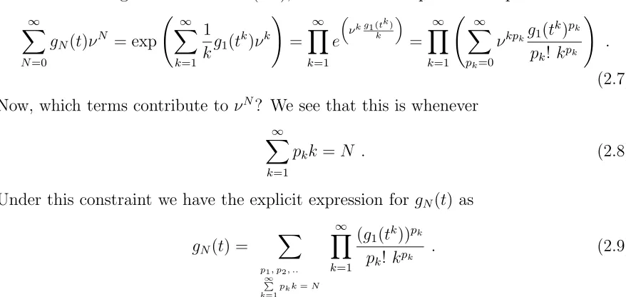
p=(0,1,0,1,0,2) N=18
[image:10.612.85.524.298.506.2]p=(1,2,0,1) N=9 p=(2,1,1,0,1) N=12
Figure 1: Examples of Young Tableaux with partitionp={p1, p2, p3, ..., pk, ...}and N. The
constraint is that N = P k=1
pkk.
2.2
Relation to Young Tableaux
One can proceed further with the above expansion for gN, and obtain interesting con-nections to Young tableaux. From (2.6), one can series-expand the exponential as:
∞ X
N=0
gN(t)νN = exp ∞ X
k=1
1 kg1(t
k)νk
!
= ∞ Y
k=1
e
„
νk g1(tk)
k «
= ∞ Y
k=1
∞ X
pk=0
νkpkg1(t
k)pk
pk! kpk
!
.
(2.7) Now, which terms contribute to νN? We see that this is whenever
∞ X
k=1
pkk =N . (2.8)
Under this constraint we have the explicit expression for gN(t) as
gN(t) =
X
p1, p2, ..
∞
P
k=1 pkk=N
∞ Y
k=1
(g1(tk))pk
pk! kpk . (2.9)
The relation (2.8) is a familiar combinatorial problem: the partition ofN into increasing components k = 1,2,3. . . of respective multiplicity pk. This is, of course, just the Young Tableau; to see it we just draw pk columns of length k from right to left with k increasing. For clarity, we have drawn a few illustrations in Fig. 1 with given p =
{p1, p2, p3, ..., pk, ...}. For example, for the first tableau, there is a total of 9 boxes. The
vector (1,2,0,1) means that p1 = 1, p2 = 2, p3 = 0 and p4 = 1. Now, p1 = 1 means that
there is 1 column with only one box; this is the first column from the right. Similarly, there are p2 = 2 columns with 2 boxes and p3 = 0 means there are no columns with 3
boxes. Finally, p4 = 1 means there is one column with 4 boxes, the one to the far left.
The reader is referred to the recent works of [11]. At a superficial level, we have related each term in the sum (2.9) to a given Young Tableau. In other words, given a Young Tableau we can count the number of columns with length k, say it is pk; then we can assign one factor (g1(tk))pk
pk!kpk . Multiplying all factors together we get contribution for the
particular Young Tableau. Finally we sum up all Young Tableaux with box number N, giving us the gN we need.
A Fermionic Version? As a brief digression, one notices that the expression for the plethstic exponential, in its product form, is a generating function for a bosonic oscillator. One might wonder what the fermionic counter-part signifies. In other words, we could define, for f(t) = P∞
n=0
antn,
g
P E[f(t)] := ∞ Y
k=1
(1 +tk)ak, P Eνg [f(t)] :=
∞ Y
k=0
(1 +νtk)ak .
It would be interesting to find what these may count in the D-brane gauge theory and what nice inverse functions they possess.
2.3
Generalising Meinardus
The asymptotic expressions for the generating functions are clearly of importance. In [4], we discussed at length the so-called Meinardus theorem [12] which generalises the Hardy-Ramanujan formula for the partition of integers and gives the asymptotics of the function g∞(t). Now, what about the aymptotic expressions of gN(t) where we have a finite number N of D3-branes? In other words, we wish to know, as n → ∞ in the expansion
gN(t) = ∞ X
n=0
gN(n)tn , (2.10)
the behaviour ofgN(n) for a given N.
THEOREM 2.1. For G(ν, t) = Q∞ r=1
(1−νtλr)−1 =
∞ P
n,N=0
gN(n)tnνN, define
Ψ(x) := logG(x) =−P∞
r=1
log(1−exλr),
K(x) := Q∞ r=1
1 + x λr
−1
ex/λr, F(y) := 1
2πi iR∞
−i∞
K(x)exydx,
ξ := a root of Ψ′(ξ) +n= 0 , N
0 :=
∞ P
r=1
(eξλr −1)−1,
then, the asymptotics (for n large and N fixed) are:
gN(n)∼ξF((N −N0)ξ) g(n), g(n)∼(2πΨ′′(ξ))−
1
2 eΨ(ξ)+nξ .
Of course, we need to recast our g(ν, t) in (2.4) into the form which the theorem addresses; this is a redefinition of theλr in terms of the am to eliminate repetitions:
λr=
1 r=a0, . . . , a1;
2 r=a1+ 1, . . . , a1+a2;
3 r=a1+a2+ 1, . . . , a1+a2+a3;
. . .
(2.11)
We see that the function G(x) = exp(Ψ(x)) is when the ν-insertion is absent (note that here counting does start from r = 1) and should capture the original Meinardus result for the plethystic exponential. Importantly, a key property of Ψ(x), in terms of the am coefficients (cf. [16]), is that its asymptotic behaviour is
G(x) =eΨ(x) = ∞ Y
r=1
(1−exr)−ar
∼expAΓ(α)ζ(α+ 1)x−α−D(0) logx+D′(0) ,
(2.12)
whereD(s) := P∞ m=1
am
ms is the Dirichlet series which has only 1 simple pole ats=α∈R+
with residue A.
Using (2.12) and its derivative, we see that the quantities ξand g(n) in Theorem 2.1 explicitly evaluate to, for large n,
ξ ∼ Root−AΓ(α+ 1)ζ(α+ 1)x−α−1−D(0)/x+n = 0 ∼
1
nAΓ(α+ 1)ζ(α+ 1)
1
α+1
g(n) ∼ C1nC2 exp
nαα+1(1 + 1
α) (AΓ(α+ 1)ζ(α+ 1))
1
α+1
C1 := eD
′(0) 1
p
2π(α+ 1)(AΓ(α+ 1)ζ(α+ 1))
1−2D(0) 2(α+1) , C
2 :=
D(0)−1− α
2
We see that g(n) above is exactly the Meinardus result [12, 16] for the asymptotics of the plethystic exponential withoutν-insertion (cf. also, Section 6 of [4]). In other words, the content of Theorem 2.1 is that the pre-factor
ξF((N−N0)ξ) (2.14)
encodes the effects of ν-insertion, i.e., the N-dependence, to the classical Meinardus asymptotic formula for g(n) in (2.13). For values of n < N the expression for gN(n) should coincide precisely with that of g∞(n) as the pre-factor tends to 1. On the other hand, forn > N there will be corrections and the gN(n) is expected to be smaller than g∞(n); this is because the counting should be less at finiteN since there are constraints which vanish at infinite N.
Example: C Let us first check a simple case. Let am = 1 for all m ∈ Z
≥0. This is
where the Hilbert series is equal tof∞(t) = (1−t)−1 and we recall [4] that the geometry
is just C. The conversion (2.11) makes λr = r, which is a specific example considered
on p238 of [13], giving us
K(x) = ∞ Y
r=1
1 + x r
−1
ex/r =eγxΓ(x+ 1), F(y) = exp −(γ+y)−e−(γ+y) ,
where γ := lim n→∞
n
P
j=1
j−1−log(n)
!
is the Euler constant1. The Dirichlet series is here
D(s) = P∞ m=1
m−s = ζ(s); whence α = A = 1 with D(0) = −1
2 and D′(0) = − 1
2log(2π).
Therefore, (2.12) dictates that
Ψ(x)∼ π
2
6x + 1
2logx− 1
2log 2π⇒Ψ
′(x)∼ − π2 6x2 +
1 2x, Ψ
′′(x)∼ π2 3x3 −
1 2x2 .
By (2.13) we thus have
ξ ∼ −3 +
√
24nπ2+ 9
12n ∼
π
√
6n , g(n)∼(2πΨ
′′(ξ))−1
2 eΨ(ξ)+nξ ∼ 1
4√3ne
π√2n/3 .
(2.15) Indeed, g(n) is exactly the famous Hardy-Ramanujan asymptotic behaviour for the η-function. The effect of the ν-insertion is then apparent in the pre-factor governed by
1 Indeed, we can see this sinceF(y) = P
n=−1,−2,−3,...
Res
z→nΓ(z+ 1)e
γz+zy = P∞ n=0
(−1)n
n! e−(n−1)(γ+y)=
the function F. Now, we see that, for small x,
N0(x) =
∞ X
r=1
(exp(rx)−1)−1 ∼
1/x X r=1 1 rx+ ∞ X
r=1/x
exp(−rx) =−H(1/x)
x +
ex−1
ex−1 ∼ − logx
x , (2.16) where we have series-expanded for the first part of the sum (H(x) is the Harmonic number) and neglected the small contribution of the −1 in the denominator for the second sum. Therefore, since n is large, we can apply (2.16) to give us
N0 =N0(ξ)∼
√ 6n π log √ 6n π .
Thus, we can write the pre-factor in (2.14) (n is large and N is fixed) as
ξF ((N −N0)ξ) ∼ √π6nexp
−(γ+ (N −N0)√π6n)−e−(γ+(N−N0)
π √
6n)
∼ √π
6nexp
log√π6n − √N π
6n−e
log√6n
π −
N π √
6n
∼exp(−√N π
6n − √
6n π e
−√N π
6n) .
In summary, we have the asymptotic expansion ofgN(n) as
gN(n;C)∼ 1
4√3nexp π
r 2n 3 ! exp " −√Nπ
6n −
√
6n π e
−√N π
6n
#
. (2.17)
We have actually reproduced a classical result of [17], which is also studied recently in Bose-Einstein condensates in [18]. Specifically, the above result agrees completely with Eq.(13) of [18], wherein they have simplified the expression to g√(n)
n exp(−
2
c exp(xN(n))− xN(n)) with c=q23π, g(n) given in (2.15) andxN(n) := 2cN√
n−log(
√
n).
2.4
A Large Class of Examples
Thus emboldened, we may proceed to more examples. Since the plethystic exponential has a singularity att= 1 at ν = 1, it is expedient to study contributions of the form
f(t) =f∞(t;M) =g1(t;M) =
V3
(1−t)3 +
V2
(1−t)2 +
V1
1−t +V0+O(1−t) ; (2.18) we go up to poles of order 3 becauseMis at most 3-dimensional in the cases of concern. Physically, V3 can be thought of as the volume of the dual AdS horizon, i.e., the
It turns out, for what we shall shortly describe in the next section, that we do not need as refined an attack as Haselgrove-Temperley, but, rather, a leading order analysis. Indeed, the results of [13] for d > 1 require a regularisation into whose subtleties we presently do not wish to venture. We shall, instead, follow the saddle-point method in the physics literature, such as [19]. Indeed we are essentially studying a contour integral
gN(n) = 1 (2πi)2
I
Γν=0
dν
I
Γt=0
dt g(ν, t) νN+1tn+1 ,
which picks up the residues at the poles and the form in (2.18) will be dominant. The statement, with the same notations as above, is as follows. For both N and n large (note that Haselgrove-Temperley only requires thatn be large),
gN(n)∼g(ν0, t0)ν0−N−1t−0n−1, where
N + 1 =ν ∂
∂ν logg(ν, t)
ν0,t0
,
n+ 1 =t ∂
∂t logg(ν, t)
ν0,t0
. (2.19)
We can first directly evaluate logg(ν, t). From (2.18), we have that
an = V3
(n+ 1)(n+ 2)
2 +V2(n+ 1) +V1+V0δn,0 ⇒ logg(ν, t) = −
∞ X
n=0
anlog(1−νtn)
= −V0log(1−ν) +
∞ X k=1 νk k 1
2V3Li−2(t
k) + (V
2+
3
2V3)Li−1(t
k) + (V
1+V2+V3)(1 +Li0(tk))
,
where we have used the definition of the Polylogarithmic function Lid(x) = ∞ P
n=1
xn
nd. In
fact, for d∈Z
≤0, these are simply rational functions.
Recall now that we wish to study the behaviour of g(ν, t) near t = 1 and ν = 1. Hence, we can define t:=e−q and ν =e−w and will study the behaviour near q, w→0. Series expanding logg(ν, t) and keeping dominant contributions in the inverses of qand w, we find that
logg(w, q) ∼ ∞ X k=1 νk k
V0+
V1
2 + 5V2
12 + 3V3
8 +
V1+V2+V3
k q +
2V2+ 3V3
2k2q2 +
V3
k3q3
∼ V3
q3(ζ(4)−ζ(3)w)−(V0+
V1
2 + 5V2
12 + 3V3
8 ) log(w) . (2.20)
e−w, we have t∂ ∂t =−
∂
∂q and ν ∂ ∂ν =−
∂
∂w and the saddle equations read:
n+ 1 = −∂logg(w, q)
∂q ∼3ζ(4)V3q −4 ,
N + 1 = −∂logg(w, q)
∂w ∼ζ(3)V3q
−3+ (V 0+
V1
2 + 5V2
12 + 3V3
8 )w −1 .
Therefore, the saddle points are
q0 ∼
3V3ζ(4)
n
1 4
, w0 ∼(V0+
V1
2 + 5V2
12 + 3V3
8 ) N −ζ(3)V3q −3 0
−1
(2.21)
These results are encouraging. For V0,1,2 = 0 and V3 = 1, the case was studied in nice
detail in [19]. The expressions in (2.21), to leading order, agree exactly with their Eq. (17-19), in cit. ibid. Substituting back into (2.19), we conclude that, to leading order,
loggN(n) ∼ logg(ν0, t0) +Nw+nq
∼ C0n
3 4 +C
1
N N −C2n
3 4
+ logN−C2n
3 4
; (2.22)
C0 := 3−
3
44(V3ζ(4)) 1
4, C1 :=V0+V1
2 + 5V2
12 + 3V3
8 , C2 :=ζ(3)V
1 4
3 (3ζ(4))−
3 4 .
Once more, we are re-assured. The first term, which only depends on n, should be the classical Meinardus result while the second is the pre-factor (2.14) discussed above. We have done the Meinardus analysis for C3 in [4]; substituting ζ(4) = π4
90 gives us the first
term as 2·2
3 4π
3·1514 n 3
4, precisely the exponent of p1 in Eq (6.7) of [4].
Another interesting limit to consider is t ∼ 1 and ν ∼ 0. Here, we expand about q=−logt and ν directly and (2.20) becomes
logg(ν, t)∼νV3q−3 , (2.23)
giving us the saddle points q0 ∼3N/nand ν0 ∼(3N/n)3N/V3. Thus,
loggN(n)∼4N
log(N−1n34) + 1− 1
4log 27 V3
. (2.24)
Note that in order forν ∼0, we need N ≪n34.
2.5
The Entropy of Quiver Theories
Meinardus, let us now address a problem of great physical interest. A chief motivation for finding explicit expressions, in paricular the asymptotic behaviour, of our generating functions is to determine the number of degrees of freedom, i.e., the entropy of the gauge theory. Indeed, as the Hardy-Ramanujan formula is central to the determining the entropy of the bosonic critical string, the results presented in the previous section will be essential to that of D-brane probe theories.
The growth of the number of our mesonic BPS operators in the gauge theory can be a good estimate for the entropy of the system. More generally, it serves as a lower bound for the total number of operators in the gauge theory, regardless of whether they are BPS or not. Thus if we are looking for an underlying black hole entropy, the discussions above will be greatly pertinent. Specifically, in our context of the gauge theory of N D-branes probing a geometryM, we can define the entropy SN(n) as
SN(n) = loggN(n) where g(ν, t;M) := ∞ X
N,n=0
gN(n)tnνN , (2.25)
and we recall thatg(ν, t;M) is theν-inserted plethystic exponential of the Hilbert series (the fundamental generating function f) of the geometry of M.
Now, we would like to compute critical exponents depending on dimensionality. Therefore, we need to consider the generalisation of (2.18) to
f(t) = Vd
(1−t)d +. . .+ V2
(1−t)2 +
V1
1−t +V0+O(1−t) . (2.26) Following the computation performed above, we easily see that the saddle points are (in the t, ν ∼1 limit) now
q0 ∼
dVdζ(d+ 1) n
1
d+1
, w0 ∼
"
V0+
d
X
j=1
Vj(1 + j−1
X
i=0
βiζ(−i))
#
N −ζ(d)Vdq0−d−1 , (2.27) whereβi are coefficients such that
n+d−1 d−1
:= d−1
X
i=0
βini . (2.28)
Substituting into the saddle point equation, we find the entropy to be
SN(n)∼C0nα+C1
N N−C2nα
+ log (N −C2nα)
where the critical exponent is α= d
d+1 and the constants are
C0 = d−
d
d+1(d+ 1)(Vdζ(d+ 1)) 1
d+1 ,
C1 = V0+
d
X
j=1
Vj(1 + j−1
X
i=0
βiζ(−i)) ,
C2 = ζ(d)V
1
d+1
d (dζ(d+ 1))−
d d+1 .
We remark, upon obtaining a similar expression as (2.24) forν ∼0, that our treatment gives rise to a critical regime in which there is a cross over betweenν∼0 andν∼1. This critical regime is given by the order parameterN ∼nd/d+1 or, alternatively,n ∼N1+1/d. When the two sides are of the same order we are in theν ∼1 regime and the number of operators is controlled byn essentially. When the order parameter is small the number of operators depends on N.
3
SU
(2)
Subgroups: ADE Revisited
We have, in the above, discussed extensively the various general properties of the gener-ating functions, the recursions, relations to Young tableaux, and especially the asymp-totics. Now, let us move on to some specific examples. An extensively studied class of CY singularities are orbifold theories. Of particular mathematical interest has been the local-K3 singularities, viz.,C2/Gwhere Gis a discrete, finite subgroup ofSU(2). Such
groups fall under an ADE-pattern and the quivers are central to the McKay Correspon-dence.
In [4], we computed the fundamental generating functions, i.e., the Hilbert series g1 = f∞. We recall that for orbifolds of finite group G, the Hilbert series is computed by the so-called Molien series
f∞(t;G) =M(t;G) = 1
|G|
X
g∈G
1
det(I−tg) . (3.1)
A natural question to ask is what explicit expressions can be derived for gN at finite N. Using the prescription in the previous section, we can readily expand a few terms of (2.7) to see what we obtain. Take the example of G= ˆD4, the binary dihedral group of
order 8, which was investigated in detail in [4], the Hilbert series is the Molien series
g1(t) =M(t; ˆD4) =
1 +t6
Substituting (3.2) into (2.7), we obtain (g0(t) = 1 automatically):
g2(t) =
1−t2+t6+t8−t12+t14
(1−t2) (1−t4)2 (1−t8) , g3(t) =
1−t2+ 2t8+t12+t18+ 2t22−t28+t30
(1−t2) (1−t4)2 (1−t6) (1−t8) (1−t12) , . . .
We see that these coefficients quickly become complicated. Nevertheless, the algorithm is clear and one may extract gN ad libertum.
3.1
Recursion Relations and Difference Equations
Let us entice the reader with some immediately noticeable curiosities for the series-coefficients for the Hilbert (Molien) series for the ADE orbifolds. Take the A-family (where ˆAn−1 :=Zn). We recall from [4] that
f∞(t; ˆAn−1) =
(1 +tn) (1−t2)(1−tn) . We see that
f∞(t; ˆA1) = 1 + 3t2+ 5t4+ 7t6+ 9t8+ 11t10+ 13t12+ 15t14+ 17t16+ 19t18+ 21t20+O(t21)
f∞(t; ˆA3) = 1 +t2+ 3t4 + 3t6+ 5t8+ 5t10+ 7t12+ 7t14+ 9t16+ 9t18+ 11t20+O(t21)
f∞(t; ˆA5) = 1 +t2+t4+ 3t6+ 3t8+ 3t10+ 5t12+ 5t14+ 5t16+ 7t18+ 7t20+O(t21)
(3.3) Thus, forn = 2k even, the pattern of the coefficients is{1, . . . ,1; 3, . . . ,3; 5, . . . ,5;. . .}. In fact, we will now proceed to find analytic expressions for the series-coefficients, i.e., the number of single-trace GIO’s, of f∞ for all the discrete, finite subgroups of SU(2). This indeed places our generating function in full power and provide us with invariants of arbitrary degree immediately. The reason we can do so is because the Molien series is a rational function int and indeed, for any rational function, one could systematically obtain recursion relations, which can then be solved. It is easiest to start with the exceptionals, i.e., the E-family, with which we shall commence our illustration.
The Eˆ6 Singularity: For ˆE6, we recall from [4] that
f = 1−t
4+t8
1−t4−t6+t10 = 1 +t
6+t8+ 2t12+t14+O(t16) :=
∞ X
k=0
Multiplying through by the denominator gives us
1−t4+t8 = ∞ X
k=0
aktk− ∞ X
k=4
ak−4tk−
∞ X
k=6
ak−6tk+
∞ X
k=10
ak−10tk (3.5)
=
9
X
k=0
aktk−
9
X
k=4
ak−4tk− 9
X
k=6
ak−6tk+
∞ X
k=10
(ak−ak−4−ak−6+ak−10) .
Identifying the coefficients of powers of t, this readily gives us the recursion relation:
ak =ak−4+ak−6−ak−10, k ≥10. (3.6)
There should be 10 initial conditions for ak, which could be obtained by matching the 1 as well as the −t4 and t8 terms in the LHS with the various finite sum pieces in the
RHS of (3.5). Alternatively, it is easier to simply read off the first 10 values ofak in the series expansion in (3.4), giving us
a0,6,8 = 1, else, ak<10= 0 .
Of course, all linear homogeneous difference equations of this kind can be solved. Upon substitution of the ansatz ak =tk for some t∈C, one obtains the eigen-equation for t which is simply the denominator 1− t4 − t6 +t10 in (3.4). This has 10 roots:
{ω6i=0,...,5,±i}with double roots at 1 and−1. Using the usual trick that for each multiple rootλ of order m, there are extra roots kj=1,...,m−1λk, the solution is reaily found to be ak = (−1)k (c(1) +k c(2)) +c(3) +k c(4) +c(5) cos(k π
3 ) +
c(6) cos(k π
2 ) +c(7) cos( 2k π
3 ) +c(8) sin( k π
3 ) +c(9) sin( k π
2 ) +c(10) sin( 2k π
3 ) ,
with initial constants c(i), i = 1, . . . ,10. Matching these with the 10 initial conditions in (3.6) gives us the final solution
ak = 1 72
31 + (−1)k (1 +k) + 18 cos(k π 2 ) + 24
cos(k π
3 ) + cos( 2k π
3 )
+
+8√3
sin(k π
3 )−sin( 2k π
3 )
, k = 0,1, . . .
There is an obvious cyclicity of 12 and a12m = 1 +m for m∈ Z≥0. We will shortly see
The Eˆ7 Singularity: For ˆE7, we have [4] that
f = 1−t
6 +t12
1−t6−t8+t14 = 1 +t
8+t12+t16+t18+t20+ 2t24+t26+t28+t30+ 2t32+
O(t34), giving us the recursion relations
ak=ak−6+ak−8−ak−14, k≥14, a0,8,12= 1, else, ak<14= 0 . (3.7)
This can be readily solved using the above methods to be, for k= 0,1, . . .,
ak = 1 144
31 + (−1)k (1 +k) + 2 cos(k π 2 )
27 + 24 cos(k π 6 )+
18
cos(k π
4 )−sin( k π
4 )
−8√3 sin(k π 6 )
.
Again, there is an obvious cyclicity of 24 and a24m = 1 +m for m∈Z≥0.
The Eˆ8 Singularity: For ˆE8, we have that [4]
f = 1 +t
2−t6−t8−t10+t14+t16
1 +t2 −t6−t8−t10−t12+t16+t18 = 1 +t
12+t20+t24+t30+t32+t36+t40+t42+
t44+t48+t50+t52+t54+t56+ 2t60+t62+O(t64) , giving us the recursion relations
ak =−ak−2+ak−6+ak−8+ak−10+ak−12−ak−16−ak−18 k≥18, a0,12= 1, else, ak<18= 0.
Again, this can be solved exactly, giving us, fork = 0,1, . . .,
ak = 1 1800
"
15 1 + (−1)k (1 +k) + 36
r
55−2√5 sin(2k π
5 )−sin( 3k π
5 )
+
+36
r
5 5 + 2√5 sin(k π
5 )−sin( 4k π
5 )
+
+10 cos(k π 2 )
45 + 36
cos(k π
10) + cos( 3k π
10 )
+ 60 cos(k π 6 )−20
√
3 sin(k π 6 )
.
Once more, there is an obvious cyclicity of 60 anda60m = 1 +m for m ∈Z≥0.
The Aˆn Family: Now, let us move on to the infinite families. For, ˆAn−1, we have
that, lettingf∞(t; ˆAn) = (1−(1+t2)(1tn−)tn) :=
∞ P
k=0
aktk,
1 +tn = P∞ k=0
aktk− P∞ k=2
ak−2tk−
∞ P
k=n
ak−ntk+ P∞ k=n+2
ak−n−2tk
= (a0+a1t+. . .+an+1tn+1)−(a0t2+a1t3+. . .+an−1tn+1)−
−(a0tn+a1tn+1) +
∞ P
k=n+2
(ak−ak−2−ak−n+ak−n−2)tk .
Identifying coefficients oft, we have that
ak =ak−2+ak−n−ak−n−2, k ≥n+ 2 ; (3.9)
we still need n+ 2 initial conditions. One is obvious, a0 = 1, the remaining can be
obtained by solving for the system of associated equations above for a1, . . . , an+1.
Now, we could solve this recursion equation, which is rather difficult because of the determination of these initial conditions. However, in this case, it is far easier to simply observe the pattern and conclude that
n = odd ak = floor(nk) + 12 1 + (−1)mod (k,n)
n = even ak= floor(nk+ 21) 1 + (−1)mod (k,n) (3.10)
Again, the cyclicities are apparent: for odd n, ak=2βn = 2β and for even n, ak=2βn = 4β+ 1 forβ ∈Z≥0. We will write these coefficients explicitly later using the MacMahon
and Dedekind functions in§3.2.
The Dnˆ Family: For the ˆDn+2 groups, the recursion relation reads
f∞(t; ˆDn+2) =
(1 +t2n+2)
(1−t4)(1−t2n) := ∞ X
k=0
aktk, ak =ak−4+ak−2n−ak−2n−4; k ≥2n+4,
(3.11) together with 2n+ 4 initial conditions.
Once again, it is easier to directly observe the pattern here. First, we notice that, upon making the substitution t2 →t, the Hilbert series becomes quite analogous to the
A-series. Indeed, in analogy to (3.3), we find that the coefficients for even n come in periodicity of order n and that for the k-th period the even coefficients are 2k+ 1 and the odd coefficients are 0. We will use this in writing expressions for the generating function in §3.2.
In summary, we may observe the pattern of the expansion coefficients as:
(1 +tn+1)
(1−t2)(1−tn) := ∞ X
k=0
bktk ⇒ bk = 1
2 1 + (−1)
k+floor
1
n mod (k,2n)
+2 floor
k 2n
.
(3.12) Therefore, upon restoringt →t2, we only have even powers; whence, for allk = 0,1, . . .,
ak =
(
0, k odd;
1
2 1 + (−1)
k/2+ floor 1
n mod (k,4n)
+ 2 floor k
4n
3.2
Full Generating Functions: MacMahon and Euler
Having obtained analytic expressions for the counting of single-trace GIO’s, i.e., the coefficient of the fundamental generating function f∞, the Hilbert series, we can say something further about the plethystic exponentials. The expressions for the ADE orbifolds can be represented as infinite sums. Such sums appear in different counting formulae for integer partitions under special restrictions. For example, it is not surprising to find that the multi-trace generating function forC2,
g∞(t;C2) = exp
X∞
n=1
1
n (1−t n)−2
−1
= 1+2t2+6t3+14t4+33t5+70t6+. . . (3.14) generates the sequence of the number of partitions of n objects with 2 colors [24]. It would be interesting to find similar results for the ADE series.
Now, we can use an alternative representation for the generating functions such as (2.4). For the exmaple of C2, we recall that
g(ν;t;C2) =
∞ Y
n=0
(1−νtn)−(n+1).
We note that the coefficients an have a linear piece and a constant piece. This property turns out to be generic for all 2 dimensional singular manifolds. We will therefore define two basic functions. First, let the generalized MacMahon function be:
M(ν;t) := ∞ Y
n=1
(1−νtn)−n ; (3.15)
next, let the generalized Dedekind Eta function (in this form it is actually the generalised Euler function, which differs from the Eta function by the famous factor of t−1/24) be
defined as:
η(ν;t) := ∞ Y
n=0
(1−νtn)−1 . (3.16)
In terms of these functions we can now rewrite
g(ν;t; C2) =M(ν; t)η(ν; t) .
Let us look, for example, at the generating function for C2/Z2. We find that
g(ν;t; C2/Z2) =
∞ Y
n=0
(1−νt2n)−(2n+1) , which can be easily rewritten as
g(ν;t; C2/Z2) =M(ν;t2)2η(ν;t2) .
To proceed with the full A-family, we now use the periodic pattern for the coefficientan which was obtained above in (3.10), and obtain the following succint expression for the generating functiong(ν, t):
g(ν;t;C2/Z2k) =
k−1
Y
j=0
M(νt2j;t2k)2 η(νt2j;t2k)
g(ν;t;C2/Z2k+1) = 2k
Y
j=0
M(νtj;t2k+1) k
Y
j=0
η(νt2j;t2k+1)
Similarly, we can obtain the full-generating function for the D-family:
g(ν, t;C2/Dˆ2k) = 2Yk−3
j=0
M(νt2j;t4k−4) k−2
Y
j=0
η(νt4j;t4k−4)
g(ν, t;C2/Dˆ2k+1) = 4Yk−3
j=0
M(νt2j;t8k−4)2
2Yk−2
j=0
η(νt4j;t8k−4)
2Yk−2
j=0
η(νt2j+4k−2;t8k−4) .
Finally, for the E-family, as mentioned above we find that each of the Hilbert series come with a quasi-periodicity of 12, 24, and 60 for ˆE6,7,8, respectively, which can be seen
from the explicit expressions for the coefficients in the various equations for ak given in the previous subsection. The growth of the coefficients is always linear in these periods. Furthermore, odd powers never appear. Therefore, one can write vectors of length 6, 12, and 30, which will denote the starting powers of the coefficients. Explicitly, we have:
vE6 = {1,0,0,1,1,0}
vE7 = {1,0,0,0,1,0,1,0,1,1,1,0}
The generating functions then take the form
g(ν, t;C2/Eˆ6) = 5
Y
j=0
M(νt2j;t12)η(νt2j;t12)vjE6
g(ν, t;C2/Eˆ7) = 11
Y
j=0
M(νt2j;t24)η(νt2j;t24)vjE7
g(ν, t;C2/Eˆ8) = 29
Y
j=0
M(νt2j;t60)η(νt2j;t60)vjE8 .
Two curiosities are perhaps worthy of note. First, the periodicities of the coefficients in the Hilbert series are, respectively, one half the order of the finite groups themselves. Second, for each of the vectorsvE6,E7,E8 above, one can draw a line at the middle, then
upon mirror reflection about this line, a zero is mapped to a one, and vice versa.
3.3
Asymptotic Expansions for
g
∞As was emphasised in [4] as well as the proceeding discussions, the asymptotic behaviour ofg∞is of great interest. Using the Meinardus Theorem, we can estimate the asymptotic behaviour for g∞ for the ADE-singularities. Though the expressions for the ak are, evidently, quite involved, the large k behaviour is dominated by the term proportional tok, which can be directly observed; other eigenvalues have less than unit modulus and decay ad nullam. We wish to find dm in
∞ Y
k=1
1
(1− tk)ak :=
∞ X
m=0
dmtm
for large m.
It suffices to see the largek behaviour ofak for the ADE-orbifolds. We see, from the expressions above, that allakare essentially linear in k. For ˆAn−1,nodd, the coefficient
of the linearity is simply 1/n. For all other cases, the coefficient is the reciprocal of 1/2 the order of the group. However, for all these cases, exactly 1/2 of the terms are zero and contribute 1 to the product. Therefore, overall, the effective large k-behaviour is still simply the reciprocal of the order of the group. Hence, we conclude that
For G=ADE, ak∼ k
Now, we are at liberty to use the Meinardus analysis. For ak∼k, we recall from [4] that this is the case of the MacMahon function, whose behaviour goes as
∞ Y
k=1
1
(1− tk)k := ∞ X
m=0
ϕ(m)tm, ⇒ ϕ(m)∼ 2−
11 36ζ(3)
7 36e121
Gl√3π m
−2536 exp
3
2(2ζ(3))
1 3m23
,
(3.18) with Gl := 121 −ζ′(−1) being the Glaisha constant. Thus, we see that for G being an ADE-group,
dm ∼ϕ(m)|G1| . (3.19)
In fact, taking the logarithm of this expression will give us the entropy of the quiver gauge theory as discussed in§2.5. We conclude that the entropy is reduced by a factor of |G|and this is the natural expectation from an extensive parameter like the entropy since, by the orbifold action, we are losing |G| of the degrees of freedom.
Incidentally, the MacMahon function is the generating function for the plane-partition problem which is a generalisation of the Young Tableaux to 2-dimensions. That is, con-sider an integer m, how many ways are there to write
m =X i,j
ni,j such that ni+1,j ≥ni,j, ni,j+1 ≥ni,j; ni,j ∈Z+ .
The answer was shown in [25] to be precisely ϕ(m). The 1-dimensional partition prob-lem, i.e., how many Young Tableaux (also called Ferrers Diagram) are there of a given total number of squares, is simply the standard partitioning problem. By this we mean how many ways, irrespectively ordering, are there to write a given integer m as sums of integers. This is because we could always order the parts in decreasing fashion and arrive at a Young Tableau. The generating function here is simply the famous Euler function Q∞
k=1 1
(1−tk). It is a curious fact that 3 and higher dimensional analogues of the
problem remain unsolved. A conjecture was made in [25] which was later shown to be incorrect.
3.4
The MacMahon Conjecture
One could imagine what the result for solid-partitions, which, as mentioned above, is unknown, might actually be. Let us tabulate the result for the gauge theories forCand C2. We recall from [4] that
f∞(t; C) = 1
1−t = ∞ X
k=0
tk, ⇒ g∞(t; C) =
∞ Y
k=1
1 (1− tk);
f∞(t; C2) = 1
(1−t)2 =
∞ X
k=0
(k+ 1)tk, ⇒ g∞(t; C2) =
∞ Y
k=1
1 (1− tk)k+1 .
Thus we see that the multi-trace problem forCcounts the 1-dimensional partition; that
for C2, when shifted by 1, counts the 2-dimensional problem. It is perhaps natural to
guess that the one for C3, when shifted by one, would give the generating function for
the 3-dimensional partition problem, i.e.,
f∞(t; C3) = 1
(1−t)3 =
∞ X
k=0
(k+ 1)(k+ 2)
2 t
k, shift⇒a k =
k(k+ 1)
2 ⇒ (3.20)
g∞ = ∞ Y
k=1
1
(1− tk)k(k2+1) = 1 +t+ 4t
2+ 10t3+ 26t4+ 59t5+ 141t6+ 310t7+ 692t8+O(t9) .
Unfortunately, this leads us back to MacMahon’s erroneous guess [25]. The correct numbers, as generated by exhaustive computer simulation of the explicit partitions, should be (cf. e.g. [26]):
1,1,4,10,26,59,140,307,684,1464,3122,6500,13426,27248,54804,108802, . . . (3.21)
One sees that starting from the term 141, the generating function g∞ in (3.20) over-counts. The actual series ak which does generate the correct numbers can be easily found, by taking the plethystic logarithm, to be (cf. also [26])
ak=1,2,... = {1,3,6,10,15,20,26,34,46,68,97,120,112,23,−186,−496,
4
All
SU
(3)
Subgroups
We have discussed the ADE-groups above in some detail; of perhaps more physical interest are the orbifolds of C3. These are local Calabi-Yau threefolds that give rise to
N = 1 4-dimensional chiral gauge theories on the D3-brane world-volume. The quiver theories were studied in [23] and using the notation therein, the discrete finite subgroups of SU(3) are:
(I) The infinite family Zm×Zn;
(II) The infinite families ∆(3n2) and ∆(6n2);
(III) The exceptionals Σ60, Σ108, Σ168, Σ216, Σ648, and Σ1080.
The theory of Molien series and algebraic invariants is nicely exposed in [6], wherein some explicit Molien series are also computed for the discrete subgroups of SL(3;C).
In order to explicitly write the generators of the groups, first, define
ωn:= exp( 2πi
n ),
and the matrices
S :=
1 0 0
0 ω3 0
0 0 ω3 2
, S1 :=
1 0 0
0 ω54 0
0 0 ω5
, S2 :=
ω
7 0 0
0 ω72 0
0 0 ω7 4
;
T :=
0 1 0
0 0 1 1 0 0
, T1 := √15
1 1 1
2 1 2(−1−
√
5) 1 2(−1 +
√
5) 2 1
2(−1 + √
5) 1 2(−1−
√
5)
, T2 :=
1 0 0 0 0 1 0 −1 0
!
;
R :=−√1
−7
−ω73+ω74 ω72−ω75 ω7−ω76 ω7
2 −ω7
5
ω7−ω7 6
−ω7 3
+ω7 4
ω7−ω7 6
−ω7 3
+ω7 4
ω7 2
−ω7 5 ; U := ω9 4 0 0 0 ω94 0
0 0 ω3ω9 4
, U1 :=
−1 0 0 0 0 −1 0 −1 0
;
V := √1 −3
1 1 1
1 ω3 ω32
1 ω3 2
ω3
, V1 := √15
1 1
4(−1 + √
−15) 1 4(−1 +
√ −15)
1 2(−1−
√
−15) 1 2(−1−
√
5) 1 2(−1 +
√
5)
1 2(−1−
√
−15) 1 2(−1 +
√
5) 1 2(−1−
√ 5) ; A(m) := ω
m 0 0
0 1 0 0 0 ω−1
m
, B(n) :=
1 0 0
0 ωn 0
0 0 ω−1
n
.
Finally, we adhere to the usual notation that
G=hg1, . . . , gki is the finite groupG generated by matrices g1, . . . gk.
4.1
The Abelian Series:
Z
m×
Z
nThe first of our series is simplyZm×Zn =hA(m), B(n)i. The Molien series is given by
f(t; Zm×Zn) = 1
mn mX−1
i=0
n−1
X
j=0
det
I3×3−t
ωi
m 0 0
0 ωj
n 0
0 0 ω−i mω −j n −1 (4.2) = 1 mn mX−1
i=0
n−1
X
j=0
1 (1−tωi
m)(1−tω j
n)(1−tω−i mω−
j n )
= 1
mn m−1
X
i=0
n−1
X
j=0
∞ X
p,q,r=0
tpωmiptqωjqntrωm−irω−njr .
Using the identity
mX−1
i=0
ωmix =mδx,mZ ,
where the Kronecker-Delta is 1 whenever xis a multiple of n, we can see that non-zero contributions come from
p=r+p me forpe=−[r m],−[
r
m] + 1, . . .; q=r+q ne for eq=−[ r n],−[
r
n] + 1, . . . . Here, [r
m] means to take the integer part (i.e., floor(r/m)). Whence,
f(t; Zm×Zn) =
∞ X r=0 ∞ X e
p=−[mr]
∞ X
e
q=−[rn]
t3r+p me +eq n= ∞ X
r=0
t3r−[r m]m−[
r n]n
(1−tm)(1−tn) .
To go further, we can writer=er+LCM(m, n)zforz = 0,1, ...,∞ander= 0,1, ..., LCM(m, n)− 1, where LCM is the lowest common multiple. Using this parametrization, the sum
re-duces to
f(t; Zm×Zn) = 1
(1−tm)(1−tn)
LCM(m,n)−1
X e r=0 ∞ X z=0
t3er−[mre]m−[e r
n]ntLCM(m,n)z (4.3)
= 1
(1−tm)(1−tn)(1−tLCM(m,n))
LCMX(m,n)−1
e
r=0
t3er−[re m]m−[e
r n]n .
The above expression becomes particularly simple in the case of perhaps greatest inter-est, viz, when m =n; here LCM(m, n) =m and within the range of summation of r,e [er
m] is zero, hence
f(t; Zm×Zm) = 1−t 3m
Taking the plethystic logarithm of (4.4) gives polynomials, suggesting thatC3/(Zm×Zm)
are all complete intersections! Explicitly, we have that
f1(t; Zm×Zm) =P E−1[f(t; Zm×Zm)] =
3t m = 1,
3t2+t3−t6 m = 2,
4t3−t9 m = 3,
t3+ 3tm−t3m m ≥4.
(4.5)
The m= 1 case is a good check; this is simply the result for the parent C3 theory.
Refinement: As was pointed out in [4], where there are enough isometries, as cer-tainly is the case with toric varieties, refinements can be made to the Molien series. The above Abelian series are indeed toric, hence one could write the refined Molien (Hilbert) series as
f(t1, t2, t3; Zm×Zn) = 1 mn
mX−1
i=0
n−1
X
j=0
det
I3×3−
t
1 0 0
0 t2 0
0 0 t3
ωi
m 0 0
0 ωj
n 0
0 0 ω−i mω
−j n
−1
.
This can, using the above reparametrisation of the summation variables, be re-written as
f(t1, t2, t3; Zm×Zn) =
1 (1−tm
1 )(1−tn2)(1−t
LCM(m,n)
3 )
LCM(m,n)−1
X
e
r=0
(t1t2t3)ert− [re
m]m
1 t
−[re n]n
2 .
Once again, for the case of m=n, the expression simplifies considerably:
f(t1, t2, t3; Zm ×Zm) =
1−(t1t2t3)m
(1−t1t2t3)(1−t1m)(1−tm2 )(1−tm3 )
. (4.6)
The plethystic logarithm of this expression becomes particularly simple:
f1(t1, t2, t3; Zm×Zm) =tm1 +tm2 +tm3 +t1t2t3−(t1t2t3)m , m= 1,2,3, . . . (4.7)
4.2
Non-Abelian Subgroups
Having expounded upon theZm×Znseries in detail, we can proceed to the non-Abelian
The elements of ∆(3n2) := hA(n), B(n), Ti fall into three classes, viz, the orbits of Z2
n≃ hA(n), B(n)iunder{I, T, T2}since the matrixT, which we recall from (4.1), is of order 3. Therefore,
f(t; ∆(3n2)) = 1 3n2[
n−1
X
i,j=0
det
I3×3−t
ωi
n 0 0
0 ωjn 0 0 0 ω−i−j
n
−1
+ det
I3×3−t
0 ωj
n 0
0 0 ω−i−j n
ωi
n 0 0
−1
+ det
I3×3−t
0 0 ω−i−j n
ωi
n 0 0
0 ωnj 0
−1
]
= 1
3n2
n2 1−t
3n
(1−t3)(1−tn)3 +n 2 1
1−t3 +n 2 1
1−t3
= 1−t
n+t2n
(1−t3)(1−tn)2 . (4.8)
One could in fact take the plethystic logarithm and see that these are complete inter-sections:
f1(t; ∆(3n2)) =P E−1[f(t; ∆(3n2))] =
t+t2+ 2t3−t6 n = 1,
t2+t3+t4 +t6 −t12 n= 2,
2t3+t6+t9−t18 n= 3,
t3+tn+t2n+t3n−t6n n ≥4.
(4.9)
In complete analogy, ∆(6n2) := hA(n), B(n), T, T
2i. In fact ∆(6n2) ≃ ∆(6(2n)2),
thus it suffices to consider only odd n, and we have that
f(t; ∆(6n2)) = 1 +t
6n+3
(1−t6)(1−t2n)(1−t4n), n = 1,3,5, . . . . Again, taking the plethystic logarithm shows these to be complete intersections
f1(t; ∆(6n2)) =P E−1[f(t; ∆(6n2))] =
t2 +t4+t6 +t9 −t18 n= 1,
2t6+t12+t21−t42 n= 3,
t6+t2n+t4n+t6n+3−t12n+6 n≥5.
(4.10)
4.3
Summary of
SU
(3)
Subgroups
fact is that all of them (except Zm×Zn for m 6= n, whose Molien series we have not
been able to simplify further) are complete intersections. We use the notation (cf. [35] for gauge theory moduli spaces of this type)
(p,(d1, . . . , dk); (ℓa11, . . . , ℓaqq))
to denote the intersection of k equations, of degrees d1, . . . , dk in Cp, composed of a1
invariants of degree ℓ1, a2 invariants of degree ℓ2, etc.
The generating functions (Molien series) f = f∞(t) and the associated f1 which
encode the syzygies (defining equations) for the discrete, finite subgroups of SU(3) are:
G⊂SU(3) Generators Molien f(t;G) f1 =P E−1(f) Defining Equation
Zm×Zn hA(m), B(n)i q.v. (4.3) q.v. (4.5) −
∆(3n2) hA(n), B(n), Ti 1−tn+t2n
(1−t3)(1−tn)3 q.v. (4.9) q.v. (4.12)
∆(6n2) hA(n), B(n), T, T
2in odd 1+t
6n+3
(1−t6)(1−t2n)(1−t4n) q.v. (4.10) q.v. (4.13)
Σ60 hS1, T1, U1i 1+t
15
(1−t2) (1−t6) (1−t10) t2+t6+t10+t15−t30 (4,(30); (2,6,10,15))
Σ108 hS, T, Vi 1+t
9+t12+t21
(1−t6)2(1
−t12) 2t
6+t9+ 2t12−t18−t24 (5,(18,24); (62,9,122))
Σ168 hS2, T, Ri 1+t
21
(1−t4) (1−t6) (1−t14) t4+t6+t14+t21−t42 (4,(42); (4,6,14,21))
Σ216 hS, T, V, UV U−1i 1+t
12+t24
(1−t6) (1−t9) (1−t12) t6 +t9+ 2t12−t36 (4,(36); (6,9,122))
Σ648 hS, T, V, Ui 1+t
18+t36
(1−t9) (1−t12) (1−t18) t9 +t12+ 2t18−t54 (4,(54); (9,12,182))
Σ1080 hS1, T1, U1, V1i 1+t
45
(1−t6) (1−t12) (1−t30) t6 +t12+t30+t45−t90 (4,(90); (6,12,30,45))
(4.11) In the table, the defining equations for the Delta-series are:
∆(3n2)≃
(4,(6); (1,2,3,3)) n = 1, (4,(12); (2,3,4,6)) n = 2, (4,(18); (3,3,6,9)) n = 3, (4,(6n); (3, n,2n,3n)) n≥4.
(4.12)
and
∆(6n2)n odd≃
(4,(18); (2,4,6,9)) n= 1, (4,(42); (6,6,12,21)) n= 3, (4,(12n+ 6); (6,2n,4n,6n+ 3)) n≥5.
(4.13)
The exceptional groups are addressed in [6] and our defining equations, obtained fromf1,