How accurate are forecasts of costs of energy? A
methodological contribution
Craig Siddons∗a, Grant Allan†b, and Stuart McIntyre‡b
aDoctoral Training Centre in Wind Energy Systems, University of Strathclyde,
99 George Street, Glasgow, G1 1RD, United Kingdom.
bFraser of Allander Institute, Department of Economics, University of
Strathclyde, 130 Rottenrow, Glasgow, G4 0GE, United Kingdom.
Abstract
Forecasts of the cost of energy are typically presented as point estimates; however
forecasts are seldom accurate, which makes it important to understand the
uncer-tainty around these point estimates. The scale of the differences between forecasts and outturns (i.e. contemporary estimates) of costs may have important
impli-cations for government decisions on the appropriate form (and level) of support,
modelling energy scenarios or industry investment appraisal. This paper proposes
a methodology to assess the accuracy of cost forecasts. We apply this to levelised costs of energy for different generation technologies due to the availability of
compa-rable forecasts and contemporary estimates, however the same methodology could
be applied to the components of levelised costs, such as capital costs. The estimated
“forecast errors” capture the accuracy of previous forecasts and can provide objec-tive bounds to the range around current forecasts for such costs. The results from
applying this method are illustrated using publicly available data for on- and
off-shore wind, nuclear and CCGT technologies, revealing the possible scale of “forecast
errors” for these technologies.
Keywords: cost of energy; forecast accuracy; electricity, energy scenarios.
∗
Email: [email protected]
†
Corresponding author. Email: [email protected]
‡
Highlights
• A methodology to assess the accuracy of forecasts of costs of energy is outlined.
• Method applied to illustrative data for four electricity generation technologies.
1
Introduction
Forecasts of costs of energy technologies are often used to provide narratives for energy
development, and are typically presented as a point estimate. This paper proposes a
methodology to assess the accuracy of forecasts of energy costs. Our methodology
con-siders comparable data on historic cost forecasts and matched “contemporary estimates”
to generate “forecast errors”1. In addition, quantifying these errors will provide a range around point estimates of costs, which are important inputs to policymaking as well
as in empirical work (e.g. using Integrated Assessment Models (IAMs)). This would
provide an objective basis for understanding the accuracy of point estimates and for
guiding sensitivity analysis.
IAMs have been extensively used to develop energy scenarios for countries and regions
across the world (Edenhofer et al. 2013). Such models are particularly useful as (among
other factors) they include economic criteria of each technology option to form energy
scenarios which are endogenous to the model (Krey & Clarke 2011). Despite this, IAMs
have some limitations which have been previously noted, for instance not capturing the
heterogeneous aspect of electricity from different technologies (Edenhofer et al. 2013). A
number of detailed elements affecting the future supply of energy are included in these
models, including (but not limited to) future values of costs for different technologies.
IAMs typically focus on long term scenarios e.g. greater than 25 years, and make use of
a given set of assumptions, including point estimates for costs of different technologies.
Comparisons across energy costs, such as levelised cost of energy (LCOE)2, are often used to inform a government’s stance on particular technologies, such as the level of
1
We use the term contemporary estimate throughout this paper to refer to the known cost for a generation technology in a specific year. Our use of this terminology is consistent with e.g. Gross et al. (2013). Where there is more than one unit of a generation technology developed in a year, publicly available data are likely to represent the average for that technology in that country, see Grubler (2010), although this would not necessarily be the case for the use of these methods with proprietary data. We thank an anonymous referee for requesting this clarification.
2
financial support a technology may require to be “competitive” with other technologies
(Allan et al. 2011). Some recent work has attempted to refine the costs for technologies
which might be used in IAMs by, for example, estimating “system-level” costs for variable
technologies (Gross et al. 2007), while others assess the marginal economic value of
changes in generation technologies (Borenstein 2012). Each of these approaches however,
produce “point estimates” for the costs of each technology, and do not capture the
possible range within which the future costs will lie, i.e. they ignore the issue of forecast
errors.
Section 2 introduces the method, which has its origins in the assessment of
eco-nomic forecasts (Granger 1996), discusses the alternative measures of costs to which the
methodology could be applied and the data used for the empirical application in this
paper. Our methodology could be applied to any energy cost, including capital or fuel
costs, however due to data availability the empirical example we use in this paper uses
the LCOE for four technologies. The empirical results from the illustrative example give
an indication of the accuracy of previous forecasts and objective bounds to the range of
uncertainty around current forecasts of LCOE. The results from this illustrative
applica-tion using LCOEs are set out briefly in Secapplica-tion 3, before a discussion of the results and
method in Section 4. Section 5 sets out conclusions and directions for future research,
including applying the proposed methodology against other measures of costs.
2
Methods
2.1 Measures of forecast accuracy
There is a substantial literature on techniques for assessing the accuracy of economic
forecasts. This literature, for example, has shown the accuracy of forecasts made by
pri-vate organisations compared to public organisations, the accuracy of forecasts produced
(2001)) and the accuracy of forecasts over different horizons, i.e. the duration between
when the forecast is made and the point of time to which the forecast relates (e.g. Ashiya
(2006), Allan (2011)). This literature has developed a number of empirical measures
that can be used to gauge the accuracy of a forecast, including the mean absolute error
(MAE), root mean square error (RMSE), root mean square percentage error (RMSPE)
and mean absolute percentage error (MAPE).
In our application, the MAE for each generation type g can be calculated as the
absolute mean of all “forecast errors”, i.e. the distance between the forecast and the
“contemporary estimate” of the cost. In Equation 1,yp−hf is the forecasted cost relating
to year p made at a forecast horizon of h years, e.g. the cost for onshore wind in 2010
made in 2005, whereh=5. ya
gpis the contemporary estimate of the cost for technology g
in periodp, andN the total number of paired cost forecasts and contemporary estimates
for technologyg. The further from the date of the forecast that the forecast is evaluated,
one might expect errors in the forecast to be larger. Therefore we might want to produce
evaluations for each forecast horizon, h, e.g. 5,6,7,..., k years. This being the case, for
each h, we would calculate3:
M AEg = 1
N N
X
n=1
|yfp−h−ypa| (1)
The root mean square error (RMSE), when compared to the MAE, places slightly
more emphasis on larger errors due to the squaring process, as seen in Equation 2. This
can be useful for forecasters or analysts who are concerned about larger errors.
RM SEg =
v u u t 1 N N X n=1
(yp−hf −ya
p)2 (2)
Percentage (or proportional) errors are an alternative measure of the accuracy of
3
forecasts. These take into account the scale of errors relative to the contemporary
estimates and the Root Mean Squared Proportional Error (RMSPE) and Mean Absolute
Proportional Error (MAPE) are shown in Equations 3 and 4.
RM SP Eg =
v u u t1 N T X n=1
(yfp−h−ya p)2 ya
p
×100% (3)
M AP Eg=
1
N N
X
n=1
|yp−hf −ypa|
ya p
×100% (4)
2.2 What cost measure is appropriate?
In principle, the methods outlined above can be used to calculate and analyse forecast
errors for any energy costs for which there are forecasts and contemporary estimates, i.e.
a contemporary estimate for a given year of a forecasted cost for a specific technology,
made in a year prior to which the forecast relates). The precise cost figure to which
the method can be applied is likely to depend upon the availability of comparable data.
For example, capital costs (i.e. including development, construction and installation)
would appear to be a useful measure. For many technologies, these will be a significant
portion of total project costs. However, forecast and contemporary estimates of capital
costs can be difficult to find in the public domain, with both typically known only to
the developers of that technology. We return to this point in Section 4.
In the absence of such proprietary data, an alternative cost figure – and what we
use in the empirical example which follows – is the LCOE. As described above, these
are widely reported, and so easier to access the matched forecast and contemporary
specifically they are based on an aggregation of individual cost elements, such as capital
and fuel costs, as well as production data. If there were forecast and outturn values
for each element, the analyst could decompose the LCOE “forecast errors” in terms
of the contribution of its individual components. This may be insightful, as elements
within the LCOE could differ between their forecast and outturn values in ways which
offset, or exaggerate their individual errors. For example, (Harris et al. 2013, p. 440)
noted that observed increases in construction cost estimates can have a “dramatic”
effect on the estimated future LCOE. However, in the absence of comparable forecast
and outturn data either for all components of the LCOE or just capital costs, in the
empirical illustration of the methodologies which follows, we use LCOE as our measure
of costs4.
2.3 Data
In order to implement this approach we require two types of cost data; forecasts of the
costs of energy and out turn or realised costs of energy (which we refer to as
“contempo-rary estimates” in this paper). In the illustrative empirical exercise which follows we use
forecast data on the levelised costs of energy from International Energy Agency (1989,
1992, 1998, 2005, 2010). While these IEA reports provide forecasts of the levelised cost of
energy, and its components (e.g. capital cost, fuel cost etc), they provide no information
on the “contemporary estimates” for any of these costs.
The IEA presents its LCOE forecasts based on the forecasts it receives from
par-ticipating countries, thus producing a range of estimates for multiple technologies for
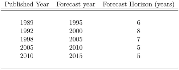
a single year and at a given forecast horizon. Table 1 shows the year of publication
of each report matched with the forecast year for that report; it can be seen that the
forecast horizon varies from five to a maximum of eight years from the publication of
each report. The forecasts for levelised costs used in this paper for a given year were
4
obtained by averaging the costs across EU countries for each technology for the year to
which the forecasts relate. This gives us a single forecast estimate for generation type g
in yearp, which was produced in yearp−h. Thus while country specific evaluations are
desirable when implementing this approach in practice, for this illustrative application
we collapse cross country variation into an EU average for each technology.
[Table 1 here]
We obtained our “contemporary estimates” of levelised costs of energy from Gross
et al. (2013)5. This report provides “contemporary estimates” of the total levelised costs of energy for the technologies identified earlier, but does not provide estimates for
individual cost components such as capital costs, fuel costs, etc. It is for this reason the
analysis which follows is undertaken using levelised costs of energy, rather than individual
cost components. It is worth noting that while Gross et al. (2013) does contain forecast
estimates for the levelised costs of energy, these relate to the post 2010 period for which
we have no “contemporary estimates”, as yet. For some technologies, contemporary
estimates of the LCOE were not available for the forecast year, and so were linearly
interpolated from data for the preceding and following year; again given the illustrative
nature of this empirical exercise this seems a reasonable approach.
The levelised costs for both forecast and contemporary estimates utilised a 10%
discount rate and all currencies were rebased to 2011 GBP using the UK governments
GDP deflators (HM Treasury 2013).
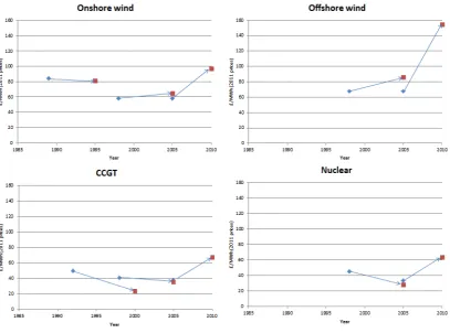
[Figure 1 here]
Figure 1 shows the quantity of data used for the analysis. In all cases, the total
number of paired forecast and actual values for each generation type does not exceed
5
three. Due to this small sample size, the results can only be considered illustrative of
the value of the methodology for assessing the accuracy of forecasts of levelised costs of
energy.
3
Results
3.1 Absolute errors
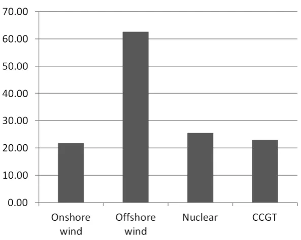
Figure 2 shows the results of the MAE for each generation type across all matched
forecasts and actual values of the levelised cost of energy. As expected, the largest MAE
is for offshore wind technology at greater than £50/MWh6. CCGT and Nuclear have fairly similar errors of around £20/MWh, while onshore wind has the smallest MAE.
Figure 3 shows the RMSE. Only subtle differences can be seen compared to Figure 2.
[Figures 2 and 3 here]
3.2 Percentage errors
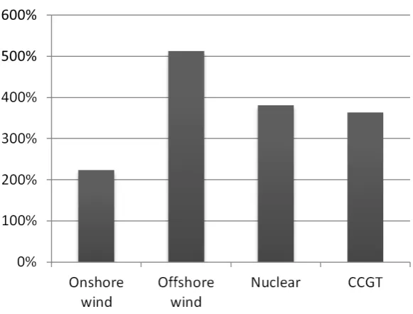
Figure 4 shows the results of the MAPE calculations. The larger observed “errors” are
present for Nuclear and CCGT technologies, while – due to the errors being rescaled by
the absolute value of the LCOE forecast – offshore wind returns a smaller proportionate
error.
[Figure 4 here]
Figure 5 shows the RMSPE for each technology. These results are similar to the
MAPE, however the offshore wind error is larger due to the presence of one larger error.
As already mentioned in Section 2 the RMSPE places greater emphasis on larger, single
errors.
[Figure 5 here]
4
Discussion
4.1 Implications of results
The illustrative results presented in Section 3 reveal that Offshore wind showed the
greatest MAE, RMSE and RMSPE while the MAPE was greater for Nuclear and CCGT.
These results suggest that technologies considered “mature”, such as nuclear and CCGT,
display forecast errors which are higher than both on- and offshore wind in proportionate
terms. The finding that there are also quantifiable MAEs in forecasts of levelised costs of
between£15/MWh and£25/MWh for “mature” technologies like onshore wind, CCGT
and nuclear for a relatively short forecast horizon – one that is far shorter than the
long term typically considered in IAM scenarios – may be important for the range of
sensitivity analysis that can be carried out using IAMs.
Technologies in their infancy typically suffer from an apparent paradox: at this early
stage in the development of the technology, policy makers will place great emphasis
on having cost forecast. Unfortunately, this is when the predictions are often at their
weakest due to a lack of information on the learning rates in the development of these
technologies. It is also possible that past forecast errors will not necessarily be a good
proxy for future errors. One obvious example of this is where there are structural breaks
in key markets, for example with the oil shocks of the 1970s. Such events may lead to
errors estimated using current data to underestimate future forecast errors7.
4.2 Empirical limitations
All of the data used in the illustrative application utilises secondary sources, and was
not collected for the sole purpose of this study. In some years the data suffers from a
lack of data points, and in a few cases relevant contemporary estimates were linearly
7
interpolated from the surrounding years. Overall the total volume of data is not large;
ideally there would be a considerable number of contemporary estimates to match to
more detailed forecasts, with numerous different (and conceivably longer) forecast
hori-zons over which to assess the accuracy of these forecasts of future costs (as presented in
Table 1).
Future empirical applications of these methods are likely to be able to utilise a
more extensive database than we have access to at the moment, in particular access to
proprietary “contemporary estimates” would allow a more detailed comparison of cost
forecasts with realised costs. In particular, analysis of the forecast errors for each of the
components of levelised costs would be an interesting area of future work. However, and
largely for reasons of commercial confidentiality, such data are very difficult to access.
Nevertheless, when using non-proprietary data, it would be desirable to have actual
outturn data.
The only study we are aware of that provides data on the components of the outturn
costs is Koomey & Hultman (2007), in addition to focussing on only one technology and
one country, the data released related to construction projects that took place, in some
cases, up to 35 years before. These data relate only to Nuclear power and only to the
US and as such are not compatible with any of the forecast data that we use here. The
paucity of data on the outturn values of these costs suggests that this is an important
area of future research, particularly given that the IEA produce forecasts of these cost
components.
5
Conclusion and policy implications
This paper has presented a methodology to assess the accuracy of forecasts of costs
of energy. Our methodology requires historical data on forecast and “outturn” costs
range of (short and long-term) forecast horizons. The methodology outlined here was
demonstrated using data on the levelised cost of energy for Nuclear, CCGT and
On-and Offshore Wind, while the methodology could in principle be applied to any forecast
cost which has comparable outturn data.
We find that, in line with expectations, offshore wind forecasts have larger mean
abso-lute errors. Percentage errors proved to be different however; “mature” technologies such
as CCGT and nuclear had the greater errors when compared to wind technologies.
Con-cerns about the data used have been thoroughly addressed, and additional applications
and testing of the methodology with a more comprehensive dataset is recommended.
The data would preferably be primary data, cover a range of energy technologies and be
consistent with forecasts of LCOEs for a range of forecast horizons.
The output of this methodology, in addition to its usefulness in giving some context
to point estimates used by policy-makers, has the potential to improve the output of
analytical work in this area (e.g. using IAMs) by enabling an objective understanding
of the likely range of LCOE forecast errors (or as discussed earlier, for other measures
of costs of energy). More fundamentally, it would be interesting to use the scale of
“errors” from this analysis in applied models like IAMs to understand the importance
of uncertainty surrounding forecasts of technology costs in energy scenarios.
Acknowledgements
Craig Siddons acknowledges funding from the Engineering and Physical Sciences
Re-search Council to the Doctoral Training Centre in Wind Energy Systems, and Grant
Al-lan acknowledges funding from the Scottish Government through the ClimateXChange
programme. The opinions in the paper however are the sole responsibility of the authors
Bibliography
Allan, G. (2011), ‘How wrong were we? The accuracy of the Fraser of Allander
Insti-tutes forecasts of the Scottish economy since 2000’, Fraser Economic Commentary
35(2), 45–53.
Allan, G., Gilmartin, M., McGregor, P. & Swales, K. (2011), ‘Levelised costs of wave
and tidal energy in the UK: Cost competitiveness and the importance of “banded”
Renewables Obligation Certificates’, Energy Policy 39(1), 23–39.
ARUP (2011), ‘Department of Energy and Climate Change Review of the generation
costs and deployment potential of renewable electricity technologies in the UK Study
Report’.
Ashiya, M. (2006), ‘Are 16-month-ahead forecasts useful? a directional analysis of
japanese GDP forecasts’,Journal of Forecasting 25(3), 201–207.
Borenstein, S. (2012), ‘The private and public economies of renewable electricity
gener-ation’, The Journal of Economic Perspectivespp. 67–92.
Edenhofer, O., Hirth, L., Knopf, B., Pahle, M., Schl¨omer, S., Schmid, E. & Ueckerdt, F.
(2013), ‘On the economics of renewable energy sources’, Energy Economics40, S12–
S23.
Granger, C. W. (1996), ‘Can we improve the perceived quality of economic forecasts?’,
Journal of Applied Econometrics11(5), 455–473.
Gross, R., Candelise, C., Heptonstall, P., Greenacre, P., Jones, F. & Castillo, A. C.
(2013), Presenting the Future: An assessment of future costs estimation methodologies
in the electricity generation sector, Technical report, UKERC.
‘Re-newables and the grid: understanding intermittency’, Proceedings of the ICE-Energy
160(1), 31–41.
Grubler, A. (2010), ‘The costs of the french nuclear scale-up: A case of negative learning
by doing’, Energy Policy38(9), 5174–5188.
Harris, G., Heptonstall, P., Gross, R. & Handley, D. (2013), ‘Cost estimates for nuclear
power in the UK’, Energy Policy 62, 431–442.
HM Treasury (2013), ‘GDP deflators at market prices, and money GDP’.
URL:
https://www.gov.uk/government/statistics/gdp-deflators-at-market-prices-and-money-gdp-march-2013
International Energy Agency (1989), Projected costs of generating electricity from power
stations for commissioning in the period 1995-2000, Technical report.
International Energy Agency (1992), Projected Costs of Generating Electricity,
Techni-cal report.
International Energy Agency (1998), Projected Costs of Generating Electricity,
Techni-cal report.
International Energy Agency (2005), Projected Costs of Generating Electricity,
Techni-cal report.
International Energy Agency (2010), Projected Costs of Generating Electricity,
Techni-cal report.
URL:
http://www.oecd-ilibrary.org/energy/projected-costs-of-generating-electricity-2010 9789264084315-en
Koomey, J. & Hultman, N. E. (2007), ‘A reactor-level analysis of busbar costs for US
Krey, V. & Clarke, L. (2011), ‘Role of renewable energy in climate mitigation: a synthesis
of recent scenarios’, Climate Policy11(4), 1131–1158.
Loungani, P. (2001), ‘How accurate are private sector forecasts? cross-country
evi-dence from consensus forecasts of output growth’,International Journal of Forecasting
17(3), 419–432.
Mott Macdonald (2010), ‘UK Electricity Generation Costs Update’, (June).
Mott Macdonald (2011), Costs of low-carbon generation technologies Committee on
Climate Change Costs of low-carbon generation technologies, Technical Report May.
Pons, J. (2000), ‘The accuracy of IMF and OECD forecasts for G7 countries’, Journal
6
Tables
Table 1: Forecast horizons for all data contained within the IEA reports International Energy Agency (1989, 1992, 1998, 2005, 2010).
Published Year Forecast year Forecast Horizon (years)
1989 1995 6
1992 2000 8
1998 2005 7
2005 2010 5
7
Figures
[image:17.595.95.503.139.441.2]Figure 2: MAE by generation technology.
[image:18.595.89.386.414.651.2]Figure 4: MAPE by generation technology.
[image:19.595.90.381.422.643.2]