CUDA accelerated cone‐beam reconstruction

(1)

Theses Thesis/Dissertation Collections

6-1-2011

CUDA accelerated cone‐beam reconstruction

Albert Sze

Follow this and additional works at:http://scholarworks.rit.edu/theses

This Thesis is brought to you for free and open access by the Thesis/Dissertation Collections at RIT Scholar Works. It has been accepted for inclusion in Theses by an authorized administrator of RIT Scholar Works. For more information, please [email protected].

Recommended Citation

(2)

(3)

Thesis

Release

Permission

Form

Rochester Institute of Technology Kate Gleason College of Engineering Title:

CUDA

Accelerated

Cone

‐

Beam

Reconstruction

(4)

DEDICATION

I dedicate this thesis to my parents, for their unending support.

(5)

ACKNOWLEDGMENTS

I would like to thank my committee members Dr. Andreas Savakis for introducing me to

this project and advising me, my supervisor Dr. Jay Schildkraut for his direct cooperation

and support, and Dr. Muhammad Shaaban for being fundamental to my education.

I would also like to thank Rick Tolleson for being the best lab manager, ever.

Lastly, this project would have not been possible without the support of RIT, Carestream

Health, and my family.

(6)

ABSTRACT

CUDA

Accelerated

Cone

‐

Beam

Reconstruction

Albert W. Sze

Supervising Professor: Dr. Andreas Savakis

Cone‐Beam Computed Tomography (CBCT) is an imaging method that reconstructs a 3D

representation of the object from its 2D X‐ray images. It is an important diagnostic tool

in the medical field, especially dentistry. However, most 3D reconstruction algorithms

are computationally intensive and time consuming; this limitation constrains the use of

CBCT.

In recent years, high‐end graphics cards, such as the ones powered by NVIDIA graphics

processing units (GPUs), are able to perform general purpose computation. Due to the

highly parallel nature of the 3D reconstruction algorithms, it is possible to implement

these algorithms on the GPU to reduce the processing time to the level that is practical.

Two of the most popular 3D Cone‐Beam reconstruction algorithms are the Feldkamp‐

Davis‐Kress algorithm (FDK) and the Algebraic Reconstruction Technique (ART). FDK is

(7)

images. However, ART requires significantly more computation. Material ART is a

recently developed algorithm that uses beam‐hardening correction to eliminate

artifacts.

In this thesis, these three algorithms were implemented on the NVIDIA’s CUDA

platform. These CUDA based algorithms were tested on three different graphics cards,

using phantom and real data. The test results show significant speedup when compared

to the CPU software implementation. The speedup is sufficient to allow a moderate

cost personal computer with NVIDIA graphics card to process CBCT images in real‐time.

(8)

TABLES

Note: Tables in the Appendices are not listed here.

Table 1 – GT 330M Specifications ... 40

Table 2 – Summary of Test Plan ... 44

Table 3 – Benchmark Workstation Specifications ... 45

Table 4 – Testing CUDA Graphics Cards Specifications ... 45

Table 5 – Data Sets Description ... 46

Table 6 – Image Comparison for Appendix A ... 51

Table 7 – Images Comparison for Appendix B ... 52

Table 8 – Runtimes for Reconstruction Algorithms ran on CPU & Graphics Cards ... 61

Table 9 – Runtime Scaling for P1, P2, and P3 ... 64

Table 10 – Runtimes for Reconstruction Algorithms ran on CPU & Graphics Cards ... 65

Table 11 – GPU Time Breakdown ... 72

Table 12 – Percentage Breakdown of GPU Time ... 73

(13)

LIST

OF

FIGURES

Note: Figures in the Appendices are not listed here.

Figure 1 – KODAK 9500 Cone‐Beam 3D System [8] ... 2

Figure 2 – Model of How the X‐ray Projection Data is Collected [9] ... 4

Figure 3 – Three Dimensional Coordinate System [1] ... 5

Figure 4 – Parallel Beam Projections [5] ... 6

Figure 5 – Fan Beam Projections [5] ... 7

Figure 6 – The Fourier Slice Theorem [5] ... 8

Figure 7 – CPU Implementation of the FDK Algorithm ... 10

Figure 8 – Object and Projection Representation for ART[5] ... 12

Figure 9 – The Kaczmarz Method, an Iterative Method to Solve a System of Equations [5] ... 13

Figure 10 – CPU Implementation of ART Algorithm ... 15

Figure 11 – CPU Implementation of Material ART Algorithm ... 17

Figure 12 – GeForce 6800 Architecture [10] ... 19

Figure 13 – GeForce 8800 Architecture [11] ... 20

Figure 14 – The Two Streaming Multiprocessors (SM) in a Texture/Processor Cluster (TPC). ... 21

Figure 15 – CUDA Hierarchy of Threads, Blocks, and Grids [12] ... 23

Figure 16 – The Fermi Architecture [12] ... 24

Figure 17 – Streaming Multiprocessor for the Fermi Architecture [12] ... 25

(14)

Figure 19 – Comparison between CPU and GPU in Memory Bandwidth [13] ... 26

Figure 20 – CUDA Implementation of FDK Algorithm ... 33

Figure 21 – CUDA Implementation of ART Algorithm ... 35

Figure 22 – CUDA Implementation of Material ART V1 ... 37

Figure 23 – CUDA Implementation of Material ART V2 ... 38

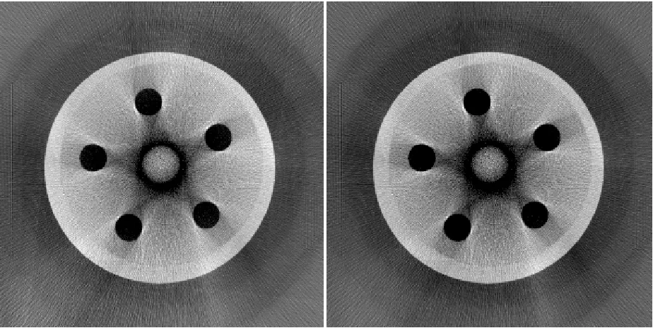
Figure 24 – The Shepp‐Logan Phantom ... 47

Figure 25 – Carestream Health CS 9300 System ... 48

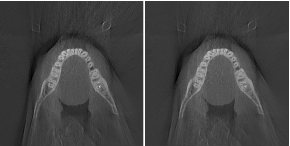
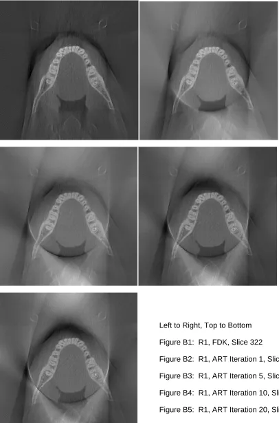
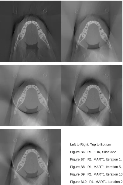
Figure 26 – B1 (R1, FDK, Slice 322) [left]; B5 (R1, ART Iteration 20, Slice 322) [right] ... 53

Figure 27 – B16 (R1, FDK, Slice 364) [left]; B20 (R1, ART Iteration 20, Slice 364) [right] . 54 Figure 28 – Elimination of Vertical Streaking ... 55

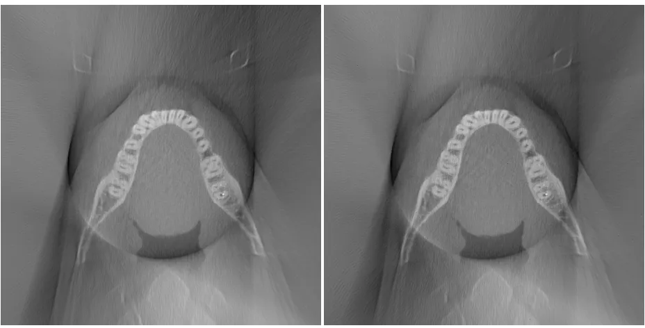
Figure 29 – B25 (R1, MART1 Iteration 20, Slice 364) [left]; B30 (R1, MART2 Iteration 20, Slice 364) [right] ... 56

Figure 30 – Comparison between FDK and ART ... 57

Figure 31 – Comparison between FDK and Material ART V1 ... 58

Figure 32 – Comparison between FDK and Material ART V2 ... 58

Figure 33 – Comparison between Material ART V1 and V2 ... 59

Figure 34 – Truncation Artifact in B31 (R2, FDK, Slice 135) [left]; B35 (R2, ART Iteration 20, Slice 135) [right] ... 59

Figure 35 – Truncation Scenario [22] ... 61

Figure 36 – Reconstruction Algorithms on CPU ... 68

Figure 37 – Reconstruction Algorithms on GTX295 ... 68

(15)

Figure 39 – ART Algorithm Comparison ... 69

Figure 40 – Material ART V2 Algorithm Comparison ... 70

Figure 41 – GPU Time Percentages for ART on Data Sets P1 and P2 ... 75

(16)

LIST

OF

EQUATIONS

Equation 1 – Fourier Slice Theorem [5] ... 7

Equation 2 – Filtered Backprojection [5] ... 8

Equation 3 – The System of Equations for ART[5] ... 12

Equation 4 – Formula to Find the Next Iteration [5] ... 13

(17)

Chapter

1:

Introduction

Computed Tomography (CT) and Cone‐Beam Computed Tomography (CBCT) are two of

many medical imaging technologies that allow doctors and dentists to visualize what is

inside of the human body in three dimensions. Both technologies allow medical

professionals to see all parts of the human body without injuring it.

The main components of Computed Tomography or Cone‐Beam Computed Tomography

are a rotating X‐ray machine and a very powerful digital computer. The X‐ray machine

takes thousands of two‐dimensional “pictures” of the object or the body; digital

computer puts these images together into a highly detailed three‐dimensional image of

what is inside the object. However, 3‐D image reconstruction is computationally

intensive. There are two challenges to computer scientists and engineers: to

reconstruct the 3‐D image in real‐time and to complete it on commodity hardware.

The CBCT scanner is smaller, faster, and safer than the CT scanner. Due to the cone

shaped X‐ray beam, the size of the scanner, amount of X‐rays, and scanning time are

reduced greatly. These can be very beneficial to patients; therefore CBCT scanners are

(18)

Figure 1 – KODAK 9500 Cone‐Beam 3D System [8]

Scientists and engineers have been developing many algorithms to reconstruct 3‐D

images from 2‐D CBCT images. Two of the most popular CBCT algorithms are the

Feldkamp‐Davis‐Kress algorithm (FDK) and the Algebraic Reconstruction Technique

(ART). FDK is the most basic and common reconstruction algorithm. It uses the method

of filtered‐backprojection to reconstruct the original object. FDK is faster than ART but

not as accurate as ART. ART is an iterative method that builds upon the FDK. It uses

projection in conjunction with backprojection to correct for reconstruction artifacts.

Recently developed, Material ART is an improvement over ART, as Material ART will

correct for beam‐hardening. Beam‐hardening is an artifact that occurs when the X‐ray

source is polychromatic. It produces reconstruction artifacts that make the center of

the reconstruction volume denser than it should be. This is because the lower energy

levels get absorbed faster, thus distorting the energy distribution.

(19)

Modern NVIDIA GPUs are scalable processor arrays that excel at computing parallel

tasks. Compute United Device Architecture (CUDA) technology allows general purpose

programs to run on NVIDIA GPUs. Since the reconstruction algorithms are easy to

“parallelize,” image reconstruction of CBCT could be implemented on the CUDA

platform.

The objective of this thesis is to implement three reconstruction algorithms, FDK, ART,

and Material ART, for Cone‐Beam Computed Tomography on NVIDIA GPUs, using CUDA.

Three different NVIDIA GPUs are compared: the high‐end GeForce GTX 560 with 2 GB

graphics memory, the mid‐range GeForce GTX 295 with 1 GB graphics memory, and the

low‐end GeForce G210 with 512 MB graphics memory. These GPUs should provide a

good estimation of the cost‐to‐performance ratio of the CUDA based reconstruction

algorithms.

In the remainder of the thesis, Chapter 2 provides background information on the CBCT

and on the three reconstruction algorithms considered. Chapter 3 describes the

hardware and software architectures of the NVIDIA’s CUDA enabled GPUs. Chapter 4

discusses various implementations of the reconstruction algorithms found in published

scientific papers. Chapter 5 details the implementation of these three algorithms on the

GPU. The test methodology is discussed in Chapter 6, and Chapter 7 reports and

(20)

Chapter

2:

Cone

‐

Beam

Reconstruction

Algorithms

2.1

The

Projection

Model

The model assumed for the collected projection data is that an X‐ray source and

detector plane are rotated about an object. The object could be a patient’s head, as

shown in Figure 2.

Figure 2 – Model of How the X‐ray Projection Data is Collected [9]

Based on this, a coordinate system can be created based on the source, object, the axis

(21)

Figure 3 – Three Dimensional Coordinate System [1]

Figure 3 demonstrates this coordinate system. The reconstruction volume can have an

arbitrary coordinate system, but each projection will have its own detector coordinate

system (illustrated by the u and v axes) and current source location. The source location

will be in volume coordinates. In the implementations, locations are often translated

between these coordinate systems.

2.2

FDK

Algorithm

The FDK algorithm, named after L. A. Feldkamp, L. C. Davis, and J. W. Kress, is one of the

most popular algorithms used for CBCT [4]. It is based on filtered backprojection.

(22)

Figure 4 – Parallel Beam Projections [5]

A projection can be modeled as the line integrals of an object. The diagram at the top

(23)

Figure 5 – Fan Beam Projections [5]

A more accurate model for the projections of X‐rays from a single source is if the lines

form a fan rather than being parallel with respect to each other.

The foundation of tomographic imaging reconstruction is based on the Fourier Slice

Theorem. The Fourier Slice Theorem is:

,

∞

(24)

Where , is the 2‐dimensional Fourier transform of the object and is the

projection of the object at angle . What this means is the Fourier Transform of a

projection is equal to the slice of the object in the frequency domain.

Figure 6 – The Fourier Slice Theorem [5]

Thus, for the case of parallel line projections, the original object can be found through

the polar integral of the weighed (or filtered) inverse Fourier transform of the projection

slices, or:

,

∞

| |

∞

Equation 2 – Filtered Backprojection [5]

Where S w is the Fourier transform at angle θ.

(25)

The case of fan‐beam projections can be derived by reorganizing the projection lines

into the parallel‐line equivalent coordinate system. This introduces another weight into

the formula. The algorithm is completed once it is extended to the 3rd dimension.

Figure 7 gives a high level overview of how the FDK reconstruction works. For each

projection that gets loaded into the program, the projection goes through a Fourier

filter. Then each voxel in the reconstruction object gets modified by backprojection of

the projection data.

The FDK reconstruction has very large amounts of parallelism. Each voxel‐

backprojection operation is independent from each other; therefore, each can run in

parallel. The difference between Figure 7 and Figure 20 shows how a CUDA

(26)

Figure 7 – CPU Implementation of the FDK Algorithm

(27)

2.3

ART

Algorithm

There are three specific computer implementations of algebraic reconstruction

algorithms. They are:

• Algebraic Reconstruction Technique (ART)

• Simultaneous Iterative Reconstructive Technique (SIRT)

• Simultaneous Algebraic Reconstructive Technique (SART)

This thesis implemented SART for CUDA; therefore, we will simply refer to it as ART.

Theoretically, ART approaches the reconstruction in the reverse to FDK. It sets up

systems of equations that describe the reconstruction and uses an iterative method to

reconstruct the original object. Figure 8 and Equation 3 set up the systems of equations,

where N is the number of rays in a projection and M is the number of cells in the object.

Figure 9 and Equation 4 demonstrate the iterative calculations. In practice, the ART is

used to calculate the differences between the currently reconstructed model and the

input projections and uses that to correct any artifacts produced.

(28)

Figure 8 – Object and Projection Representation for ART[5]

(29)

Figure 9 – The Kaczmarz Method, an Iterative Method to Solve a System of Equations [5]

,

·

Equation 4 – Formula to Find the Next Iteration [5]

(30)

The objective is to improve upon FDK. Since ART is an iterative method, it can be

initialized to the FDK reconstruction as the initial guess. Additionally, because ART

needs to converge onto a solution, FDK provides a good initialization; Figure 9

demonstrates this. Therefore, ART is used to produce correction factors upon FDK

reconstruction, to remove the image artifacts and to improve the reconstruction quality.

Figure 10 visualizes ART. The CPU version gives a high level overview of the ART. After

the projection is loaded, the reconstruction object gets forward projected to calculate

what that projection should look like. Then the difference between the projection data

and the forward projection is calculated. This difference is then backprojected onto the

reconstruction object to correct for the difference between the projection data and the

current reconstruction volume.

Similarly to the FDK, the ART has a large amount of parallelism. The backprojection has

the same amount of parallelism compared to the FDK. The forward projection is

detector pixel based, as compared to voxel based backprojection, but it still presents an

(31)

(32)

2.4

Material

ART

Algorithm

A variation of the ART that uses “Material Projection” attempts to correct for beam‐

hardening, a characteristic of X‐rays passing through material. In medical imaging, when

an X‐ray passes through a material, such as flesh or bone, its energy decreases. The FDK

and ART assume that the X‐ray spectrum is either comprised of a single energy level or

comprised of an unchanging distribution of energy levels. However, in real life, neither

is true. As an X‐ray spectrum passes through material, its lower level energies get

absorbed faster than its higher level energies; its energy level distribution changes. This

has the effect of making the interior of the scanned object seem denser than it actually

is and producing additional reconstruction artifacts. This is called beam‐hardening.

Material ART solves this by maintaining an energy distribution count during the forward

projection process, and using it to produce a beam‐hardening correction factor for the

backprojection process. The downside is that it increases the amount of calculations by

the number of energy levels maintained for the forward projection process and another

volume object has to be maintained for the beam‐hardening correction factors. The

beam‐hardening correction factors pose a problem because of the memory costs of

maintaining a large 3D floating‐point volume and the limited amount of memory in

CUDA cards.

The scope of this thesis is to implement CUDA accelerations for all three algorithms.

(33)

Program Start

All 360 degrees

of projections

processed?

Load

projection no

Perform forward

projectionand

calculate image

correction values

Output

reconstruction

object

yes Program End

Backproject

difference onto

voxels and apply

image correction

values

Load FDK

initialization

Max iterations

reached?

no

yes

Calculate difference

between the

projection and the

calculated forward

projection

Note: The new calculations of

Material ART shown in red and

underlined

(34)

Chapter

3:

NVIDIA

CUDA

In 2007, the NVIDIA Corporation introduced the CUDA platform to harness the

computational power of its GPUs. Due to their nature of being large arrays of

processors and their SIMT nature, CUDA can accelerate parallelized computation.

In this chapter, we will review a brief history of the evolution of the GPUs. Next, we

review the G80 “Tesla” architecture and relate it to CUDA. Lastly we discuss the

architectural improvements of the Fermi architecture.

3.1

Brief

History

of

GPUs

The primary purpose of GPUs is to accelerate the computation intensive graphics

pipeline, typically for graphics rendering and video games. The earliest GPUs had fixed

function, but the vertex and fragment stages of the graphics pipeline required the

hardware to become programmable. Also, heavy demand from increasingly

sophisticated video games placed even greater performance demands from GPUs. Early

efforts produced architectures with greater numbers of programmable Vertex and

Fragment processors. However, because graphics workloads were typically unbalanced

between the Vertex and Fragment processors and the increased cost and difficulty in

designing and maintaining two different processors designs, this led to the unified G80

“Tesla” architecture, that was the first CUDA enabled GPU. The subsequent G200 and

(35)

Seperate Vertex processors & Fragment processors

Figure 12 – GeForce 6800 Architecture [10]

Figure 12, Figure 13, Figure 14, Figure 16, and Figure 17 are excerpts from previous

papers that illustrate the evolution of the architecture. Figure 12 visualizes the GeForce

6800 architecture, a typical GPU architecture before the unified architecture; note the

separate discrete vertex and fragment processors. Compare this to the unified

architecture of the GeForce 8800, the first CUDA‐enable GPU. Figure 13 illustrates the

scalable processors array. Figure 16 illustrates the continued evolution and further

improvements made to the architecture; these advancements will be discussed in

(36)

3.2

Main

G80

“Tesla”

Architectural

Features

Figure 13 – GeForce 8800 Architecture [11]

The G80 was the first unified architecture GPU. Instead of the separate vertex and

fragment processors, it is a “Scalable Processor Array (SPA).” This means that they are

comprised of very large arrays of general processing. Figure 13 illustrates the scalable

processor array architecture. Instead of running specialized vertex and fragment

programs or the graphics pipeline, it can run general programs. This is the basis of

CUDA.

(37)

Figure 14 – The Two Streaming Multiprocessors (SM) in a Texture/Processor Cluster (TPC).

Note each SM has 8 Streaming Processors (SP)

The main characteristic of modern GPUs is their parallel nature. They are made of

multiple streaming processors, with each containing eight processing elements called

“CUDA cores.” Figure 11 shows a Texture/Processor Cluster, which contains two

Streaming Multiprocessors (SM). One CUDA core is considered to be a stream

processor, a processor meant to deliver high performance by repeating a set of

instructions or kernel over a batch of data. Another example of a stream processor is

the Cell Broadband Engine Architecture (CBEA).

The CUDA‐enabled GPUs are SIMT in nature, which means Single Instruction, Multiple

Thread. This is similar to SIMD, or Single Instruction, Multiple Data. The difference is

subtle but important. Instead of just simply executing the same set of instructions over

(38)

threads to operate in parallel. Each streaming multiprocessor contains a multithreaded

instruction unit that creates, manages, schedules, and executes threads in groups of 32

parallel threads called warps and manages a pool of 24 warps for a total of 768 threads,

although for CUDA a block is limited to only 512 threads in Compute Capability 1.x.

Because each streaming multiprocessor contains 8 CUDA cores, it makes each streaming

multiprocessor very efficient at processing calculations. Their SIMT nature also makes

the multiprocessor very efficient in utilizing the memory bandwidth and hiding the

latencies. One weakness of the design is that for maximum efficiency, all threads in a

warp must be running the same set of instructions, or divergent threads would occur

and take a performance hit. This also means that the GPU is not very effective at

handling conditional statements, as it lacks the specialized hardware of traditional

processors. Another weakness is that it lacks a unified address space, so it cannot

formally use pointers in the C programming language and any function calls must be in‐

(39)

3.3

NVIDIA

CUDA

Figure 15 – CUDA Hierarchy of Threads, Blocks, and Grids [12]

Compute Unified Device Architecture (CUDA) is the computing engine in NVIDIA GPUs

that allow general programs to run on GPUs. Keeping the G80 Tesla architecture in

mind, it is easy to understand how CUDA takes advantage of the hardware to run

general programs.

It is the programmer’s responsibility to specify explicit parallelism in a program. The

programmer does this by programming a C program to run on the GPU, or a “kernel.”

(40)

organized by blocks, which are organized into a grid. Figure 15 provides a visual

companion for this. Each block of threads corresponds to a SM during execution. The

SM automatically manages the pool of threads in hardware.

3.4

Fermi

Architecture

Figure 16 – The Fermi Architecture [12]

A Streaming Multiprocessor

The Fermi Architecture is the most current architectural leap in NVIDIA GPU design. Its

design improvements include increased CUDA cores per multiprocessor, an increase of

CUDA cores in the GPU overall, a dual‐warp scheduler for each streaming

multiprocessor, a unified address space to support formal pointers, a proper memory

(41)

kernels concurrently. The important feature to note in Figure 16 is the L2 cache (circled

in solid red) and the streaming multiprocessors.

Figure 17 – Streaming Multiprocessor for the Fermi Architecture [12]

Figure 17 is a detailed look at the Streaming Multiprocessor that demonstrates the

greater number of CUDA cores per SM, the L1 cache, and the dual‐warp scheduler and

(42)

Figure 18 – Comparison between CPU and GPU in FLOPs [13]

Half of GTX 295 GTX 560 TI

GTX 560 TI

Figure 19 – Comparison between CPU and GPU in Memory Bandwidth [13]

The end result of the evolutionary pressures on GPU is the current, massive gap in

computational power and memory bandwidth between CPUs and GPUs. Figure 18 and

Figure 19 illustrate this gap.

(43)

Due to its highly parallel nature, it is difficult to predict the performance of a CUDA

program. For example, sometimes the CUDA card has enough streaming

multiprocessors to be able to compute all the blocks at once. Another scenario is that

the CUDA program provides too many blocks at once and some of the blocks have to be

serialized. Then there is yet another consideration that the kernel threads use so little

registers that multiple blocks can run in a single multiprocessor. These factors are

examples of what makes performance prediction difficult.

3.5

Unique

CUDA

Features

Before the Fermi Architecture, NVIDIA GPUs did not have traditional caches to reduce

the effect of access to on‐card memory. Instead, it uses “shared memory.” This is on‐

chip memory that is shared between threads within a block. It operates like a

programmer managed cache, having a read time like a register. Because it is handled by

the programmer rather than automatically handled by the hardware, it is more difficult

to use.

Another unique feature of the GPUs is the texture memory, a cache that stores spatially

local data. It is useful for accessing spatially local data, and it can linearly interpolate

between data points. One disadvantage of texture memory is that, to bind data to

texture memory, the data must either be a simple 1D memory space or an opaque

CUDA array. This means that a separate CUDA array must be allocated each time

(44)

volumes and low amounts of CUDA global memory. Another weakness of texture

memory is that it is read only, which limits its use.

A potential feature for the future is using surface memory. Surface memory can be

written to as well as read from. But this new feature is only available in CUDA Compute

Capability 2.0. Also, it is limited to 2D, not 3D.

Another unique feature to note is constant memory. As the name implies, constant

memory cannot be modified during a CUDA kernel’s runtime. It is stored off‐chip in the

CUDA card’s RAM, but it is cached and optimized for when all the threads in a kernel

access the same memory location simultaneously. There is a pre‐fetch penalty for the

first access, but subsequent accesses only have a latency of one cycle.

Now that all the necessary background material has been sufficiently covered, the next

chapter reviews the previous work on Cone‐Beam Reconstruction Algorithms.

(45)

Chapter

4:

4.1

Algorithms

Medical Imaging Cone‐Beam Reconstruction has been an active topic of research. Due

to its computationally intensive nature, a great deal of effort has been put into creating

more efficient algorithms. The algorithm proposed by L. A. Feldkamp, L. C. Davis, and J.

W. Kress is one of the most popular algorithms used for this field [4]. Cone‐Beam

reconstructions are known to be computationally intensive, so previous research has

focused on acceleration. These efforts include Cone‐Beam Reconstruction

implementations on FPGAs [16][17][18] and on the CBEA (Cell Broadband Engine

Architecture) [14][15]. There has also been work in using GPUs for Cone‐Beam

Reconstruction using shader languages and OpenGL [19][20]. OpenCL is a competing

general purpose GPU (GPGPU) standard, and it has been applied to Cone‐Beam

Reconstruction [21].

4.2

Chapter

5:

CUDA

Implementations

5.1

Overview

One defining characteristic and limitation of all the reconstruction algorithms is the

reconstruction volume size, which, by definition, grows cubically in relation to

reconstruction dimension size. This is the limiting factor when considering what kind of

data sets can be run on the reconstruction programs. Simply put, a CUDA card cannot

run a program that requires more device RAM than what the card has. Typically this is a

problem for reconstruction volumes.

Another characteristic that is common for all CUDA implementations is that they all use

constant memory for the kernel parameters. One challenge is that due to the

complexity of the kernels, a very large number of parameters were needed. Putting

them into the parameter list of the kernels would increase the number of registers used

and is likely to cause the use of shared memory. Constant memory is a way around that.

This is also one of the tips included in the CUDA Best Practices [23].

5.2

Important

Points

about

CUDA

There are a number of possible bottlenecks that can severely reduce parallel

computation and performance gains. Often, these are memory bottlenecks. CUDA’s

extreme parallel nature often turns compute bound problems into I/O bound problems.

(48)

The first bottleneck is the memory transfer between the CUDA device and the host

system. This is usually the largest bottleneck, because CUDA cards have a limited

amount of DRAM/global memory and the PCI‐Express bus is the slowest component

between the host system and the CUDA device.

The second bottleneck is the Global memory access. Just like in conventional computer

systems, accesses to RAM are extremely costly. For CUDA, accesses to the global

memory cost hundreds of cycles in latency. CUDA uses the multiple warps in a block to

attempt to hide the latency, but optimization typically involves reducing Global memory

accesses. Other types of memory such as texture memory, constant memory, and

shared memory can be used. Compute capability CUDA 2.0 made the architectural

improvement of formal caches, so it reduces the penalty of Global memory accesses.

5.3

CUDA

Accelerated

FDK

As discussed previously, FDK is based on filtered backprojection. This means FDK can be

(49)

(50)

Fourier filtering is implemented by using the Fourier transform to transform the

individual rows of the detector image, multiplying the Fourier signal with the filter, then

performing the reverse transformation to get back the filtered signal. CUDA already has

an implementation of Fast Fourier Transformation in its SDK, called the CUFFT. A simple

signal multiplying kernel and the CUFFT are used to implement the CUDA version of

Fourier filtering.

The backprojection is a relatively straight port from the original C++ code. As discussed

previously, the code was parallelized along individual voxels. In detail, each voxel would

calculate the direction of their X‐ray and use that to calculate where it would hit the

detector. Then the kernel would use the built‐in bilinear interpolation in the texture

memory. This feature is important for a couple of reasons: it is a built‐in function so it

reduces the demand for registers and CUDA cores and it reduces Global memory

accesses because the texture memory is cached for spatially localized data.

An attempted version of FDK was the “reworked FDK.” This was developed in an effort

to achieve the same speedup that was seen in [1]. It achieved greater efficiency by

loading all the projection data to the CUDA card in the beginning, and running one

kernel for all projections instead of one kernel run for each projection. This was

discontinued because it could only work for data set with 360 projections (due to the

use of constant memory) and thus it was less flexible. And even though it resulted in a

(51)

5.4

CUDA

Accelerated

ART

All 360 degrees

of projections

processed?

Load

projection no

Calculate difference

between projection

and calculated

forward projection

Output

reconstruction

object

Program End

CUDA:

Backproject

difference onto

voxel (0,0,0)

CUDA:

Backproject

difference onto

voxel (0,0,1)

CUDA:

Backproject

difference onto

voxel (x,y,z) ...

CUDA:

Backproject

difference onto

voxel (0,0,2)

CUDA:

Read

reconstruction

object from

CUDA device

yes

Program Start

Max iterations

reached?

no yes

Load FDK

initialization

CUDA:

Load FDK

initialization

onto CUDA

device

CUDA:

Forward project

reconstruction data

onto pixel (0,0)

CUDA:

Forward project

reconstruction data

onto pixel (0,1)

CUDA:

Forward project

reconstruction data

onto pixel (x,y) ...

CUDA:

Forward project

reconstruction data

onto pixel (0,2)

CUDA:

Load

difference

onto CUDA

device

(52)

Remember that ART is the theoretical opposite of FDK. As it has been discussed in

previous literature [15], using Forward Projection to correct for backprojection, or

implementing SART, has been shown to be effective in reducing and eliminating

reconstruction artifacts, increasing image sharpness, and increasing overall

reconstruction quality.

Forward projection works by calculating the direction of the X‐ray for each pixel of the

detector, and using ray casting to calculate the attenuation value of that detector pixel.

Then the backprojection step uses the difference between the input projection data and

the calculated projection data to correct for any differences found between them.

Similar to using texture memory for the 2D detector data, forward projection uses a 3D

texture for the reconstruction data. This is done for the same reasons. Unfortunately,

due to the previously mentioned reconstruction volume size problem and for CUDA

cards with low amounts of global memory, a problem becomes apparent. For the

typical reconstruction size of 5123, a 1 GB CUDA card cannot maintain both the normal

reconstruction volume and the CUDA array reconstruction volume that is bound to the

texture memory at the same time. What happens then is that the volume has to be

copied back to the host each time for the backprojection step. This is not a major

problem for reconstruction sizes of 2563, but the memory transfer takes up far more

(53)

5.5

CUDA

Accelerated

Material

ART

(54)

Figure 23 – CUDA Implementation of Material ART V2

Adds a "merged kernel" (in red

and underlined)

Material‐ART has its own unique challenges. The Image Correction Factors volume, by

definition, is the same size as the reconstruction object. The typical case size for

reconstruction volumes is 5123 floating point values, or 512 MB. However, the typical

CUDA card only has less than 1 GB of RAM. This would make it impossible to maintain

both the reconstruction volume and the image correction volume in memory at the

(55)

RAM. The second solution is to modify the implementation of the algorithm, or make

minor changes to the algorithm itself to eliminate the need to maintain the Image

Correction Factors in the main memory. This second solution can be implemented by

recalculating the Image Correction Factors on the fly for the reconstruction step. This

modification becomes the basis of the “merged kernel” implementation. The merged

kernel ray casts from the detector pixel just like the forward projection step, and

calculates and applies the image correction values. The merged kernel is separate from

the forward projection and back projection, as shown in Figure 23. The disadvantage of

this method is the increase in calculation and possible synchronization errors.

There are further notes on the implementation of Material ART. As mentioned before,

Material ART is more complex and requires more computation. It also requires

additional parameters. This is because during the forward projection step, at the

section when Material ART reads from the reconstruction volume, it takes the

attenuation of the voxels and classifies them to materials from a materials list received

in the parameters. This means that a material ART program would require both a

Materials list and the expected attenuation values for the expected materials. The

attenuation values come from the National Institute of Standards and Technology.

Ideally, the energy levels per detector pixel and the additional parameters for Material

ART should be placed in shared memory. However, they were not. The primary reason

(56)

would take up, and there is a limited amount of memory space of shared memory per

each block. Additionally, energy levels must be maintained per ray casted. Because a

large amount of threads were grouped per block and the energy spectrum can be

divided into an arbitrary number of levels, the memory requirements would exceed

shared memory capacity. These reasons combined with the difficulty of developing in

CUDA and the generous amount of space in global memory, these additional

parameters were delegated to global memory. The cache of the Fermi architecture

makes this debate moot, as the cache effectively eliminates the global memory penalty.

One potential source of error is that the actual energy levels of the X‐ray sources are not

known; since proper calibrations were not done. The energy levels provided for the real

data reconstructions are estimates. Even if copper was used to filter the X‐ray source,

the X‐ray source is still polychromatic.

5.6

Development

Development of the CUDA accelerations was done on a TOSHIBA Satellite A665‐S6050

Laptop with a GT 330M. The specifications are below:

Table 1 – GT 330M Specifications

Graphics

Card

Compute

Capability

Number of

multiprocessors

Number of

CUDA cores RAM GFLOPS

GT 330M 1.2 6 48 1GB 182

As running typical size data sets (5123 reconstruction dimensions) was time consuming

(57)

dimensions) instead, with the assumption that the runtime characteristics remain the

same.

In implementation, data transfers between the host and device and global memory

accesses were minimized. There are only two exceptions:

1. Because in‐development profiling indicated that calculation dominated GPU

time, so texture memory was utilized to reduce global memory accesses and

overall kernel time. This comes at the cost of increased memory transfers

between the host and device. More details are discussed in the analysis of

section 7.3.3 ART and Material ART and section 7.3.4 GPU time breakdown.

2. The size of Material ART parameters are not constant and are not

guaranteed to keep the same dimensions. Due to these reasons and the low

amount of available shared memory, the parameters were placed in global

memory.

5.6.1

ART

vs.

Material

ART

ART implements the use of texture memory to both calculate the bilinear and trilinear

interpolation and to cache the memory accesses. The Material ART cannot use the

interpolation of the texture memory, because it has to classify the accessed voxels

before calculating the effective attenuation value. This was considered to be a

disadvantage with an expected effect of slower kernel execution due to increased global

(58)

in global memory as stated before, so the additional global memory accesses are

expected to reduce kernel execution performance.

5.6.1.1 Memory Swapping

By necessity of using the texture memory and the size of the typical usage case, the

reconstruction volume has to be swapped between the system and the CUDA card. As

previously mentioned, the typical dimension size is 5123 or 512 MB and the older CUDA

cards only have 1 GB of memory.

The typical steps of runtime case are:

1. Allocate 3D CUDA array for reconstruction volume

2. Bind 3D CUDA array to texture memory

3. Execute Forward Projection Kernel

4. Free CUDA array

5. Allocate 3D memory space for Backprojection

6. Copy over the reconstruction volume from the system to the CUDA device

7. Execute the Backprojection Kernel

8. Copy back the reconstruction volume from the CUDA device

9. Free the 3D memory space

10. Go back to step 1 if it is not the final projection and iteration

The problem is that because of the limited RAM in the CUDA card, it is not possible to

(59)

need for swapping. Material ART is different because it allocates the 3D volume at the

start and maintains it throughout the entire runtime, it does not swap the volume.

In‐developing profiling shows that the swapping of a 2563 volume does not significantly

impact runtime. More information on this is presented in the results and analysis of

section 7.3.3 ‐‐ ART and Material ART and section 7.3.4 ‐‐ GPU time breakdown.

The next chapter discusses the test to confirm the CUDA implementation of the

algorithm.

(60)

Chapter

6:

Test

Methodology

Table 2 – Summary of Test Plan

CPU G210 GTX295 GTX560

P1 headphantomTiny FDK, ART,

MART1, MART2

FDK, ART, MART1, MART2

P2 headphantomTiny FDK, ART,

MART1, MART2

FDK, ART, MART1, MART2

P3 headphantomTiny FDK, ART, MART2

P4 hardeningphantom FDK, ART, MART2

R1 9300_Patient_321 FDK, ART, MART2

R2 9300_Patient_349 FDK, ART, MART2

R3 Bacelone_head_R23

R4 Rod_corticalbone FDK, ART,

MART1, MART2

FDK, ART, MART1, MART2 Hardwares / Algorithms to be tested

Dataset Actual Name Data Source Remarks

All 1 iteration

All 1 iteration. GTX295 to run 20 iterations on ART, MART1, & MART2 FDK, ART,

MART1, MART2 Computer

generated

CBCT Data

FDK, ART, MART

Testing and benchmarking was completed across three graphic cards and eight data sets

on a workstation that can support all three graphics cards. Table 2 provides a summary

of the test plan. It will be covered in further detail in the following sections. The

workstation is a Windows XP SP3 system with an AMD Athlon 64 X2 Dual Core 5600+

processor. Further details are shown in Table 3.

(61)

Table 3 – Benchmark Workstation Specifications

System Information

Operating System Windows XP Professional SP3 System Manufacturer Gigabyte Technology Co., Ltd.

System Model GA‐MA790X‐DS4

Processor AMD Athlon(tm) 64 X2 Dual Core Processor 5600+, MMX, 3DNow (2 CPUs), ~2.9GHz

Memory 2814MB RAM

PCI Express 2.0 x16 2

Power Supply Antec True Power Trio TP3‐650 650W Power Supply with Three 12V Rails

6.1

CUDA

Graphics

Cards

Three CUDA cards were selected to test the performance and behavior of the CUDA

programs across different CUDA cards. These cards are:

Table 4 – Testing CUDA Graphics Cards Specifications

card name compute capability

Number of

multiprocessors

Number of

CUDA cores RAM GFLOPS

G210 1.2 2 16 512MB 69

GTX 295 1.3 2x30 2x240 2x1GB 2x894

GTX 560 2.1 8 384 2GB 1263

Three CUDA graphics cards, G210, GTX 295, and GTX 560, were used to test the

performance and behavior of the reconstruction algorithms on CUDA. At present, G210

is a low‐end graphics card with 512 MB graphics memory, GTX 295 is a mid‐range card

with 1 GB graphics memory, and GTX 560 is a high‐end card with 2 GB graphics memory.

They have different amounts of memory in order to demonstrate the memory limit on

the reconstruction algorithms. The GTX 560 has Compute Capability 2.0, compared to

(62)

architectural improvements. The GTX 295 is different from others in that it combines

two physical NVIDIA GPUs into one graphic card. However, this thesis’ CUDA

implementation of reconstruction algorithms only utilized one GPU because

programming of two GPUs is beyond the scope of this thesis. The CUDA card used for

development, the GT 330M, is closer to the G210 rather than the GTX 295.

6.2

Data

Sets

Table 5 – Data Sets Description

Column Row Size (KB) Problem

Size (MB) Column Row Slice Size (MB)

Problem

Size (GB)

P1 360 128 128 64 23 128 128 128 8 3 P2 360 256 256 256 90 256 256 256 64 23 P3 360 512 512 1024 360 512 512 512 512 180 P4 360 512 512 1024 360 512 512 512 512 180 R1 246 575 640 1438 345 576 576 450 570 137 R2 449 960 768 2880 1263 576 576 450 570 250 R3 360 600 950 2227 783 608 608 608 857 301 R4 360 600 950 2227 783 300 300 200 69 24

Detector Volume No. of

Projections Dataset

Eight data sets, provided by Carestream Health, Inc., were used for testing. They are

divided between computer generated data and real data. The real data refers to

projection data produced from CT scans of patients and phantoms. Computer

generated data are not produced from X‐ray machines. The real data are further

distinguished between the patients and phantoms. Phantoms are manufactured objects

that test reconstruction algorithms. A well known and commonly used phantom is the

Shepp‐Logan Phantom. Figure 24 shows the Shepp‐Logan Phantom. Computer

(63)

Figure 24 – The Shepp‐Logan Phantom

Two types of phantoms were used for the computer generated data: the standard

phantom and the Material‐phantom, a phantom specifically used to test cone‐beam

correction. Also, because they are generated, different sizes of these phantoms will be

used. For real data, CT‐scans of patients were used as the final test and benchmark to

verify that the algorithms work, and that the ART and Material‐ART improve

reconstruction quality. Also, CT data of a real phantom was used to detect beam‐

hardening correction. Four sets of real data were used. Two data sets were selected to

have manageable dimensions, while the third was selected because its dimensions are

too large for the program to handle; these data sets were selected to verify the

memory‐bound problem.

(64)

Figure 25 – Carestream Health CS 9300 System

The real data sets R1 and R2 were scanned in the CS 9300 system, while the real data

set R3 was scanned in the KODAK 9500 Cone Beam 3D System. The real data set R4 was

scanned in an unspecified scanner.

The real data sets were used to test for image quality. Visual inspection was used to

determine image quality; the results from multiple programs running on the same data

set were compared. The FDK results served as the baseline, as it has the fastest runtime

but the poorest image quality. The FDK results were compared to the ART and Material

ART results. Between the FDK and ART results, specific details were examined, such as

image sharpness of image details and the correction of artifacts. Within the ART and

Material ART, the image qualities between different numbers of iterations were

compared to find the number of iterations needed to produce optimal image quality.

(65)

The results of the two Material ART implementations were compared to confirm the

validity of the alternate Material Art implementation and to make sure the second

Material ART implementation did not produce additional artifacts.

6.3

Expected

Results

Before benchmarking was performed, there were a number of expectations for the

results. These expectations are as follows:

• The newer GPU should have faster runtimes than the older ones.

• FDK will be the fastest algorithm, followed by ART, Material ART V1, and

Material ART V2.

• The main limitation of what data sets can be run on which CUDA cards will be

dictated by the amount of RAM the CUDA card has. It is expected that the G210

can only run the smallest reconstruction sizes (P1, P2, and R4) since it has only

512 MB of RAM. GTX 295 is expected to be able to run almost all of the cases

except R3 due to its extremely large reconstruction size.

There are additional expectations for Material ART. Because the real data sets R1, R2,

and R3 have their source filtered through copper, they effectively have minimal beam‐

hardening; Material ART will not produce a significant difference compared to the ART

results. This is why R4 was selected to confirm beam‐hardening.

All the necessary data was collected by following this test plan. The next chapter

(66)

Chapter

7:

Results

and

Analysis

7.1

Image

Quality

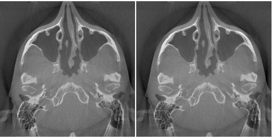
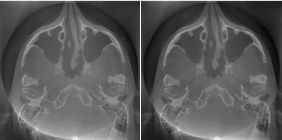
The real data sets R1, R2, and R3 are CT scans of patient’s heads. Of these, the features

of interest are the molars, molar implants (e.g., dental fillings), sinus bones, and ear

bones. The reconstruction slices are shown because they either have a feature of

interest or they showcase the elimination of an artifact. R4 is a slab of acrylic with six

rods of bone‐like material. It was made to be the same as the Hardening Phantom P4.

The first criterion for the results of the CUDA accelerations is the image quality of the

output. As stated by the proposed testing, there are several points that have to be

confirmed. These are:

1) Confirm that the GPU produces images that are the same quality or better

quality compared to the CPU output

2) Confirm the quality improvement of ART over FDK and determine how many

iterations are needed

3) Confirm that Material ART confirms beam‐hardening

4) Confirm Material ART V2 produces the same output images as Material ART V1

Because there are a very large number of images to be presented, the images are placed

(67)

inspection; what we are interested in is the removal of image artifacts and overall

increase in image quality.

7.1.1

GPU

vs.

CPU

Table 6 – Image Comparison for Appendix A

CPU GTX560

R1 FDK 322 A1

=

A2

R1 ART 322 A3

<

A4

R1 MART1 322 A5

=

A6

R1 MART2 322 A7

=

A8

R2 FDK 135 A9

=

A10

R2 ART 135 A11

<

A12

R2 MART1 135 A13

=

A14

R2 MART2 135 A15

=

A16

R4 FDK 38 A17

=

A18

R4 ART 38 A19

<

A20

R4 MART1 38 A21

=

A22

R4 MART2 38 A23

=

A24

= Images are similar per visual comparison

< GPU Image is better than CPU Image per visual comparison

Dataset Algorithm Image

Slice

Image Comparsion

Visual

Image

Comparison

on

Reconstruction

Algorithms

Ran

on

CPU

&

GTX560

Appendix A contains selected slices of the reconstructed volumes for the real data sets.

The CPU results are on the left side. The GPU results are on the right side. The point of

(68)

the same output or of better quality than images of CPU implementations. Through

visual inspection, we can confirm this is true.

7.1.2

ART

vs.

FDK

Table 7 – Images Comparison for Appendix B

R1 ART 322 B1 << B2 << B3 << B4 < B5

R1 MART1 322 B6 << B7 << B8 << B9 < B10

R1 MART2 322 B11 << B12 << B13 << B14 < B15

R1 ART 364 B16 << B17 << B18 << B19 < B20

R1 MART1 364 B21 << B22 << B23 << B24 < B25

R1 MART2 364 B26 << B27 << B28 << B29 < B30

R2 ART 135 B31 << B32 << B33 << B34 < B35

R2 ART 190 B36 << B37 << B38 << B39 < B40

R3 ART 443 B41 << B42 << B43 << B44 < B45

R3 ART 527 B46 << B47 << B48 << B49 < B50

R4 ART 38 B51 << B52 << B53 << B54 <

CUDA accelerated cone‐beam reconstruction