An experimental study of unsteady hydrodynamics of a single scull

http://pim.sagepub.com/

the Maritime Environment

Engineers, Part M: Journal of Engineering for

http://pim.sagepub.com/content/early/2011/06/10/1475090211406775

The online version of this article can be found at:

DOI: 10.1177/1475090211406775

published online 14 June 2011

Proceedings of the Institution of Mechanical Engineers, Part M: Journal of Engineering for the Maritime Environment

A H Day, I Campbell, D Clelland and J Cichowicz

An experimental study of unsteady hydrodynamics of a single scull

Published by:

http://www.sagepublications.com

On behalf of:

Institution of Mechanical Engineers

can be found at: Maritime Environment

Proceedings of the Institution of Mechanical Engineers, Part M: Journal of Engineering for the Additional services and information for

http://pim.sagepub.com/cgi/alerts

Email Alerts:

http://pim.sagepub.com/subscriptions

Subscriptions:

http://www.sagepub.com/journalsReprints.nav

Reprints:

http://www.sagepub.com/journalsPermissions.nav

An experimental study of unsteady hydrodynamics

of a single scull

A H Day1*, I Campbell2, D Clelland1,andJ Cichowicz1

1

Department of Naval Architecture and Marine Engineering, University of Strathclyde, UK

2

Wolfson Unit for Marine Technology and Industrial Aerodynamics, University of Southampton, UK

The manuscript was received on 18 January 2011 and was accepted after revision for publication on 22 March 2011.

DOI: 10.1177/1475090211406775

Abstract: The effect of hull dynamics on the hydrodynamic performance of a single scull is investigated via a combination of field trials and tank tests. The location of laminar-turbulent transition in unsteady flow is explored via several series of hot-film measurements on the bow of a full-scale single scull in unsteady flow in both towing tank and field-trial conditions. Results demonstrate that the measured real-world viscous-flow behaviour can be successfully reproduced in the tank using an oscillating sub-carriage to reproduce the surging motion mea-sured in the field trials. It can be seen that there is a strong link between turbulence and accel-eration; results show that the link is relatively insensitive to mean velocity, but that small changes in acceleration time-histories can have a marked effect, as can the presence of small waves.

The impact of the location of laminar turbulent transition is investigated by way of a series of resistance tests, both with free transition and with transition forced by turbulence stimula-tion at two different locastimula-tions. Results indicate that an aft movement of 200 mm of the loca-tion of transiloca-tion can reduce resistance by almost 0.5 per cent. Unsteady tests using the oscillating sub-carriage indicate that unsteady effects add around 3 per cent to the total mean resistance with free transition.

Keywords:hydrodynamics, rowing, hull resistance, boundary-layer transition, tank tests, field trials, unsteady speed

1 INTRODUCTION

1.1 Background and literature review

Sailing has led the way for many years in boat-based sports in the application of performance assessment techniques at the design stage. Physical testing – in towing tanks, wind tunnels, and at full-scale – is widely used in tandem with computational analysis,

driven especially by the high budgets of America’s Cup yacht design. In contrast, the use of both com-putational hydrodynamics and physical testing in performance assessment of hulls for rowing, canoe-ing, and kayaking has been more limited.

Nonetheless, the extremely small winning mar-gins in rowing justify the extraction of every last possible improvement, encouraging the possibility of performance improvements through hull design optimization. In the Beijing Olympics, 18 crews over the 14 rowing events were within 0.5 per cent of mean speed of the gold medal-winning crews in their event, from as low as fourth place, while 33 were within 1 per cent.

A limited number of computational studies of rowing shells have been carried out using a range of tools, from inviscid slender-body and thin-ship

*Corresponding author: Department of Naval Architecture and Marine Engineering, Universities of Glasgow and Strathclyde, Glasgow G4 0LZ, UK.

email: [email protected]

codes through to viscous computational fluid dynamics (CFD), predominantly using steady-speed approaches. Scragg and Nelson [1] used a steady-speed thin-ship wave-resistance code, including shallow-water effects, to predict rowing shell perfor-mance and design a series of hulls, two of which were subsequently constructed and tank-tested. Tuck and Lazauskas [2], and Lazauskas [3] used a steady-speed thin-ship approach to study optimal shapes for rowing shells. Formaggia et al. [4] com-puted the effects of heave and pitch motions on resistance using a potential-flow approach; Formaggia et al. [5] utilized this in a sophisticated dynamic model of the rower–hull–fluid system. Berton et al.[6] presented results for a one-degree-of-freedom unsteady viscous CFD approach for a rowing shell.

Other studies (e.g. Wellicome [7]) have utilized steady-speed tank tests as an aid to the develop-ment of improved hull-forms for rowing shells; many other tank-test studies carried out remain commercially confidential. Published data from tests with unsteady speed are few and far between. Doctorset al. [8] tank-tested a benchmark ‘Wigley’ hull with sinusoidally varying speed in deep and shallow water, and compared their results with an unsteady thin-ship code. With low-frequency oscillations, some large unsteady wave-making effects were observed, especially in shallow water; these were successfully predicted by the unsteady code developed. However, results were not pre-sented for higher frequency oscillations more rele-vant to rowing. In one of the only published studies including experiment measurement of unsteady speed on rowing shells, Scragg and Nelson [1] carried out resistance tests on one-third-scale models of two eights designed using their numerical study alongside a benchmark hull, including some tests involving pitching and sur-ging; however, the details of the motions involved are not clarified.

The acceleration and velocity variation of a row-ing shell in surge can be substantial. Kleshnev [9] measured the surge acceleration for a men’s rowing pair at a rate of 35 strokes/min; in the ‘catch’ phase of the stroke, the peak deceleration was over 1 g. The associated range of speed variation, assuming a mean speed of 5.0 m/s (equivalent to a medal time for a rowing pair in Beijing) is almost 50 per cent of the mean value; in 3.0 m water depth, typical of man-made rowing lakes, the depth Froude number would vary from 0.65 to 1.09.

The resistance is modified in two key ways by the variation in speed. The development of the bound-ary layer around the hull will be affected, leading to

changes in the viscous resistance; these changes are likely to be relatively insensitive to water depth. Second, the waves generated by the boat, and the associated wave-making resistance, will change; the effect of unsteady speed on wave-making will be more pronounced in shallow water, especially close to the critical depth Froude number of 1.0.

One parameter of boundary layer behaviour known to be of particular practical relevance in yacht hull design is the location of laminar–turbu-lent transition; designing to delay transition is a key strategy for resistance reduction in yachts, and con-sequently the determination of transition location and the intermittency of turbulence has been inves-tigated in detail by America’s Cup technical teams through tank tests and field trials (e.g. Binns et al.

[10]).

1.2 Aim and objectives

The current study aims to explore the effect of unsteady hull dynamics on the hydrodynamics of rowing shells, with particular emphasis on the development of the boundary layer near the bow, and the impact of the unsteady velocity on the hull resistance.

The objectives of the current study are:

(a) to examine the impact of unsteady speed on boundary layer transition around the hull in real-world rowing conditions;

(b) to reproduce the velocity profiles measures in field trials in the towing tank using an oscillat-ing sub-carriage and to examine the extent to which the boundary layer behaviour can be modelled in test tank conditions;

(c) to use tank-test data to explore the key para-meters in determining the impact of unsteady speed on boundary layer transition around the hull;

(d) to explore the impact of unsteady speed on resistance via tank tests.

2 MEASUREMENT OF UNSTEADY BOUNDARY-LAYER TRANSITION

2.1 Field trials

The field trials carried out had two key objectives: first to measure realistic speed profiles for reproduction in the tank, and second to provide field measurements of boundary-layer transition in the presence of fully realistic hull motions and levels of background turbu-lence for comparisons with test-tank data.

Three series of field trials were carried out, in varying conditions and locations in the South of England, allowing progressive refinement of the measurement procedures, and also allowing the rower to become accustomed to the reduced stability of the hull resulting from the installed equipment. The scull was fitted with conventional hot-film anemometry gauges in a number of differ-ent locations. The first series was treated simply as a commissioning trial to check that the instrumenta-tion worked and that the stability of the scull was adequate. In the second series several gauges were set up on each side of the hull to explore behaviour at different locations on the hull. In each run the forward gauges only were logged; the scull was then brought ashore, and the forward gauges removed to allow undisturbed flow to the next set of gauges fur-ther aft. This allowed the positions of most interest to be identified, which were then adopted in the tank tests. In the third and final series of tests one gauge was located on each side in the positions identified to capture a larger data set for compari-son with tank tests.

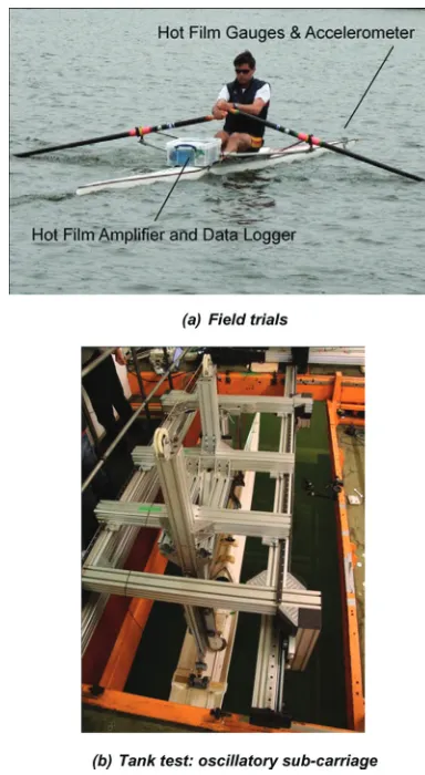
An integrated system designed for logging race-car data was employed in this study. The system comprises a global positioning system (GPS) to cap-ture mean speed, accelerometers to obtain surge and pitch motions, and a portable data logger including analogue inputs used here to gather the hot-film data. The data logger, hot-film amplifiers, and batteries were mounted in a waterproof box, aft of the foot stretcher, as shown in Fig. 1(a).

Several runs were made during each series of trials; each run included some ‘cruising’ strokes, some ‘racing’ strokes, and also a ‘coast-down’ period, in which the scull decelerates smoothly in a natural manner.

2.2 Tank tests

The tank tests were carried out in the towing tank at the Kelvin Hydrodynamics Laboratory in Glasgow, Scotland, using a scull which was similar, but not identical to that used in the field trials. Unfortunately, logistical and budgetary constraints precluded the use of a scull identical to that used in the field trials; however, as the results will show, the hydrodynamic behaviour with regard to

laminar–turbulent transition is generally very simi-lar between field trials and tank tests. The lines plan of the scull was measured up to a point around 25 mm below the deck edge; the body plan is shown in Fig. 2 and the details of the hull are shown in Table 1. It can be seen that the bow, shown on the right of Fig. 2 exhibits more V-shaped sections than the stern (on the left). Tank tests were carried out between the second and third set of field trials.

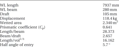
The tank has dimensions 76.034.5732.5 m; water depth was set at 2.15 m for these tests. The water depth is therefore less than that which would be expected in a rowing event; this will have some impact on the wave-making resistance (see section 4), but is unlikely to have any significant impact on the viscous flow phenomena, including transition. The mean speed was generated by the main towing carriage; a sub-carriage, shown in Fig. 1(b), gener-ated the surging motion. The sub-carriage is pow-ered by a digitally controlled, electrically driven actuator, with maximum travel of 1 m, speed of 2 m/s, acceleration of 20 m/s2, and force of 20 kN. The standard towing system is mounted on the sub-carriage.

Pre-calculated data points specify carriage posi-tion at each moment through one cycle; the cycle is repeated to generate periodic motion. More com-plex carriage trajectories can be created in order to simulate non-periodic motion, such as acceleration from the start, by synchronizing the sub-carriage and main carriage drives, although this was not attempted in the current study.

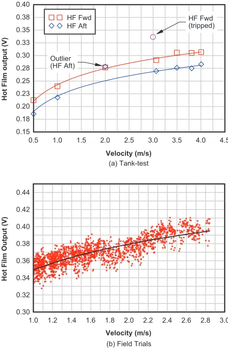
In this study the trajectory data were obtained from the second set of field trials. The carriage tra-jectory is started from a point of zero sub-carriage velocity, when the instantaneous scull velocity is equal to its mean value and the carriage excursion is at one extreme. However, the mean velocity varies slightly from stroke to stroke; thus if the end point is chosen to give the same total velocity as the start point, then the net motion of the carriage may not be zero over the cycle. Some slight adjustment of the trajectory is then required in order to ensure that the net motion is exactly zero, to avoid the sub-carriage creeping down the rails during the tests. The trajectory adopted for a fast rowing stroke, with period 1.84 s, is shown in Fig. 3; phases of the stroke are labelled following Kleshnev [9]. Here the start and finish of the stroke is referenced to the local

peak in acceleration just prior to the catch, which corresponds approximately to the zero position of the carriage excursion.

In reality, as well as surging, the boat pitches through the stroke cycle owing to both the fore-and-aft movement of the athlete and the surging accel-eration, while vertical acceleration of the athletes and oars leads to a heaving motion. In the current system the surge motion is controlled, but the scull can heave and pitch freely owing to the varying hydrodynamic forces. Consequently some compo-nents of pitch and heave are not modelled correctly in these tests; however, examination of video sug-gests that vertical bow motions are represented rea-sonably realistically.

Hot-film gauges were applied in positions simi-lar to those used in the final set of field trials; sig-nals were processed using the same amplifier as adopted for field trials and logged on a 16-bit ana-logue to digital converter. The gauge locations were 400 mm and 600 mm aft of the forward extent of the bow; this corresponds to 275 mm and 475 mm aft of the forward extent of the waterline with the crew weight approximately at the mid-position of the seat travel.

3 TEST RESULTS

3.1 Non-oscillatory runs

A series of tank runs were carried out at steady speed to test and to calibrate the hot-film measure-ments. Data were filtered with a 20 Hz low-pass digital filter to remove electrical noise. Figure 4 shows a time history of a typical run.

Hot-film signals can be characterized as consist-ing of four main components: a DC signal which

Fig. 2 Body plan of single scull tested in tank

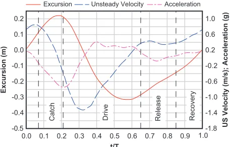
Table 1 Principal dimensions and coefficients of scull tested

WL length 7937 mm

WL beam 280 mm

Draft 105 mm

Displacement 118.4 kg

Wetted area 2.340 m2

Prismatic coefficient (Cp) 0.641

Length/beam 28.373

Beam/draft 2.657

Length/vol1/3 _16.162

Half angle of entry 5.7°

varies non-linearly with speed; a DC signal which is higher for turbulent flow than for laminar flow; an AC signal representing flow turbulence, and inter-mittency when the flow is sometimes laminar and sometimes turbulent.

Figure 4 indicates the influence of even simple and smooth acceleration patterns on transition. The hot-film signal is seen to vary highly non-linearly with speed between 1 and 3 s. Jumps of around 0.5 V in the hot-film signals can be observed at just after 3 s for the aft gauge and after 4 s for the forward gauge, indicating laminar–turbulent transition. Between 4 and 5 s, the signal level drops on both gauges as the flow re-laminarizes. In the constant speed section of the run, from 6 s on, the forward gauge indicates laminar flow, while occasional bursts of turbulence are still observed on the aft gauge owing to the higher Reynolds number. The extent of these essentially random bursts can be categorized in this case by the intermittency.

One run was carried out with a small wire attached forward of the forward gauge in order to force transition, in order to confirm the impact of turbulent flow on output signal. The jump in signal was similar to that observed with natural transition.

The results of the steady speed tests were used to calibrate the hot-film output against speed. In each case calibration was based on sections of the record indicating laminar flow. The logarithmic calibration curves are shown in Fig. 5(a). Note that the outlier for the aft gauge at 2.0 m/s was not used in this fit-ting process. The plot also shows the impact of trip-ping the flow on the forward gauge.

The field trial data presented here are from the third set of trials, in which the gauges were located to match the tank tests. In the field trials, the coast-down data were used to derive the calibration; considerably more scatter was found in these plots, as shown in Fig. 5(b) for the forward gauge.

To preserve the limited battery life the amplifiers were not switched on for extended periods, and hence the zeros drifted somewhat during the tests owing to thermal effects. Consequently the zero off-set is found to be less reliable in the field trials than in the tank tests.

3.2 Comparison of field-trial and tank-test data

A series of oscillatory runs was then carried out in the tank, reproducing the field-trial motions, and varying some test configuration parameters. The data were processed in order to try and separate the effect on output signal of speed variation from the effect of transition. The calibration curves were used in conjunction with instantaneous speed data to generate a quasi-steady approximation to the speed-related component of the signal in laminar flow; this was then subtracted from the total signal.

The remainder can be regarded as an estimate of the unsteady component of the signal – i.e. the part related to flow acceleration. The impact of this pro-cess is shown in Fig. 6 for a run of mean speed 4.0 m/s. Hot-film data are plotted here alongside nor-malized acceleration and velocity data indicating the phase of the hot-film signal relative to the motion. Note that the signal for the forward gauge has been offset by 0.05 V for clarity. It can be seen that the esti-mated unsteady components are close to zero when the acceleration is small, indicating that the decom-position of signal into quasi-steady and unsteady components has been largely successful.

The results show a marked relationship between acceleration and signal level, implying a relationship between acceleration and turbulence independent of velocity. The unsteady component clearly peaks on both gauges at peak deceleration, indicating that rapid deceleration is triggering transition; as might be expected, the turbulence lasts longer on the aft

t/T

Excursion (m)

US Velocity (m/s); Acceleration (g)

0.0 0.1 0.2 0.3 0.4 0.5 0.6 0.7 0.8 0.9 -1.8 5 . 0 --0.4 -1.4 -0.3 -1.0 -0.2 -0.6 -0.1 -0.2 0.0 0.2 0.1 0.6 0.2 1.0

Catch Drive Release Recovery Excursion Unsteady Velocity Acceleration

1.0

Fig. 3 Carriage excursion, velocity, and acceleration

Time (s)

HF Output (V) Speed (m/s)

0 1 2 3 4 5 6 7 8 9 10 11 0

-0.4

-0.3 2 -0.2 4 -0.1 6 8 0 0.1 10 0.2 12 0.3 14 0.4 16 Turbulent flow Turbulent flow Laminar flow

HF aft HF fwd Speed

12

gauge where local Reynolds number is higher. A sec-ondary peak appears regularly on the aft gauge near the secondary local minimum of the acceleration. The pattern of the unsteady component, although complex in form, appears strongly periodic in nature, with features repeating over several cycles. The intermittency of this signal could easily be cal-culated; however the intermittency fails to charac-terize the periodic nature of this flow.

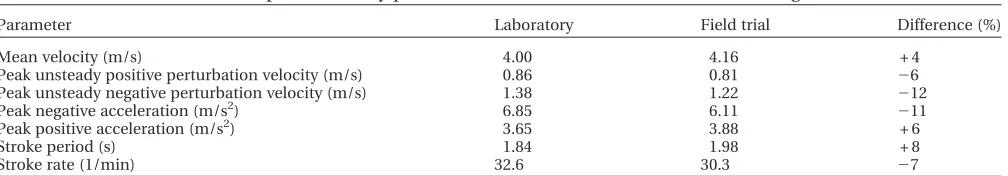
Several sections of trials data were identified as similar to the tank data in terms of velocity and acceleration. Key comparisons for one section of field data are shown in Table 2. Figure 7 shows the results for the gauges located 600 mm from the bow for these sections of the time-histories. The field-trial data have been processed in a number of ways here. In order to account for the minor varia-tion between the stroke periods in the field-trial time-histories, the data have been divided up into individual strokes, and the time value at each point normalized with respect to the appropriate stroke period. The field-trial hot-film data have also been offset for clarity and scaled to account for differ-ences in amplifier settings between field and tank

tests; scaling does not affect the validity of the comparison since the focus here is on the variation of signal with time rather than the absolute magni-tude of the signal. Finally the normalized accelera-tion values have been offset negatively by two units.

The periodicity of the hot-film and acceleration signals in the tank tests can be seen by superimpos-ing the four time-normalized cycles as shown in Fig. 8(a); the cycles were then averaged to produce Fig. 8(b). Similar plots for the field-trial data are shown in Figs 8(c) and 8(d). Here the greater varia-bility in the phases of the variations in the signal leads to averaged values which are rather reduced compared with the individual signals.

The velocity histories can be seen to be highly similar; however, the acceleration patterns exhibit greater differences, with the peak positive accelera-tion occurring at about t/T’0.45 in the tank tests and about t/T’0.55 in the field trials. It is pre-sumed that the discrepancies in the acceleration profile relate to differences in the ‘micro-phases’ of the drive phase, discussed by Kleshnev [11], corre-sponding to different parameters of the boat, rower, and oar kinematics.

The field-trial hot-film signals generally exhibit more variability than the data from the laboratory. This could be expected for three reasons: back-ground turbulence levels are very likely to be higher in the field trials; stroke-to-stroke variations are greater; finally the impact of athlete movement on heave and pitch will be variable in the field trials. Nonetheless it can be seen that many key features of the signal are comparable between laboratory and field data.

Both data sets show a large periodic peak sug-gesting onset of turbulent flow near peak

(a) Tank-test

(b) Field Trials

Velocity (m/s)

Hot Film output (V)

0.5 1.0 1.5 2.0 2.5 3.0 3.5 4.0 4.5 0.15 0.18 0.20 0.23 0.25 0.28 0.30 0.33 0.35 0.38 0.40 Outlier (HF Aft) HF Fwd (tripped) HF Fwd HF Aft Velocity (m/s)

Hot Film Output (V)

1.0 1.2 1.4 1.6 1.8 2.0 2.2 2.4 2.6 2.8 3.0 0.30 0.32 0.34 0.36 0.38 0.40 0.42 0.44

Fig. 5 Calibration curves for unsteady analysis

time (s)

Unsteady Hot Film Output (V)

Normalised Acceleration, Velocity

fast row comparison 1 run05

0.00 1.00 2.00 3.00 4.00 5.00 6.00 7.00 -2.00 -0.02 0.00 0.00 2.00 0.02 4.00 0.04 6.00 0.06 8.00 0.08 10.00

Unsteady HF Fwd Unsteady HF Aft

Normalised Acceleration Normalised Velocity

-0.04

deceleration (e.g.t/T’0.1–0.2). The relative magni-tude of the peaks varies rather more in the trials data than in the laboratory data. In the laboratory data, the high signal level is sustained from near the point of peak deceleration as the acceleration increases smoothly towards the maximum value, then the signal level drops once the acceleration peaks (e.g. t/T’0.4). In the field trial data, the sig-nal level drops around peak deceleration, rises again as the acceleration starts to increase (e.g.t/T’0.3), drops a second time as the acceleration momenta-rily levels out (e.g.t/T’0.4), then rises again as the acceleration increases once more (t/T’0.6), to cre-ate a distinct third peak.

Both data sets also show a second smaller set of periodic double peaks which correspond to a local minimum acceleration (e.g. t/T’0.9–1.0); these peaks are slightly more variable in the trials data, failing to appear in the second stroke shown.

The differences between the patterns of the hot-film signals are greater at the forward gauge. The time-normalized data averaged over the four cycles are shown in Fig. 9. Both signals show a small peak near the peak positive acceleration; the tank test data show a clear spike at peak deceleration t/

T’0.25, while the field trial data show a smaller

broader local maximum at this point. However, the field trial data show a large peak at aroundt/T’0.1, which is completely absent from the tank data. This corresponds to the point at which acceleration starts to reduce, and the maximum velocity. It is possible that the flow measurements at the forward gauge are more sensitive to the pitching dynamics of the hull than the flow further aft.

3.3 Further tank-test studies

A series of additional runs were carried out in the test tank in order to explore various aspects of the behaviour. In order to assess the relative importance of the mean velocity on the unsteady behaviour, the rowing pattern shown in Fig. 3 was repeated with the mean velocity reduced from 4.0 m/s to 3.0 m/s. Results for the aft gauge are shown in Fig. 10(a); it can be seen that the change in mean velocity (and hence mean Reynolds number) has remarkably little impact on the results. Results for the forward gauge showed a similar level of insensitivity to mean velo-city. This result suggests that Froude-scaled model tests utilizing correct acceleration profiles could cor-rectly identify the flow phenomena.

The impact of small changes in the acceleration pattern was also investigated. In this case, the results obtained using the pattern of Fig. 3 were compared with those obtained from a second pat-tern obtained from a ‘cruise’ (i.e. lower mean-velocity) part of the record. The stroke rate of the cruise pattern was increased by 50 per cent to be similar to that of the fast pattern for comparability. Results are shown in Fig. 10(b). It can be seen that the large peak at the catch is common to both sig-nals; however, the changes in the acceleration pat-tern during the drive phase of the stroke result in differences in the secondary peaks which are similar to those observed in the field-trial data.

A final set of tests was carried out to examine the impact of small waves on the phenomena. Figure 10(c) shows the impact of waves of ampli-tude 10 mm and frequency 1.25 Hz on the aft gauge. It can be seen that the results immediately become

Table 2 Comparison of key parameters for field-trial and tank-test data segments

Parameter Laboratory Field trial Difference (%)

Mean velocity (m/s) 4.00 4.16 + 4

Peak unsteady positive perturbation velocity (m/s) 0.86 0.81 26

Peak unsteady negative perturbation velocity (m/s) 1.38 1.22 212

Peak negative acceleration (m/s2) 6.85 6.11 211

Peak positive acceleration (m/s2_{) 3.65 3.88 + 6}

Stroke period (s) 1.84 1.98 + 8

Stroke rate (1/min) 32.6 30.3 27

more variable, resembling the field-trial results in their ‘noisy’ appearance.

4 RESISTANCE MEASUREMENTS

In order to place the results from the previous sec-tion into context, a series of resistance tests were

carried out. These were intended to indicate the scale of the likely benefits of delaying transition by a distance comparable to the 200 mm difference between the gauges in the hot-film measurements, both at steady speed and with a realistic periodic rowing motion.

The scull was set up in three configurations with regard to turbulence stimulation – with no stimulation,

with micro-studs applied at 400 mm from the bow, and at 600 mm from the bow. The micro-studs were 3.5 mm in diameter and 1.75 mm high, spaced 10 mm apart. In each case a calm-water resistance test was carried out over the speed range of interest, as well as a Prohaska test and a limited set of oscillatory tests.

A stud drag correction was applied using an esti-mate of the velocity distribution in a laminar bound-ary layer in conjunction with a bluff-body drag coefficient, as suggested by Molland et al. [12]. Naturally no attempt was made to correct for bound-ary layer effects, as identifying the magnitude of these effects was one of the goals of the tests. An analysis of uncertainty indicated that the 95 per cent confi-dence interval for uncertainty on the total resistance measurement was of the order of 0.5 per cent.

The resistance of the scull was decomposed in the conventional fashion

CT= RT

1=2rV2_S =CFð1 +kÞ+CW

Here CT is the total resistance coefficient,CFis the

flat-plate frictional coefficient, here based on the ITTC (International Towing Tank Conference) 1957 formulation, k is the form factor, CW is the wave

resistance coefficient, and S is the wetted surface area, here taken at the static waterline with the hull in level trim. It should be noted that in practice the

wetted area will vary dynamically during a stroke as the hull surges and pitches; it is also likely that the shape of the hull varies slightly both statically and dynamically from the unloaded condition owing to longitudinal bending.

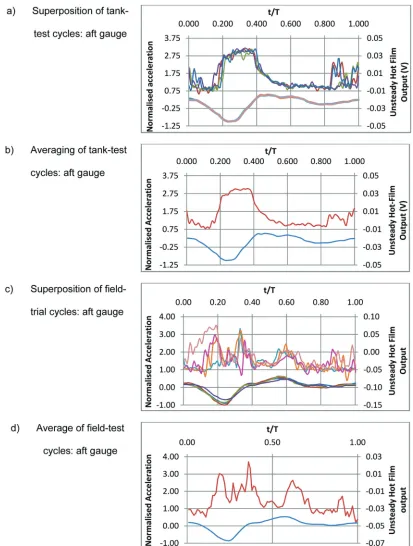
The form factor is obtained in the usual manner via a Prohaska test. The Prohaska plot for the tests with no turbulence stimulation is shown in Fig. 11(a); the test gives 1 +k= 1.012. These values are somewhat lower than those quoted by Scragg and Nelson [1], based on an unpublished study for the US Olympic Rowing Association. The Prohaska tests for the cases with studs at 600 mm and 400 mm yielded values of 1 +k= 1.013 and 1 +k=

1.022 respectively after stud drag correction.

Resistance tests were carried out at mean speeds of up to 4.0 m/s. These speeds yield a mean depth Froude number of around 0.9; hence any unsteady wave-making effects are of extremely long period (see Day et al. [13]). These effects are small for a slender hull such as this, but in order to ensure that they do not bias comparisons, care was taken to ensure that for each speed a similar section of the record was analysed. The total and viscous resis-tance coefficients are shown in Fig. 11(b). It can be seen that the wave-making resistance for this hull is significant at higher speeds, contributing over 15 per cent of the total steady-speed calm-water resistance at 4.0 m/s. It should be noted, however, that this

hull is relatively stable and beamy by the standards of single sculls; a more slender and more competi-tive hull would incur less wave-making resistance. It should also be noted that the mean depth Froude number in these tests is somewhat higher than

would be experienced in a rowing event, for which the water depth would typically be at least 3.0 m deep, yielding a depth Froude number of 0.74. This increase of depth Froude number is likely to increase the contribution of wave-making resistance in steady

speed compared with the value at the same speed in deeper water, but it seems unlikely that it would affect the viscous components of resistance.

The mean differences between the three different cases after correction for stud drag are summarized in Table 3. From these results it can be inferred that delaying transition by 200 mm can yield almost 0.5 per cent reduction in calm-water resistance; hence suggesting the possibility for improvement by subtle re-design of bow shape. The results for the studs at 400 mm are shown in Fig. 11(b).

In the final set of tests, the resistance was mea-sured in the rowing condition, using the trajectory of Fig. 3. Additionally, in order to examine the effect of gross simplification to the oscillatory profile, the sine wave best fitting the excursion profile in a least-squares sense was calculated and tested. This yielded an amplitude of 0.24 m, with the same period of 1.84 s.

Extreme care must be taken when analysing the resistance results with unsteady speed as the inertial loads are very large in comparison with the steady hydrodynamic loads, which in turn are large com-pared with the unsteady components. In the current study this was addressed by calculating a moving

average over a period equal to the oscillation period. The mean acceleration over this period is zero, and hence the mean inertial force is zero.

Unfortunately, owing to an error in programming the actuator during these tests, the load cell and towing point on the scull were seriously damaged (demonstrating the risks of working with such high-power devices), so only limited results were obtai-ned for a mean velocity of 4.0 m/s. These are summarized in Table 4.

It can be seen from these results that the effect of the realistic profile of unsteady speed increases the resistance by 2–3 per cent compared with the corre-sponding steady-speed case. These results fall within the range of data reported by Scragg and Nelson [1] who reported increase in resistance owing to surging of 2–5 per cent for the three one-third-scale hulls tested with turbulence stimulation.

The increase in resistance results from both unsteady wave-making and unsteady viscous effects. The high accelerations of the realistic rowing profile results in larger penalties in unsteady resis-tance than the sinusoidal oscillation, with an increase of 3.0 per cent for the rowing profile in the free-transition case (see Fig. 11(b)) compared with

1.8 per cent for the sinusoidal oscillation. It is inter-esting to note that the penalty for the rowing profile is greater where the laminar–turbulent transition is free, suggesting that part of this penalty relates to fluctuations in the location of transition owing to unsteady effects as discussed in the previous sec-tion. It is possible that the effect of reduced water depth in the current tests has subtly affected the variation in mean wave-making resistance; however, it is not necessarily obvious whether this change would exaggerate or reduce the impact of unsteadi-ness on wave-making resistance.

Finally, it should be stated that it seems quite likely that the penalties for unsteady speed will be higher for elite athletes, and for other types of row-ing shells which exhibit greater surgrow-ing accelera-tions than the single scull tested here.

5 DISCUSSION AND CONCLUSIONS

The study has examined the impact of unsteady effects on laminar–turbulent transition on a single scull in both laboratory and field-trial conditions. In both cases turbulence is shown to be strongly related to acceleration through the stroke cycle. Comparison of tank-test results with field-trial mea-surements show that the unsteady viscous flow phe-nomena identified in the real-world measurements are also present in the tank. Tests with similar oscil-latory patterns indicate that effects are relatively insensitive to mean velocity. It is shown that small changes in acceleration pattern can lead to signifi-cant changes in the time-history of transition; finally small waves can have a marked effect.

The practical relevance of the location of transition is shown by steady-speed resistance tests indicating that an aft movement of a forced transition point by

200 mm reduces resistance of a single scull by almost 0.5 per cent. A small number of tests with realistic unsteady velocity profile suggest that unsteady effects increased the resistance by about 3 per cent in cases in which the location of transition is not fixed, and 2.4 per cent where the location is fixed by studs. It can be suggested that these unsteady effects will be larger as peak accelerations increase both in other rowing events, and with elite athletes.

Future studies planned include an application of some of the current test methodologies to canoes and kayaks, and the investigation of the effects of unsteadiness on laminar–turbulent transition on the two-dimensional flow around a ‘friction-plane’ or plank representing a practical implementation of flat-plate flow.

ACKNOWLEDGEMENTS

This work was funded by the UK Engineering and Physical Sciences Research Council (EPSRC) under the ‘Achieving Gold’ program grants EP/F006284/1 and EP/F00625X/1. The authors are grateful to Dr Dominic Taunton of the Department of Ship Science at the University of Southampton for rowing in the field trials. They are indebted to Charles Keay and the technical staff of the Kelvin Hydrodynamics Lab for constructing the test rig, and to Ed Nixon for his help with the test programme.

ÓAuthors 2011

REFERENCES

1 Scragg, C. A. andNelson, B. D. The design of an eight-oared rowing shell. Marine Technol., 1993,

30(2), 84–99.

Table 3 Mean changes in resistance with location of turbulence stimulation

Case Compared with Mean difference in resistance (%)

Studs at 600 mm No studs 0.75

Studs at 400 mm Studs at 600 mm 0.43

Studs at 400 mm No studs 1.18

Table 4 Comparison of unsteady and steady resistance at mean velocity 4.0 m/s

Case Compared with

Difference (%)

Oscillation Stimulation Oscillation Stimulation

Sinusoidal No studs Steady No studs 1.8

Rowing profile No studs Steady No studs 3.0

Steady Studs at 400 mm Steady No studs 1.1

Sinusoidal Studs at 400 mm Steady Studs at 400 mm 1.9

2 Tuck, E. O. and Lazauskas, L. Low drag rowing shells. In Proceedings of the Third Conference on

Mathematics and computers in sport, Bond Univer-sity, Queensland, Australia, 1996, pp. 17–34.

3 Lazauskas, L. Rowing shell drag comparisons. Technical report L9701, Department of Mathe-matics, University of Adelaide, 1998, available from http://www.cyberiad.net/library/rowing/real/ real row.htm.

4 Formaggia, L., Miglio, E., Mola, A., and

Parolini, N. Fluid–structure interaction problems in free surface flows: application to boat dynamics.

Int. J. Numer. Methods Fluids, 2008,56, 965–978.

5 Formaggia, L., Miglio, E., Mola, A., and

Montano, A. A model for the dynamics of rowing boats. Int. J. Numer. Methods Fluids, 2009, 61, 119–143.

6 Berton, M., Alessandrini, B., Barre´, S., and

Kobus, J. M.Verification and validation in compu-tational fluid dynamics: application to both steady and unsteady rowing boats numerical simulations. In Proceedings of the 16th ISOPE Conference, Lis-bon, Portugal, 2007, vol. 3, pp. 2006–2011.

7 Wellicome, J. F. Report on resistance experiments carried out on three racing shells. National Physical Laboratory Ship T.M.184, 1967.

8 Doctors, L. J., Day, A. H.,andClelland, D. Resis-tance of a ship undergoing oscillatory motion. J. Ship Research, 2010,54(2), 120–132.

9 Kleshnev, V. Rowing Biomech. Newsl., 2002, 2, no. 6.

10 Binns, J. R., Albina, F. O.,andBurns, I. A.Looking for ‘laminars’: measuring intermittency on the

America’s Cup race course. Expl Thermal Fluid Sci., 2009,33, 865–874.

11 Kleshnev, V. Rowing Biomech. Newsl., 2002, 2, no. 11.

12 Molland, A. F., Wellicome, J. F.,andCouser, P. R.

Resistance experiments on a systematic series of high speed displacement catamaran forms: varia-tion of length-displacement ratio and breadth-draught ratio. Ship Science Report 71, Department of Ship Science, University of Southampton, 1994.

13 Day, A. H., Clelland, D.,andDoctors, L. J. Unstea-dy finite depth effects during resistance tests in a towing tank. J. Marine Sci. Technol., 2009, 14(3), 387–398.

APPENDIX

Notation

CF flat-plate frictional resistance coefficient

CT total resistance coefficient

CW wave resistance coefficient

k form factor

RT total resistance

S wetted area

t instantaneous time

T oscillation period

V velocity