The impact of immigrant dynasties on wage inequality

City, University of London Institutional Repository

Citation

: Ben-Gad, M. (2006). The impact of immigrant dynasties on wage inequality.

10.1016/S0147-9121(05)24003-7

This is the unspecified version of the paper.

This version of the publication may differ from the final published

version.

Permanent repository link:

Link to published version

: http://dx.doi.org/10.1016/S0147-9121(05)24003-7

Copyright and reuse:

City Research Online aims to make research

outputs of City, University of London available to a wider audience.

Copyright and Moral Rights remain with the author(s) and/or copyright

holders. URLs from City Research Online may be freely distributed and

linked to.

City Research Online: http://openaccess.city.ac.uk/ publications@city.ac.uk

The Impact of Immigrant Dynasties on Wage Inequality

Michael Ben-Gad

University of Haifa

June

2005

Abstract

I construct a set of dynamic macroeconomic models to analyze the effect of unskilled immi-gration on wage inequality. The immigrants or their descendants do not remain unskilled–over time they may approach or exceed the general level of educational attainment. In the baseline model, the economy’s capital supply is determined endogenously by the savings behavior of infinite-lived dynasties, and I also consider models in which the supply of capital is perfectly elastic, or exogenously determined. I derive a simple formula that determines the time dis-counted value of the skill premium enjoyed by college-educated workers following a change in the rate of immigration for unskilled workers, or a change in the degree or rate at which unskilled immigrants become skilled. I compare the calculations of the skill premiums to data from the U.S. Current Population Survey to determine the long-run effect of different immigrant groups on wage inequality in the United States.

JEL Classification Numbers: J61, O41.

Key Words: Immigration, Educational Attainment, Wage Inequality.

1

Introduction

In this paper I construct a set of macroeconomic models to analyze how increases in the number

of unskilled immigrants may affect wage inequality over time. In these models, a change in

the number of such immigrants does not necessarily alter the composition of the workforce

permanently. Rather than remaining unskilled forever, a portion of the additional immigrants,

or their descendants, join the ranks of skilled workers. Indeed, as is the case for some immigrant

groups in the United States, the native-born children or grandchildren of immigrants with low

levels of education may not merely assimilate by matching the general level of educational

attainment, but exceed it.

For the baseline model, I adopt the Weil (1989) overlapping dynasties optimal growth

frame-work. Changes in immigration policy not only affect wages directly by altering the size and

composition of the labor force, but also alter the rate of return to capital, inducing changes in

savings behavior that gradually affect the size of the capital stock. These changes to the size of

the capital stock indirectly affect wages as well. I derive a simple reduced form that encapsulates

all these different effects on one measure of wage inequality–the ratio between the discounted

values of skilled and unskilled wages.

The effect of a change in immigration policy on wages is neither constant nor immediate. A

change in immigration policy generates changes in the size and composition of the population

that accumulate over time. The effect of these changes on factor returns may or may not be

permanent, depending on whether the labor supplied by the immigrants or their descendents

perfectly substitutes for the pre-existing labor supply. Therefore by examining the ratio between

the discounted value of the two different wages, I can determine to what degree, in the long run,

high educational attainment by the descendants of unskilled immigrants either ameliorates or

reverses their short-run impact on wage inequality.

In my baseline model, capital is endogenously determined but adjusts slowly. Borjas (1999)

analyzes the impact of immigration in static models under two alternative assumptions–capital

supply is either completely elastic, orfixed. To better understand the sensitivity of my measure

of wage inequality to different assumptions about the supply of capital, I compare the behavior

of my model to one in which the stock of capital adjusts immediately to policy changes, but

where the rate of return is exogenously determined. In addition, I also consider the case where

the size of the capital stock grows at a fixed exogenous rate.

In Section 2, I briefly review recent U.S. immigration policy. I present data from the U.S.

Census Current Population Survey that demonstrates the vast differences in educational

at-tainment among different immigrant groups–differences that span at least two generations.

These data also highlight the higher degree of intergenerational mobility between the immigrant

I present in Section 3 the dynamic optimal growth model with overlapping dynasties,

devel-oped by Weil (1989). Ben-Gad (2004) used the model to examine the behavior of an economy

that is absorbing immigrant dynasties over time. In this paper, I distinguish between two types

of households: households with skilled workers (college-educated adults), with unskilled workers

(adults without college degrees).

Section 4 describes the dynamic system and the general perturbations method I use to

simulate its behavior. I also derive the formula used to calculate the discounted skill premium

(the percentage gap between the present value of wages for college and non-college educated

workers) in the baseline model. I also present the explicit reduced form for the special case

where the elasticities of substitution between the factors of production are all identical.

Section 5 briefly describes two alternative assumptions about the elasticity of the capital

supply. I demonstrate that for the special case in which all the elasticities of substitution

between the inputs are identical, the ratio between the two wages at any moment in time is

identical, regardless of what mechanism governs the dynamic behavior of the capital stock.

Nonetheless, even in this case, the discounted premium to education is sensitive to the model

we choose.

In Section 6, I present my procedure for modelling the effect of immigration policy on the

composition of the labor force over time. There is first, a direct effect as the ratio of skilled to

unskilled workers among the extra new arrivals seldom matches the veteran population. There

is a second effect because I permit the descendants of these immigrants to switch between the

two categories during the periods after they arrive. One serious limitation to this approach is

that membership in either category is determined exogenously–I am modeling the impact of

observed changes in educational attainment but make no attempt to explain them.

Section 7 explains the choice of parameters I use to calibrate the model. In Section 8, I

consider the impact of a twenty-year surge in the immigration of unskilled workers on wages

and wage inequality, within the context of three different assumptions for the elasticity of capital

supply, and three different specifications of the production function. I consider three different

scenarios. First, what if the immigrants and their descendants remain permanently unskilled?

No one ever attends college, and their arrival permanently lowers the share of unskilled workers

within the economy. This scenario is a crude approximation of perhaps the most pessimistic

outcome for immigration: the creation of a permanent unskilled under class. In the second

scenario, the immigrants are initially unskilled, but over time, they or their descendents

grad-ually attain the levels of college education prevalent in the general population. This process of

immigrant ‘assimilation’ ultimately restores the distribution of college-educated and non-college

educated people in the workforce to its initial level. In the third scenario all the immigrants

or their descendents eventually attend college. This last case is perhaps the least likely, yet

identically sized influx of college-educated immigrants.

Finally, in Section 9, I consider more realistic examples, where not all immigrants are skilled

or unskilled and neither are all their descendants. I relate the results for the discounted skill

premium to the data on college attainment for the different immigrant groups in the Current

Population Survey.

In this paper I do not presume to explain the decisions made by households to immigrate.

Because legal migration from the developing world to the developed world is regulated by the

rationing of visas, and illegal migration by the resources invested in interdiction, or the harshness

of penalties imposed on those violating immigration laws, I believe it is possible to treat modest

changes in rates of immigration for unskilled workers as exogenous policy decisions.1 More

importantly, this paper ignores the decisions made by immigrants or their descendants to acquire

education. Instead, I focus on the long-run implications of differential educational attainment

among immigrants and their descendents for wage inequality.

2

U.S. Immigration Policy and Educational Attainment Among

Immigrant Groups

2.1

The Rate of Net International Migration

The share of foreign-born within the population of the United States declined steadily between

1910 to 1970, from 14.7% to 4.7%. Since then it has climbed swiftly, reaching 11.7% by the end

of 2003. What has generated such a dramatic rise in just over three decades?

The official rate of immigration presented in Figure 1, Panel a), features the data tabulated

by the U.S. Bureau of Citizenship and Immigration Services. These numbers show immigration

rising steadily from a rate of 1.5 per thousand in 1960 to 2.6 per thousand in 1988, then rising

much more steeply, reaching 7.1 per thousand in 1991, and then declining to 2.3 per thousand

in 1999.

The rate at which people arrived in the United States did indeed rise between 1960 and 1991,

but not by nearly so much, nor was the rate nearly so volatile. The official rate of immigration in

Panel a) of Figure 1 does not show the date at which foreigners arrive in the United States or join

its workforce, but merely captures the number who attain the official status of immigrant. Hence

there was no massive influx of immigrants in 1991, but rather a large number of people, many

living and working illegally in the United States for a decade or more, who took advantage of

the amnesty provisions in the Immigration Reform and Control Act of 1986 (IRCA), to register

as legal immigrants.

1

See Galor (1986), Djajic (1989), Borjas (1994), and Zak et. al. (2002) for models with endogenously

Figure 1: Annual rates per thousand, of legal immigration and components of population growth in the United States, 1960 to 1999. Natural population growth is number of births, less deaths. Net international migration (NIM) from 1960 to 1984 includes migration by U.S. civillians, but excludes military personnel, NIM from 1985 to 1994 excludes both U.S. civillians and military personnel, and 1995 to 1999 NIM excludes both U.S. civillians and military personnel. The dashed gray lines correspond to decade averages for NIM.Sources: U.S. Census Bureau, Population Division and Housing and Household

Economic Statistics Division and U.S. Census Bureau, Statistical Abstract of the United States, various

years.

1981

1960 1963 1966 1969 1972 1975 1978 1981 1984 1987 1990 1993 1996 1999 1

2 3 4 5 6 7 8 9 10 11 12 13 14

bLComponents of Population Change in the United States 1981-1999

Natural Pop. Growth

Net International Migration 1981

1960 1963 1966 1969 1972 1975 1978 1981 1984 1987 1990 1993 1996 1999 1

2 3 4 5 6 7 8 9 10 11 12 13 14

Net international migration (NIM) in Figure 1 Panel b), measures the physical movement

of people between the United States and the rest of the world. The rise in the NIM was far less

dramatic than either the changes in the official rate of immigration or the steep decline in the

rate of natural population growth in Panel b) of Figure 1.2 Between 1960 and 1999 the birth

rate in the United States dropped from 23.8 to 14.4 per thousand, causing the steep decline in

the rate of natural population growth. The sharp decline in the birth rate combined with the

gradual increase in net migration between 1970 and 2000 to generate the large increase in the

share of the foreign born within the U.S. population over the same period.

2.2

U.S. Immigration Policy

Since passage of the Immigrant and Nationality Act of 1965, most legal immigrants have

ar-rived in the United States through some form of family sponsorship. Immediate relatives of

United States citizens may enter without limit; during the 1990’s about a quarter of a million

arrived each year. Other relatives of U.S. citizens are admitted as family-sponsored preference

immigrants–the Immigration Act of 1990 set the limit for all family sponsored immigrants as

either 226,000, or 480,000 minus the number of people admitted under the category of

imme-diate relatives during the previous year, whichever is larger. The United States also allocates

140,000 employment-based preference visas for workers with special skills or training (as well

as investors), and an additional 55,000 visas are allocated by lottery under the diversity

pro-gram. Finally, the United States admits refugees and asylum seekers (refugees are admitted

from abroad on the basis of a yearly quota set annually by the president). After a year, refugees

and asylees are eligible for permanent residence–between 1991 and 2000, just over one million

gained admission.

In addition to immigration visas, in 1992 the United States began granting 65,000 H-1B

visas to temporary workers with special skills–nearly all recipients have college or advanced

degrees.3 To ameliorate a perceived shortage of qualified workers in the information technology

sector, Congress passed the American Competitiveness in the Workforce Act of 1998, temporarily

increasing the number of H-1B visas to 115,000 per year in 1999 and 2000, and 107,500 in 2001.

The American Competitiveness in the Twenty-First Century Act of 2000 (AC21) added an extra

347,500 visas by raising the cap to 195,000 for each of the years 2001, 2002, and 2003, for a total

of 585,000 H-1B visas over three years. The cap for 2004 and beyond is once again 65,000.

2

Data for the rate of net international migration are available for calender years up until 1999, and for years

2001 and beyond. Data for 2000 are available for only part of the year. Therefore I compare the decades 1960-1969,

1970-1979, 1980-1989, 1990-1999.

3_{H-1B visas are granted for a maximum of two consecutive three-year stays. However, workers are no longer}

required to demonstrate an intention to return to their home countries and most recipients are soon eligible to

apply for permanent residency. In the past at least half of those admitted under the program changed status and

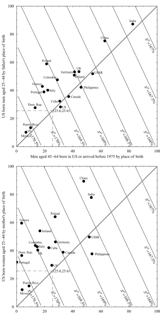
Figure 2: Percentage of the U.S. population with four-year college degrees by age, sex, birthplace, and parent’s birthplace. Data for the USSR includes all respndents from any of the former republics in the sample, the data for the UK includes respondents from Northern Ireland, and data for Portugal includes respondents from the Azores. Pooled data for 2001, 2002, and 2003 from the U.S. Census, Current Population Survey. Source: Miriam King, Steven Ruggles, and Matthew Sobek. Integrated Public Use Microdata Series, Current Population Survey: Preliminary Version 0.1. Minneapolis: Minnesota

0 20 40 60 80 100

Women aged 45-64 born in US or arrived before 1975 by place of birth

0 20 40 60 80 100 S Un ro bn e mo wd eg a5 2 -44y br eht o m' s ec al pf oh tri b US Mexico Puerto Rico Italy Canada Germany Philippines Cuba UK Ireland China Poland Portugal USSR India Dom. Rep. Greece Colombia

y=31.34+0.59x

R2_=.30

0 20 40 60 80 100

Men aged 45-64 born in US or arrived before 1975 by place of birth

0 20 40 60 80 100 S Un ro bn e md eg a5 2 -44y br eht af' s ec al pf oh tri b US Mexico Puerto Rico Italy Canada Germany Philippines Cuba UK Ireland China Poland Portugal USSR India Dom. Rep. Greece Colombia

y=16.07+0.82x

Finally, the gross inflow of illegal immigrants is about 350,000 per year.4 The net increment

to the population from this source is smaller–eighty percent of those who leave the United

States are foreign born, and a substantial fraction of these are illegal aliens returning home. In

the year 2000 there were approximately seven million people living in the United States illegally,

of whom 1.5 million arrived between 1991 and 2000–a net inflow of 150,000 per year.5

2.3

College Attainment and Immigrant Groups

Clearly, any government considering a serious change in its immigration policy should be

con-cerned not only with the skills immigrants bring to their new country, but also with the levels of

education attained by their children–the members of the second generation. In the two graphs

in Figure 2, I pool data from the Current Population Survey of the U.S. Census for the years

2001, 2002, and 2003. The horizontal axes correspond to the share of people aged 45-64 with

four-year Bachelor’s degrees by place of birth. I sample only those immigrants who arrived

prior to 1975. So as to focus on people who have immigrated to the United States near the

beginning of their working lives, and at about the time they are establishing a household. By

restricting the sample I exclude older people whose immigration was perhaps sponsored by their

adult children–themselves immigrants to the United States.

Examining immigrants by country of origin reveals an enormous degree of heterogeneity in

the shares of people with college degrees. By this measure, male immigrants from India are the

best educated–nearly 83% have college degrees, followed by male immigrants from China with

63%. By contrast, the average share of college educated U.S. born males within the same age

group is only 31%.

Among all the males in this sample, the least educated are Mexican immigrants, of whom

just under 7% have completed college, followed by Puerto Ricans (I treat respondents who report

Puerto Rico as their birthplace as immigrants rather than natives even though they are U.S.

citizens by birth). Although formal education does not completely encompass all labor market

skills or perfectly predict labor market outcomes, it is not hard to imagine the direct impact of

these immigrants from Mexico or Puerto Rico on the wages of unskilled workers in the United

States. Indeed, Borjas (2003) estimates the overall wage elasticity within skill groups to be -0.4

(there are four levels of educational attainment in his model, and he also controls for labor force

experience).

By contrast the arrival of highly educated immigrants from India or China is likely to depress

the wages of skilled workers. Abstracting from the overall level of wages, further immigration

4

U.S. Department of Homeland Security, Office of Immigration Statisitics, 2002 Yearbook of Immigration Statistics.

5_{U.S. Immigration and Naturalization Service, Office of Policy and Planning, Estimates of the Unauthorized}

from India or China is likely to lower the wage premium enjoyed by male college graduates,

whereas immigration from Mexico and Puerto Rico is likely to enhance it. Furthermore, the

impact of each particular group of immigrants on the composition of the labor force and wage

inequality is likely to last long after the immigrants themselves retire.

To understand what this means, consider the vertical axes of the graphs in Figure 2. These

measure the rate of college completion among U.S. born individuals aged 25-44, according to

the birthplace of their fathers (for men) or mothers (for women). These are members of a

second generation, counterparts to the immigrant generation whose rates of college education

are measured on the horizontal axis.

Notice that in the upper panel of Figure 2, the points representing Mexico, Puerto Rico and

India are above, but fairly close to the solid grey 45◦ line through the origin, and the point

representing China is not too far from it either. If we treat the younger people in our sample,

represented on the vertical axes as surrogates for the children of the immigrant cohort on the

horizontal axes, we can conclude that the impact of each immigrant group on the share of college

educated within the population is fairly constant over the course of at least two generations.

This does not mean that their quantitative impact on wages is constant–the overall level of

wages, and under some circumstances the ratio between wages for skilled and unskilled workers,

is very dependent on the rate of adjustment of the capital stock to any surge in immigration.

Nonetheless, qualitatively, we can confidently predict the impact on wage inequality generated

by each of these four immigrant groups across at least two generations and probably more.6

This confidence quickly dissipates when we consider some of the other groups represented in

Figure 2, or worse still, when we attempt to compare between them. Among male immigrants

from Poland in our sample, only 21% have college degrees–well below the average for the

pop-ulation as a whole. Yet the levels of college graduation among young American-born sons of

Polish-born fathers are immediately below the high levels attained by their Indian and Chinese

counterparts–59% in the sample completed college. How do we compare the impact of male

immigrants from places like Poland, with their high levels of intergenerational upward mobility,

with the impact of better educated immigrants from Colombia, Cuba, Germany, Ireland, Italy

or the United Kingdom? How much does it matter that the children of these more-educated

im-migrants seem to experience relatively little upward mobility, and graduate from college at lower

rates than men whose fathers are from Poland? Indeed, what about immigrants from Canada,

the Philippines or the former USSR? There we see a slight drop across the two generations in

the share who report completing college.

Chiswick (1978) found that controlling for various factors, including age, and schooling,

immigrants to the United States earn more than their native counterparts provided they have

6

Considering recent studies on intergenerational mobility (see the survey by Solon (1999)) or the model of

worked in the U.S. for a long enough period of time. If we interpret this finding as a measure

of motivation, it would seem that some of this motivation spills over to the next generation or

is expressed in a greater effort by immigrant parents to provide a college education for their

children. Among males, the Polish immigrant group presents the most obvious example of this

phenomenon. However, nearly all the points in Figure 2 cluster along a regression line (R2 _=.68)

above the 45◦ line.7

The intergenerational outcomes for the women among these same immigrant groups in the

lower panel of Figure 2 are far less predictable. Consider female immigrants from Greece. In

terms of college completion, they are as a group the second least educated people in our sample.

Less than four percent of this group have college degrees, while among the American-born women

between the ages of 45 and 64 in our sample, the rate of college completion is 25%. Indeed,

only women born in Portugal have lower rates of college completion (.5%). Yet the point in

the lower panel of Figure 2 corresponding to Greece is well above the 45◦ line. This is because

just under 60% of second generation American born women aged 25 to 44 who report having

Greek-born mothers completed college, twice the rate of daughters of American-born women

in the same age group, and behind only women with mothers from China, India, and Poland.

What does the arrival of immigrants like these women from Greece mean for wage inequality in

the U.S. over time? Which dominates, the low levels of education in thefirst, or the high levels

of education in the second generation and perhaps beyond?

3

Immigration in a model with endogenous capital

accumula-tion

Suppose there are only two types of workers in the economy, either skilled or unskilled, and each

supplies a distinct labor input. These workers are members of infinite-lived households that

grow in size at a constant rate, and the number of these households is constantly augmented by

immigration.

To model an economy with both natural population growth and immigration, we treat each

resident as a member of an infinite-lived immigrant dynasty. In the absence of uncertainty, the

behavior of each new immigrant of typei,and all of his or her descendants, can be characterized

as the maximization of the dynasties’ infinite horizon discounted utility function beginning at

times:

max

ci

Z _∞

s

e(ρ−n)(s−t)lnci(s, t)dt, i∈{U, S}, (1)

subject to a time tbudget constraint:

·

ki(s, t) =wi(t)li+ (r(t)−n)ki(s, t)−ci(s, t), ∀s, t, i∈{U, S}, (2)

whereci(s, t),and ki(s, t) represent the timetconsumption and holdings of capital of the

mem-bers of a typeidynasty with arrival date s;wi(t) andr(t) represent their timetwages and the

rate of return of capital;ρis the subjective discount rate; andnis the rate of natural population

increase–the rate of growth of the dynasties themselves.

The consumption rule for dynasty sat timetis:

ci(s, t) = (ρ−n) [ωi(t) +ki(s, t)], ∀s, t, i∈{U, S}, (3)

whereωi(t) =

R_∞

t e−

Ru

t r(v)dvw_i(u)l_idu is the present discounted value of all future income from

labor of typeifrom timetforward. Immigrant households of typeienter the economy at timet

at a rate of mi(t), and we assume that all immigrants arrive in their new homeland. Aggregate

consumption and capital evolve according to:

˙

Ci(t) = (ρ−n) [r(t) (Ωi(t) +Ki(t))−Ci(t) +Pi(t)mi(t)ωi(t) ], i∈{U, S}, (4)

·

Ki(t) =wi(t)Li(t) +r(t)Ki(t)−Ci(t) (5)

whereCi(t), Ki(t), andΩi(t)are, respectively, the timetconsumption, physical capital holdings,

and the present value of future earnings aggregated over all the households with skill-level i;

Mi(s) is the number of households with skill-level i, that have accumulated by time s; and

Pi(s) = en(t−b)Mi(s) represents the overall size of each portion of the population.8 The total

labor input supplied by a household of type i_{∈ {}U, S_} at time t is li, and the total supply of

each type isLi(t) =Pi(t)li , i∈{U, S}.

The production function F :_R3 _{→ R} has constant returns to scale in both types of labor

and aggregate capital. Factors receive their marginal products:

r(t) =FK(kU(t) +η(t)kS(t), lU, η(t)lS)−δ, (6)

wi(t) =FHi(kU(t) +η(t)kS(t), lU, η(t)lS), (7)

where η(t) =PS(t)/PU(t) is the ratio of households with skilled workers to unskilled workers

in the economy at time t, and δ is the rate of depreciation for physical capital.

The behavior of the economy is determined by four laws of motion for per-capita consumption

ci(t) = C_Pi_i((_tt)₎ and capitalki(t) = K_Pii₍(_tt₎):

·

ci(t) = (r(t)−ρ)ci(t)−(ρ−n)ki(t)mi(t)κi(t) i∈{U, S}, (8)

8_{Define t= bas a date in the arbitrarily distant past b < 0, when the economy was founded by an initial}

cohort of sizeMU(b)+MS(b). ThenCi(t), Ki(t), andΩi(t)are the consumption, capital and the future earnings for the initial type i population at time b, and all the additional cohorts accumulated at rate mi(s) since b,

all growing at the rate ofn. Hence Ci(t)=en(t−b)R_btMi(s)mi(s)ci(s, t)ds+en(t−b)Mi(b)ci(b, t), Ki(t) =en(t−b)

Rt

bMi(s)mi(s)ki(s, t)ds+e n(t−b)_M

i(b)ki(b, t), Ωi(t)=en(t−b)³R_btMi(s)mi(s)ds+Mi(b)

´

ωi(t), andMi(s) =

·

ki(t) =wi(t)li+ (r(t)−n−mi(t)κi(t))ki(t)−ci(t) i∈{U, S}, (9)

where κi(t) = (ki(t)−ki(t, t))/ki(t) is the fractional difference between per-capita capital

holdings and the capital immigrants bring with them.

In our simulations we analyze the model using a family of production functions whose most

general expression is the nested constant elasticity of substitution (nested CES) aggregate

pro-duction function with constant returns to scale developed by Sato (1967):

F(K(t), LU(t), LS(t)) =

h

(1₋α)LU(t)ϑ+α(βK(t)υ+ (1−β)LS(t)υ)

ϑ υ

i1

ϑ

, (10)

where K(t) =KU(t) +KS(t) is the total stock of capital.9

4

The Dynamic System, and the Discounted Skill Premium

The sets of equations (8) and (9) for each skill-type are very similar, as the savings and

consump-tion decisions of each type of household in the economy are not very different from each other.

Finding a sufficiently precise approximation of the saddle path that corresponds to this dynamic

system is very difficult because the condition number of the Jacobian matrix of the linearized

system is very high. To overcome this problem, we define the variables aU(t) = ln ˜cU(t) and

χ(t) = ωS(t)

ωU(t), which equals

cS(t)−(ρ−n)kS(t)

cU(t)−(ρ−n)kU(t), and replace the two laws of motion for consumption

(8) with:

˙

aU(t) =r(t)−ρ−(ρ−n)e−aU(t)kU(t)mU(t)κU(t) (11)

˙

χ(t) = (ρ₋n) χ(t)wU(t)−wS(t)

eaU(t)_−(ρ−n)k

U(t)

(12)

·

kU(t) =wU(t) + (r(t)−n−mU(t)κU(t))kU(t)−eaU(t) (13)

·

kS(t) =wS(t) + (r(t)−ρ−mS(t)κS(t))kS(t) +

³

(ρ₋n)kU(t)−eaU(t)

´

χ(t) (14)

Redefining the variables of the system has an additional benefit. The variable χ(t) directly

expresses the ratio between the discounted values of all the future skilled and unskilled wages.

In steady state, rates of immigration for skilled and unskilled must be equal–we employ

perturbation methods (see Judd (1998)) to study the dynamic behavior of the model following

temporary changes in the flow of skilled or unskilled immigrants.10 Define m as the initial

9

Also known as the two stage CES production function. Thefirst stage combines skilled labor and raw capital

to develop and maintain production capital: K∗= (λKν+ (1−λ) (HS)ν)

1

ν_{. K}∗_{is used by unskilled labor in}

the second stage to manufacturefinal goods: Y =hµ(HU)ϑ+ (1−µ) (K∗)ϑ

i1 ϑ

.See Goldin and Katz (1998). 1 0_{The general theory of perturbations wasfirst developed by Euler, Laplace, and most importantly Lagrange}

in the late 18th century to study celestial mechanics. The movement of a planet around the sun was ‘perturbed’

from its eliptical orbit by the gravitational pull of other planets which varied over time (Ekeland (1988)). Judd

(1982), (1985) introduced perturbations to economics to studyfiscal policy where the perturbations are changes

steady state rate of immigration, and replace mi(t) in (11)-(14) with m+ πi(t), where πi(t)

is a bounded dynamic perturbation to the rate of migration by type-iworkers, and is a small

positive number that regulates its magnitude. Similarly we define η as the steady-state ratio

of skilled to unskilled workers and replace the the terms σ(t) with η+ ξ(t), where ξ(t) is a

bounded dynamic perturbation to the skill ratio.

Definingπ(t) =_{πS(t), πU(t)}∞_t=0, consumption and capital for each skill-type are all

func-tions of π,ξ and .11 We differentiate (8), (9) with respect to at the point = 0:       ∂ ∂ ·

aU(t, , π, ξ)

∂

∂ χ(t, , π, ξ)˙ ∂

∂ ·

kU(t, , π, ξ)

∂ ∂ ·

kS(t, , π, ξ)

     =J

     ∂

∂ aU(t, , π, ξ)

∂

∂ χ(t, , π, ξ) ∂

∂ kU(t, , π, ξ)

∂

∂ kU(t, , π, ξ)

    −     

(ρ₋n)e−aU_k

UκUπU(t)

0 kUκUπU(t)

kSκSπS(t)

    −      ΩK

(ρ−n)(χlUΩU−lSΩS)

eaU₋(ρ−n)kU

kUΩK+lUΩU

kSΩK+lSΩS

    ξ(t),

(15)

where Jis a 4_×4 Jacobian matrix; aU, χ, kU, and kS are the initial steady state values of log

consumption, the ratio between the present values of skilled and unskilled wages, and capital;

and ΩK=lS ∂

2_F

∂LS∂K +kS

∂2_F

∂K∂K,ΩU =lS ∂2_F

∂LS∂LU +kS

∂2_F

∂K∂LU,ΩS =lS

∂2_F

∂LS∂LS +kS

∂2_F

∂K∂LS.

To better understand how immigration affects the behavior of the model, I divide the shocks

in (15) between two separate vectors that operate autonomously. Thefirst contains the termsκU

andκS, and if positive [negative] reflects the effects of capital dilution [enhancement] generated

by the arrival of capital-poor [rich] immigrants, as described by Borjas (1995) in his static

model and Ben-Gad (2004) in a dynamic setting. The terms ΩK, ΩU, and ΩS in the second

shock vector, capture those changes in the returns to capital, unskilled wages, and skilled wages

respectively, that result from the change in the composition of the labor force, i.e. ξ(t).

The portion of a policy change that operates through the channel represented by the first

vector are completely transitory if the shocks have bounded support. Even permanent changes

in the rate of immigration produce few changes in factor returns, or in the welfare of the

native population. By contrast, the second vector can generate permanent changes in the

economy even if the policy changes it represents are transitory. Small differences in the rate of

immigration between the two types of immigrants accumulate over time, and permanently affect

the composition of the labor force. Only if the value of all the perturbations operating through

the second vector is zero in the limit–as will be the case if immigrant dynasties gradually

assimilate until they replicate the overall skill distribution–do all the variables in the economy

return to their original steady-state values.

1 1_{To guarantee convergence to an interior balanced growth path we also impose the restriction onπ}

S(t)and

πU(t)that they must satisfy

¯ ¯ ¯lim

T→∞

RT

0 (πS(t)−πU(t))dt

We solve (15) using Laplace Transforms:      Lv £_∂

∂ aU(t, , π, ξ)

¤

Lv

£_∂

∂ χ(t, , π, ξ)

¤

Lv

£_∂

∂ kU(t, , π, ξ)

¤

Lv

£_∂

∂ kU(t, , π, ξ)

¤      (16)

= (vI₋J)−1

          ∂

∂ aU(0, , π, ξ)

∂

∂ χ(0, , π, ξ)

0 0     −     

(ρ₋n)e−aU_k

UκULv[πU]

0 κUkULv[πU]

κSkSLv[πS]

    −      ΩK

(ρ−n)(χlUΩU−lSΩS)

eaU₋(ρ−n)kU

kUΩK +lUΩU

kSΩK+lSΩS

    Lv[ξ]

    

where _∂∂aU(0, , π, ξ) and _∂∂χ(0, , π, ξ) are the initial changes in the values of the two control

variables12. The matrix Jhas four eigenvalues, two negative and two positive. Define the two

positive eigenvalues as µ₁ and µ₂. Each element of the left-hand vector must be bounded for

any positive value v, including the eigenvaluesµ₁ and µ₂, and yet the determinants _|µ_hI₋J_|,

h _∈{1,2_} are zero by definition. The only way for (16) to be bounded when v=µ_h, h_∈{1,2_}

is for the numerator, the adjoint of µ_hI₋J, h _∈{1,2_} multiplied by the term in parentheses,

to be equal to zero:

adj [µ_hI₋J]

          ∂

∂ aU(0, , π, ξ)

∂

∂ χ(0, , π, ξ)

0 0     −     

(ρ₋n)e−aU_k

UκULµh[πU]

0 κUkULµh[πU]

κSkSLµh[πS]

    −      ΩK

ρ−n(χlUΩU−lSΩS)

eaU₋(ρ−n)kU

kUΩK+lUΩU

kSΩK+lSΩS

    Lµh[ξ]

    

= 0, h_∈{1,2_} (17)

both of which can then be solved for the values of _∂∂aU(0, , π, ξ)and _∂∂χ(0, , π, ξ).

Whereas the evolution of χ(t), the ratio between the present discounted value of skilled and

unskilled wages, is not of particular interest, (19)–the change in its value at timet= 0–gives

us all the relevant information for determining how a change in immigration affects discounted

wage inequality over time–without explicitly calculating the impulse responses for wages or

the rate of return to capital following a policy announcement. The discounted skill (or college)

premium SP is the percentage difference between the present discounted value of skilled and

unskilled wages:

SP = µ

χ+ ∂

∂ χ(0, , π, ξ)−1 ¶

×100 (18)

whereχ is once again the initial steady-state value ofχ(t).

The first element in the second row of matrix J is zero. The third and fourth are zero as

well, if the elasticities of substitution between the various inputs in the production function are

equal–ifυ=ϑin (10), only the diagonal elementJ22of the second row of matrixJis non-zero,

which is one of the two positive eigenvalues. Hence, the value of _∂∂χ(0, , π, ξ) is the second

1 2

The Laplace transform of a functionf(t)and a positive numbervisLv[f] =

R∞

0 f(t)e

−vt

element in the third vector in (17), where the eigenvalue is J22=ρ₋n:

∂

∂ χ(0, , π, ξ) =−

(ρ₋n) (χlUΩU−lSΩS)

eaU _{−(ρ−n)kU}

Z _∞

0

e−(ρ−n)tξ(t)dt (19)

Result 1 If the elasticities of substitution between all the inputs are equal, the discounted skill

premium is not a function of capital dilution κU and κS.

Result 1 tells us that even though the rate of return to capital is affected by changes in

immigration policy, for the special case of Cobb-Douglas or CES production, capital dilution

itself has no effect on the discounted wage gap. A surge in immigration of typeicertainly lowers

the wages of all the workers of type i in the economy as long as the values of κU and κS are

not negative. The wages of typej ₆=imay either rise or fall depending on whether the relative

scarcity of this type of labor has a stronger effect than the decline in per-capita capital. Either

way, as long as the elasticity of substitution between the inputs is constant, we can separate

the analysis of the discounted skill premium from the effects on the economy generated by the

dilution of the capital stock.

If F is CRS and all the inputs are complementary in production,Fij >0 for alli6=j then

ΩU > 0 and ΩS < 0. Furthermore _eaU₋(ρ(−ρ−n)n)kU = 1/ωU(t), the inverse value of the per-capita

present value of unskilled wages.

Result 2 If the elasticities of substitution between all the inputs are equal, the production

func-tion is CRS and all the inputs are complementary in producfunc-tion, the college premium increases

[decreases] if the present value of the shock ξ(t), discounted byρ₋n, is negative [positive].

From Result 2 we know how skilled and unskilled workers fare relative to each other, but

we do not know what happens to the overall level of wages in the economy. To calculate the

dynamic behavior of the wage levels we need to know the evolution of capital over time. We

apply the inverse Laplace transforms to (16):      ∂

∂ aU(t, , π, ξ)

∂

∂ χ(t, , π, ξ) ∂

∂ kU(t, , π, ξ)

∂

∂ kU(t, , π, ξ)

    =e

Jt      ∂

∂ aU(0, , π, ξ)

∂

∂ χ(0, , π, ξ)

0 0      (20) − Z t 0

eJ(t−q)     

(ρ₋n)e−aU_k

UκUπU(q)

0 kUκUπU(q)

kSκSπS(q)

    dq−

Z t

0

eJ(t−q)     

ΩKξ(q)

(ρ−n)(χlUΩU−lSΩS)

eaU₋(ρ−n)kU ξ(q)

(kUΩK+lUΩU)ξ(q)

(kSΩK+lSΩS)ξ(q)

    dq.

The time path of capital is approximated byki(t, , π, ξ)≈ki+ _∂∂ki(t, , π, ξ),i∈{U, S}, and

to determine the time path of each wage in isolation, as well as the rate of return to capital, we

5

Inelastic and Perfectly Elastic Capital Supply

In the literature on immigration, capital supply is usually treated in one of two ways (see Borjas

(1999)). One approach is to assume that changes in the supply of labor do not induce changes in

the stock of capital–i.e., the capital stock isfixed. The other approach is to assume that capital

flows freely between countries, and the capital stock adjusts immediately to accommodate the

arrival of new immigrants. If capital is fixed, or in the case of this model, constrained to grow

at the constant baseline rate of population growth m+n, the wage responses to changes in

immigration will generally be very strong, and changes in the rate of return to capital will be

large and permanent. By contrast, if capital adjustment is instantaneous, the rate of return to

capital isfixed exogenously, and if labor is completely homogenous, immigration does not affect

wages either. Of course, in models with heterogenous labor, a surge in immigration that upsets

the composition of the labor force will alter wages.

The model developed in Sections 3 and 4 stakes out a middle position between these two

extremes. Capital is neither fixed, nor does it adjust immediately. Instead it accumulates

gradually through the savings decisions of the agents in the economy. In the long run, the rate

of return to capital isfixed as in the open economy–a function of time preference. In the short

run, the rate of return to capital does respond to changes in theflow of immigration, and these

changes induce changes in savings behavior and the accumulation of capital.

To better understand the different implications of what we assume about the capital supply,

setυ=ϑin (10). The result is a constant elasticity of substitution production function, whereα

and β control the relative shares of the three inputs, and the elasticity of substitution between

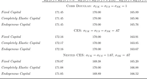
each pair of inputs is σU S=σU K = σSK = ₁₋1_ϑ. >From (7), factors receive their marginal

products and the wages under CES production reduce to:

w_S0(t) =ϑα(1₋β)LS(t)ϑ−1/Y (t) (21)

w0_U(t) =ϑ(1₋α)LU(t)ϑ−1/Y (t) (22)

whereY (t)is total output. Dividing (21) by (22), the ratio of the two wages, the instantaneous

college premium, is identical regardless of what we assume about the supply of capital.

Result 3 If the production function is CES, shocks ξ(t) and π(t) induce the same changes in

the instantaneous college premium if capital is fixed, perfectly elastic, or endogenously supplied.

Does this mean that the endogeneity of the capital supply is only relevant for determining

the wage level or the discounted college premiumSP _{if the elasticities of substitution between}

the inputs are not equal? No. First, the total levels of outputY (t) in (21) and (22) will differ

depending on what we assume about the nature of the capital supply. Hence, even if wage

each wage over time, the rate of return to capital less the natural rate of population growth, is

sensitive to what we assume about the supply elasticity of capital.

What we assume about capital supply does not affect the ratio between the two wages,

but does affect the ratio between their discounted values. Nonetheless, the ratio between the

present values of each stream of wages is likely to be close to each other when the elasticity

of substitution is constant, even if neither the levels of these wages nor the rate at which each

is discounted is the same. Indeed the lower the elasticity of substitution, the smaller the gap

between the rate of return to capital under free capital flows and endogenous capital supply,

and the smaller the difference in the discounted college premium.

6

Modelling the Impact of Immigration and Educational

At-tainment Over Time

Most of the empirical work that measures the performance of immigrants and their families

focuses on labor market outcomes–either the wages they command when they work, or their

rates of employment. Work by Chiswick (1978), (1986), Borjas (1985), (1987), (1992), and

Card, DiNardo, and Estes (2000) document the earnings of immigrants to the United States

and work by Altonji and Card (1991), Borjas et. al. (1997) and Johannsson et. al. (2003)

focus on employment. My focus here is on educational attainment as a proxy for labor market

skills (see Jasso, Rosensweig, and Smith (2000) for a discussion). Wages in the model derive

directly from that. In addition, I am interested in the educational attainment not only of

the immigrants themselves, but of their descendants. Recent empirical work on assimilation,

and more particularly on educational attainment in the second generation, includes Gang and

Zimmerman (2000), Riphahn (2003) (both study Germany), and van Ours and Veenman (2003)

(who study the Netherlands).

My focus here is on unskilled immigrants and their children. Immigrants with baccalaureate

degrees remain educated to the end of their lives, while only a small number of uneducated people

who arrive in North America, Australia or Western Europe as adults, subsequently complete

college. From Figure 2 we see that most of the points are above the 45◦ line, suggesting that

at least some of the children of unskilled immigrants do attend college. Indeed comparing the

educational outcomes of the different immigrant groups to the most convenient reference point–

the older generation of U.S. natives and the children of U.S. natives–there seems to be far more

upward mobility among the immigrants. Bauer and Riphahn (2004) observe a similar pattern

when comparing educational attainment among the native Swiss population with that of second

generation immigrants to Switzerland, using micro-level data that includes direct measurement

of parental education.

are clearly related, and yet we distinguish throughout between the two. In an economy without

assimilation, a surge of immigration, even if temporary, can permanently alter the distribution

between the two skill-types. By treating changes in the rates of immigration and changes in

the shares of the two skill types as distinct and separate shocks in (15), I distinguish between

the immediate impact of an immigrant group’s arrival, and its long-run affect on the economy

as the group’s members and their families either assimilate, or exceed the general population’s

rate of college completion.

To simplify the analysis, I will assume that changes in the rates of immigration begin at

time zero, lastT years and are constant over the entire period. The change in the overall rate of

immigration is defined as , and the increase in the overall population that results from the new

policy is eT ₋1. The share of skilled workers within the immigration surge is ΠS(T), and the

share of unskilled workers in the immigration surge is ΠU(T) = 1−ΠS(T). Beginning at time

Q, some of these workers, or their descendants, shift between the two categories. By timeV the

share of skilled workers within this population stabilizes at ΠS(V), and the share of unskilled

workers isΠU(V) = 1−ΠS(V). Define a set of dynamic perturbations:

πi(x, j) =

1 T ln

" 1 +

¡

eT ₋₁¢_Π i(j)

Pi(0)

#

U(T ₋x), i_∈{U, S_}, j _∈{T, V_}. (23)

where the unit step indicator function _U : _{R → {}0,1_} returns the value of one for all

num-bers greater than, or equal to zero, and the value zero for all numnum-bers less than zero. The

perturbations directly affect the ratio of skilled to unskilled workers in the economy:

λ(t, j) = η(0)³e R0t(πS(x,j)−πU(x,j))dx₋₁

´

, j_∈{T, V_}. (24)

The perturbation to the ratio of skilled to unskilled workersη(t)is the sum of two components:

ξ(t) =λ(t, T) + ·

(t₋Q)_U(t₋Q)₋(t₋V)_U(t₋V)

Q₋V

¸

(λ(V, V)₋λ(T, T)) (25)

We replace the perturbationsπi(t), i∈{U, S}in (15)—(20) withπi(t, T), i∈{U, S}.These

represent the actual perturbations to the rates of immigration, whereas the terms πi(x, V)

i_∈{U, S_} correspond to a counterfactual policy under which the shares of skilled and unskilled

households within the population of additional immigrants areΠS(V)and ΠU(V),in the short

run and not merely in the long run. Thefirst component in (25),λ(t, T),expresses the direct

cumulative effect of the actual changes in immigrationflows, andλ(V, V)expresses the long-run

effect of the additional immigration, after they have completed their shift from the initial rate

of college attainmentΠi(T)to the final rate Πi(V), i∈{U, S}.

The first component of ξ(t), λ(t, T), expresses the initial, direct effect of the immigration

surge on the composition of the work force from the moment the new immigration policy is

announced till time T, when the immigration surge has concluded. If λ(T, T) > 0, then the

and the immigrants initially raise the value of η(t). Ifλ(T, T)<0, the share of skilled workers

is lower, and the immigrants initially lower the value of η(t). The second component in (25)

expresses movements of the immigrants between the two skill categories and their effect on the

overall labor force composition between the periodsQ and V.

A few examples of possible time paths forη(t)will help illustrate the behavior of the model.

The left-hand panels of Figure 3 illustrate the evolution of η(t) following a surge in unskilled

immigration only, and the right-hand panels of Figure 3 illustrate the evolution ofη(t)following

a surge in skilled immigration. The black curves represent the behavior of η(t) if there is no

assimilation, the dark grey curves represent the behavior ofη(t)if all the immigrants assimilate,

and the light gray curves correspond to instances where the shares of skilled and unskilled workers

within the immigrant population reverse over time.

Suppose the skill composition of the workers in the immigration surge does not match the

prevailing composition of the host country, but neither the immigrants nor their descendants

switch between the two categories after they arrive. In this case Πi(V) = Πi(T), i∈ {U, S},

which implies λ(V, V) = λ(T, T). The second term in (25) is zero, the behavior of ξ(t) is

determined by λ(t, T), and η(t) either declines or increases until period T, and then remains

fixed at its new steady state value. Each set of black curves in Figure 3 corresponds to the

extreme sub-cases in which an immigration surge is uniformly composed of either unskilled

(left-hand side of Figure 3) or skilled (right-hand side of Figure 3) workers. Note that in each

column the black curves are identical for different values of Q and V, and serve as points of

reference.

Suppose the surge of additional immigrants initially upsets the balance between skilled and

unskilled workers in the labor force, but gradually, over the time period betweenQandV, these

immigrants assimilate until the shares of skilled and unskilled workers exactly mimics that of

the general population. Under this scenario Πi(V) =Πi(T) =Pi(0), i∈{U, S} and therefore

λ(V, V) = 0. Consider a surge in unskilled immigration. If the process of assimilation begins

immediately and ends soon after the last of the additional immigrants arrive (Panel a) of Figure

3), the dark grey curve barely declines below its initial value. In Panel c) assimilation begins

immediately, but the process lasts longer and the decline in η(t) is steeper.

Immigrants, or more likely their descendants, may not merely assimilate. As we see in

Figure 2, few of the women among Greek immigrants to the United States have college degrees,

but a disproportionate fraction of second-generation Greek-American women do. Similarly, the

value of η(t) may first decline because of a surge of unskilled immigration, but rise above its

initial value by time V. Similarly it is possible (though a good deal less likely) that a surge in

immigration may initially raise, but ultimately lower the value of η(t). If the value of Q is set

above T, then the value ofη(t) first behaves according to λ(t, T), before beginning its ascent

Figure 3: The time paths of η(t), the ratio of skilled to unskilled workers, for different degrees of assimilation following different influxes of skilled and unskilled immigrants.

0 T Q V t

hH0L

hH0L+elHT,TL

hH[L _{gLlHT,TL<0,T<Q}

PUHVL=1 PUHVL=PUH0L

PUHVL=0

0 T Q V

hH0L

hH0L+elHT,TL

hH[L _{hLlHT,TL>0,T<Q}

PSHVL=1

PSHVL=PSH0L

PSHVL=0

0 Q T V t

h_H0L

hH0L+elHT,TL

h_H[L _{eLlHT,TL<0,T>Q}

PUHVL=1 PUHVL=PUH0L

PUHVL=0

0 Q T V

h_H0L

hH0L+elHT,TL

h_H[L _{fLlHT,TL>0,T>Q}

PSHVL=1

PSHVL=PSH0L

PSHVL=0

0 T V t

hH0L

hH0L+elHT,TL

hH[L _{cLlHT,TL<0,Q=0,V>>T}

PUHVL=1 PUHVL=PUH0L

PUHVL=0

0 T V

hH0L

hH0L+elHT,TL

hH[L _{dLlHT,TL>0,Q=0,V>>T}

PSHVL=1

PSHVL=PSH0L

PSHVL=0

0 T V t

h_H0L

hH0L+elHT,TL

h_H[L _{aLlHT,TL<0,Q=0,V>T}

PUHVL=1 PUHVL=PUH0L

PUHVL=0

0 T V

h_H0L

hH0L+elHT,TL

h_H[L _{bLlHT,TL>0,Q=0,V>T}

PSHVL=1

PSHVL=PSH0L

Preferences, Technology and Factor Shares:

ρ=.0495 Matches average rate of return on capital of 5%.

δ =.061 Average rate of depreciation on capital: 1991-2000.†

α=.283 Average U.S. capital’s share of national income: 1991-2000.†

β=.482 Matches ratio of initial earnings.†‡§

Population:

n=.0067 Average U.S. natural rate of population growth: 1991-2000.‡

mS=mU=.0034 Average U.S. rate of net migration: 1991-2000.‡

κS=κU= 1 Immigrants arrive without physical capital.

PS(0)=.256 Population with college degrees.‡

d= 2.7 Ratio of initial earnings and wealth.

for households with/without college degrees.‡§

Table 1: Paramaterization of Baseline Model. †Bureau of Economic Analysis. ‡U.S. Census Bureau. §_{1998 Survey of Consumer Finances.}

Figure 3). However if the value of V is no longer zero, but below T, then the reversal in the

direction of η(t) begins at time Q(the light gray curves in Panel e) or Panel f) of Figure 3). If

Q=0, then as in Panels a), b), and c) the direction of η(t) may be completely determined by

the value ofΠi(V).

7

Parameterizing the Model

Between 1990 and 1999 the net rate of migration to the United States was just under 3.2 per

thousand. Although a much larger fraction of immigrants have less than nine years of schooling,

the percentage of the foreign-born with baccalaureate degrees closely matches that of the general

population–25.8% of foreign-born people in the United States over the age of 25 have college

degrees, as compared to 25.6% of the total U.S. population. For the initial stock of skilled

and unskilled workers we set PS(0) = .256 and PU(0) = .744, and set the steady state rates

of immigration for both skill types to mS = mU = .0032.13 If the rates of legal and illegal

immigration to the United States during the decade of the 1990’s carry forward, and the rate

of out migration continues to hold steady at one per thousand, foreign migration will augment

the U.S. population with close to ten million additional people over the course of this decade.

1 3_{At the high end, graduate education declines slightly with the degree of nativity: 9.7% of the foreign born}

have graduate degrees, as do 8.9% of natives with foreign-born parents, but only 8.2% of natives with native-born

parents. Grade school education rises more steeply with nativity–22.2% of the foreign-born and 10.1% of the

natives with foreign-born parents have less than nine grades of schooling (7.2% of the foreign-born have less than

five), against only 4.5% with less than nine grades among the native-born population with native parents (See

There is no readily available data on the financial assets or physical capital that new

immi-grants to the United States bring. Given the large gap in income between sending countries and

the United States, and the relative youth of most immigrants when they arrive, it is unlikely

that capital holdings for the typical immigrant, skilled or unskilled, approaches U.S. per-capita

capital holdings for either skill type. I setκS=κU = 1, which implies that afterfinancing their

move to the United States and setting up a household, immigrants have exhausted their savings.

I also assume that both types of workers supply the same amounts of labor and setlU =lS= 1.

The ratios of mean earnings and income for households, as well as individuals, with bachelor’s

degrees to those without, range from 2.13 to 2.71, as measured by the U.S. Census. The 1998

Survey of Consumer Finances reports on net wealth as well as income and earnings. The ratio

of mean earnings is 2.35, that of income is 2.3 while net wealth is 3.3. The gap between median

earnings and wealth is smaller–2.4 versus 3.06. In steady state, the ratio of capital held by

skilled and unskilled agents must be equal to the ratio of their wages. I choose an intermediate

number 2.7, and combine this with the 1991 to 2000 average share of capital in national income,

28.3%, to set the values of the parameters in the production function for different elasticities of

substitution.

Both the cross-country estimations of the nested CES production function (10) by Fallon

and Layard (1975) and Duffy et. al. (2004) and the time-series estimations using U.S. data by

Krussel et. al. (2000) and Swedish data by Lindquist (2003), find that the difference between

the values of the parametersϑ and υ in (10) is statistically significant–implying the existence

of the capital skill complementarities first postulated by Griliches (1969).

I simulate the baseline model settingϑ=.401andυ=₋.495in (10) to match the estimates

by Krusselet. al. (2000) (their distinction between skilled and unskilled workers based on college

education matches my own). These parameter values correspond to elasticities of substitution

between capital and unskilled laborσU K, and between skilled and unskilled laborσU S, that are

equal to ₁₋1_ϑ =1.67, and an elasticity of substitution between capital and skilled laborσSK equal

to ₁₋1_υ =.67.14 _{When ϑ is set equal to υ, the production function (10) becomes the standard}

CES function with three inputs, and when both approach the value of one in the limit we have

the Cobb-Douglas function.

1 4

The Allen Hicks partial elasticity of substitution between capital and unskilled labor, and between skilled

and unskilled labor are also equal to .67, but the Allen Hicks partial elasticity of substitution between capital

and skilled labor is 1 1−ϑ+

1

φSK

³

1 1−υ−

1 1−ϑ

´

8

A Twenty Year Surge in Immigration

8.1

Wage Levels

Comparing the period 1980-1989, and the period 1990-1999 in Figure 1, Panel b) the rate of net

international migration rose by just over .3 per thousand. In the next two sections I consider the

implications of an additional rise of a similar magnitude, that lasts for two decades. To begin

with, let us suppose that all the additional immigrants are people without college degrees. The

overall rate of immigration rises from 3.2 to 3.5, per thousand and the rate of immigration by

the unskilled rises to just over 3.6 per thousand.

How many additional people does such a rise in immigration imply? If present trends

continue, the United States will absorb about twenty million legal and illegal immigrants over

the course of a two decades, and fifteen million of them will not have Baccalaureate degrees.

The change considered here need not entail an increase in the number of legal immigrants alone.

A slight curtailment in enforcement efforts along the border could easily cause the number

of unskilled immigrants to rise by the additional seventy five thousand people per year (one

million-and-three-quarters over the course of twenty years) that we are considering here.

Consider first the effect of the policy change on each type of wages when assimilation does

not occur. Setting ΠS(T) = ΠS(V) = 0, and the elasticities of substitution in the production

function (10) σSK = .67, and σU K = 1.67, the surge of unskilled immigration produces a

permanent change in the skill composition of the work force, and generates the changes in the

wages of unskilled workers shown in the upper left-hand corner of Figure 4. The dotted lines

represent the impulse response in an economy with an inelastic supply of capital. Here, because

of the permanent dilution of the capital stock, the long-run response of unskilled wages, a drop

of just above .35% for the Nested CES production function, is twenty percent higher than the

long-run decline in wages if capital is either completely elastic or endogenously determined. By

contrast, the rise in skilled wages of over three-tenths of a percent if capital is elastic, in the

upper left-hand corner of Figure 5, is well over twice the rise in skilled wages if capital is fixed.

The impulse responses in Figures 4 and 5 are all relatively modest because they were

cal-culated for an economy in which the elasticity of substitution between the two types of labor

is high. If the elasticity of substitution between all the inputs is lower, the effect of

immigra-tion on both skilled and unskilled wages is larger. Setting all the elasticities of substituimmigra-tion to

two-thirds, the long-run drop in unskilled wages is close to nearly nine-tenths of a percent if

capital is fixed, and nearly sixth-tenths of a percent if capital is elastic. The long-run rise in

skilled wages is one-third of a percent if capital isfixed, and nearly twice that amount if capital

is elastic (see Figures 9 and 10 in the Appendix).

Whether or not there is free movement of capital, or if capital is elastically supplied but

the responses of wages is only a short-term phenomenon, and for the case of unskilled

immigra-tion, this difference is very small. In general, the response of wages if capital is endogenously

determined falls between two extremes, i.e., between the case where the capital supply grows at

an exogenous rate, and that where capital is perfectly elastic–but is much closer to the latter

than the former. Of course it must be emphasized that in the overlapping dynasties model there

is no representative consumer. Ensuring aggregability requires a logarithmic utility function,

and hence a relatively high degree of intertemporal elasticity of substitution in consumption. If

the elasticity of substitution were lower, the accumulation of capital would be slower, and the

short-term response of wages in the case of endogenously supplied capital would not be quite so

close to the responses generated by the model with perfectly elastic capital.

The upper right-hand graphs in Figures 4 and 5 illustrate the response of wages ifΠS(T) = 0

but ΠS(V) = PS(0) and PS(0) = .256. In the twenty-fifth year (Q=25), five years after the

immigration surge has ended, the descendants of these additional unskilled immigrants enter the

labor force. Of these new workers 25.6% are skilled, exactly mirroring the proportion of skilled

workers within the larger population. By year forty-five (V=25) this additional population

has completely assimilated. The arrival of these additional workers dilutes capital and causes

both skilled and unskilled wages to drop in the short run, but will not affect long-run wages

unless capital is inelastic. If capital supply is inelastic, unskilled wages drop by between a

third of a percent by year twenty (as in Figure 4), or just under nine-tenths of a percent

(as in the Appendix), depending on the elasticity of substitution. The drop is caused by the

combined effect of an increase in the relative share of unskilled workers in the labor force,

and the overall rise in the size of the labor force itself. In the long run, as the descendants

of immigrants assimilate, only the latter of these two effects remain, and the unskilled wage

recovers approximately half its short-term loss.

Wages for skilled workers initially climb, as the additional immigrants upset the balance

between skilled and unskilled workers. In each case, this change in the composition of the labor

force initially dominates the effects of capital dilution. If capital supply is completely elastic

or endogenous, the skilled wage also returns to its initial level, once the immigrants or their

descendants completely assimilate.

If capital is in fixed supply, the skilled wage initially rises but ultimately declines. If σSK

= .67, and σU K = 1.67, the wage is one-tenth of a percent higher by year twenty, but then

begins to gradually decline, until it is half a percent below where it was before the new policy

was initiated. If both elasticities of substitution are two-thirds, the wage initially rises by one

third but is ultimately four-tenths of a percent lower, and if both elasticities are one the wagefirst

rises by two-tenths of a percent and then by half a percent, until it is three-tenths of a percent

below its initial level (see Figures 9 and 10 in the Appendix). The greater the complementarity