City, University of London Institutional Repository
Citation
:
Cooper, E. S., Dissado, L. A. and Fothergill, J. (2005). Application ofthermoelectric aging models to polymeric insulation in cable geometry. IEEE Transactions on Dielectrics and Electrical Insulation, 12(1), pp. 1-10. doi: 10.1109/TDEI.2005.1394009
This is the unspecified version of the paper.
This version of the publication may differ from the final published
version.
Permanent repository link:
http://openaccess.city.ac.uk/1356/Link to published version
:
http://dx.doi.org/10.1109/TDEI.2005.1394009Copyright and reuse:
City Research Online aims to make research
outputs of City, University of London available to a wider audience.
Copyright and Moral Rights remain with the author(s) and/or copyright
holders. URLs from City Research Online may be freely distributed and
linked to.
Application of thermoelectric ageing models to
polymeric insulation in cable geometry
E. S. Cooper, L. A. Dissado*, J. C. Fothergill
University of Leicester
Leicester LE1 7RH
U.K.
Abstract
The life expressions of models of insulation ageing are functions of temperature and
field as well as material parameters. A methodology is presented that allows these
models to be applied to a cable geometry in which there is a radial variation of both
field and temperature. In this way material parameters can be extracted from cable
data. The methodology is illustrated using one such model and the parameters
deduced from cable failure distributions are compared with those obtained for thin
films. This comparison allows conclusions to be drawn about how the ageing process
affects specimens of the same material with different volumes.
Keywords
1. Introduction
Polymeric materials are used as electrical insulators in a wide range of industrial
applications, from thin films in capacitors to thick insulation layers in high voltage
power cables. In all cases the service life of the dielectric is of major commercial
interest and consequently a number of theoretical models have been developed with
the aim of relating the working lifetimes of dielectric polymers to the electrical and
thermal stress experienced. Current interest has focussed on physical theories
proposed by: by L.A. Dissado, G.C. Montanari and G. Mazzanti [1-4], T.J. Lewis, P.J.
Llewellyn, C.L. Griffiths, P.W. Sayers and S. Betteridge [5-13], J.P Crine and J.
Parpal [14,15], L. Simoni [16], and J. Artbauer [e.g. 17].
Ageing models such as those mentioned above generally result in a mathematical
expression that describes the lifetime of a specimen as a function of the electrical
stress, E, and temperature, T it experiences. Other factors related to material
properties are also involved. When the specimens under investigation are thin films
aged under spatially constant field and temperature conditions, fitting such
expressions to lifetime data and conversely predicting lifetimes using them is
relatively straightforward. However, in systems such as power cable insulation the
situation is more complex. The insulation of a power cable under load experiences a
radially varying temperature distribution due to Joule heating of the conductor
[18,19], as well as a radially varying electrical stress distribution, which will be
different for AC and DC applied voltages [18,19,20]. The difference in AC and DC
electrical stress profiles arises from the fact that in the AC case the stress profile is
temperature – at least for the range of temperatures typically experienced by cable
insulation. In the DC case the electrical stress is controlled by the conductivity, which
is strongly dependent on both temperature and stress, and this can lead to a situation
in which the field stress experienced by the insulation is not necessarily largest close
to the cable core. This effect is described briefly in the following sections. The radial
variation in E and T makes using the ageing models to either fit or predict lifetime
data in cable ageing experiments more difficult than in the thin film case.
In the first instance it may seem that all that is required to convert the life models to
cable geometry is to calculate the region where the electric field and temperature is
largest and then apply them to that region as a cylindrical shell. However such is not
the general case. For DC power cables in particular it cannot always be assumed that
the region where the temperature is highest is the region where the electric field is
highest [21]. In the second place the region at risk depends upon the physics of the
ageing process, for example in [1-4] this is assumed to be the region of highest space
charge concentration, in [5-13] it is assumed to be a layer of high electro-mechanical
stress, and in [15, 16] regions of free volume that allow high local currents. Finally
there are the material factors that are involved in ageing, such as the activation energy
for the process, the susceptibility of the local regions to the action of the field, and the
amount of local damage needed for imminent failure to be initiated. All of these may
be distributed in value [22]. There may also be radial differences in morphology that
will affect the factors controlling ageing. Sample ageing will take place most rapidly
in the region where the combined factors of temperature, field, and material properties
variations, and this cannot be restricted to a single shell but will have to involve the
whole of the cable.
In the following sections we describe a general methodology that allows ageing
models to be applied to cable geometry. In principle this methodology allows
prediction of cable lifetime using model parameterisation from thin films, however
the unknown volume dependence of the thin film parameters makes this procedure
impossible at present. Instead the method is used to derive parameter values
appropriate to the cable volume from cable failure data. This approach is illustrated
using the DMM [1-4] lifetime expression. In this work the method is applied to data
from ac ageing as this simplifies the calculation and was the only data available to the
authors in sufficient quantity to make an analysis feasible. The method is however,
equally applicable to ageing in a dc field provided that the difference in the radial
variation of the temperature and field is taken into account. The calculation is also
simplified by focussing upon the characteristic values of the parameters of the life
expression. These are derived and compared to those obtained for thin films and the
differences commented upon. Calculations that take account of the distribution in
value of the material parameters in order to fit the experimental life distributions [22]
will be reported at a later date.
2. Method
All theoretical models yield an expression for the lifetime in terms of temperature,
electric field and mechanistic parameters that may be dependent upon the material
and/or the electrode-material interface. In the case of cable insulation one or both of
electrode. The theoretical life expressions will therefore yield different thermoelectric
lifetimes depending on the radial location of the region considered. Some regions will
therefore reach the endpoint of ageing before others. In order to relate the theoretical
models to the service life of the cable, it is therefore necessary to decide upon the
condition under which the cable fails – i.e. whether it is necessary for the whole cable
to age to a defined end-point, or whether it is sufficient for only one region to reach
this degree of ageing. In the latter case cable failure will be initiated in the region that
has reached a critical level of ageing and rapidly proceed to completion. The
philosophy of the current ageing theories is in accord with the latter viewpoint and it
is therefore the one that we shall adopt here.
2.1 Shell model
The radial variation of temperature and electric field is allowed for by dividing the
cable insulation into a series of thin films within which temperature and field can be
considered constant. Each shell can therefore be assigned a lifetime using the theories
appropriate to thin films under uniform field and constant temperature.
Figure 1 shows a cable with a typical simple design, comprising a cylindrical core
covered in a layer of insulation. An example „shell‟ at radius ri is shown. Such shells
can be of equal thickness, or equal volume. None of the ageing models mentioned in
the introduction takes account of any of the spatial dimensions of the polymer
specimen, or those of the test electrodes. In fact, depending on the mechanisms of
ageing, at least one of these factors is likely to be important to the lifetime of a
polymer specimen. It is commonly assumed that ageing is a bulk process, in which
and this is discussed further in section 4.2. Considering shells of equal volume means
that the effect of volume on ageing will be the same for each, and this option is
therefore used here.
2.2 Radial dependence of E and T
The field and temperature experienced by each of the shells described above is a
function of the shell‟s radial position, ri. The temperature of a shell at radius ri can be
written as (see [18,19]):
i O i r R Th W T r T ln 2 )
( 1 (1)
where W is the power dissipated per unit length by the core under load and Th is the
combined thermal resistivity of the insulation and any outer layers. RO is the cross
sectional radius of the cable as shown in figure 1, and T1 is the temperature of the
outside of the cable –i.e. the ambient temperature.
Under AC conditions, the RMS electrical stress experienced by the same shell is e.g.
[20]: I O i i R R r V r E ln ) ( (2)
V is the voltage applied to the cable core, RO is as defined above and RI is the cross
sectional radius of the cable core. The above expression shows that in the AC case,
If a DC voltage is applied to the cable core, the electrical stress profile is more
complicated, and is given by [18,20]:
O I O O i i R R R R r V r E 1 ) ( 1 (3)
where all symbols have their previous meanings, and δ is given by
1 2 I O I O R R mV R R mV Th W a (4)
In equation 4, a and m are constants in equation (5) describing the resistivity, ρ of the
insulation in terms of electrical field, E and temperature T:
) exp( ) exp(
0 aT mE (5)
In equation (5) ρ0 is resistivity at T=0 and for vanishingly small E.
The expression for E(r) in the DC case leads to a situation in which the electrical field
strength may actually be largest at the outer edge of cable insulation systems for some
values of current [18,20,21].
2.3 Predicting Cable Lifetimes
temperature T(ri) and field E(ri) will therefore give the characteristic life of the shell if
its volume is the same as that of the specimens for which the parameters are derived.
The probability of survival to time t of the „i‟th shell is thus given by
i S
L t i
P ( ) exp (6)
where β is the time exponent of the Weibull distribution [23,24] that fits the thin
sample data. Of course an alternative distribution could be used if applicable. The
probability of survival of the whole cable is given by the joint probability of survival
of all the shells, under the assumption that a failure initiated in any one of them is
sufficient to fail the whole cable. This gives equation (7),
i S S
F P P i
P 1 1 ( ) (7)
The resulting failure distribution PF can be analysed to determine the characteristic
life of the whole cable and the failure time distribution [22]. There is however a
drawback to carrying through this approach. In general it will be difficult to equate
the shell volume to that of the specimens used in the parameterisation of the life
expression. If this is not possible the thin film parameterisation cannot be assumed to
apply to the cable shell, and in the absence of a measured or theoretical size
dependence the parameters cannot be modified appropriately. Of course equation (7)
could be taken to refer to a cable length small enough that the shell volumes are the
) (sec
) ( ) (sec )
( l tion
cable l S
S cable P tion
P (8)
where l(cable) is the cable length and l(section) is the section length as defined above.
Even this approach is only possible if the volume of the thin film samples is known
and we assume that the size effect is in fact a volume effect rather than one related to
electrode area or sample thickness. In the light of these difficulties we have adopted a
different approach described in the next section.
2.4 Parameterising life expressions from cable data
In this approach we relate observed cable data to life expression parameters
appropriate to the complete insulation volume of the cable. In this section we shall
denote the characteristic lifetime of the cable by B63, which is defined as the time at
which a fraction (1-e-1) equal to 63.2% of the samples have failed. The value of B63
for cables can be obtained from their lifetime distribution in exactly the same way as
for thin films. However fitting it to the theoretical life expressions is more complex
than for thin films. In the thin film case it is only necessary to fit the expressions to a
set of lines giving the T and E dependence of the characteristic life (e.g. [1-4]). In the
case of cables each of the shell life expressions is a function of the model parameters
and a different E and T value depending on its radial position. To find values for the
parameters relevant to a particular set of cable specimens, the shell expressions must
be combined, and fitted to experimental ageing data. A method for combining N shell
lifetime expressions in order to fit them to the characteristic lifetime at each
It is assumed that in cable insulation of volume VC made up of N shells, failure in any
one of the shells will cause the whole insulation to fail. In this case, the following
equation links the probability of survival of the whole insulation to the probability of
survival of N constituent shells.
N
i
i S
S C P S
P 1 ) ( ) ( (9)
Here, PS(C) is the probability of survival at a given time of the whole insulation. PS(S)
is the probability of survival of a constituent shell. Each shell has a volume
VS=VC/N.
The time to failure distributions resulting from ageing tests on polymer specimens are
commonly assumed to be Weibull distributions with a shape parameter, , which is
characteristic of the ageing process e.g. [22-24]. This assumption is reasonable if a
failure in polymeric specimens can be assigned to the „weakest‟ region of polymer,
where ageing proceeds faster than in any other. Assuming, therefore, that PS(C) and
PS(S) are Weibull distributions with the same β value, they are given by e.g.[24].
63
exp
)
(
B
t
C
PS
(10) iL
t
S
PS
(
)
exp
(11)Here t is time, B63 is the characteristic lifetime of a set of cables aged under the same
experimental conditions and Li is the characteristic lifetime of a set of shells of
parameter of the time-to-failure distribution from the cable ageing experiments, and in
equation (11) is the shape parameter of the distribution of the shell times-to-failure. It
has been assumed that the values of in the above equations are the same. This may
not necessarily be the case depending upon the origin of β [22], but the introduction
of a difference between its value for the shell and the cable would require more
knowledge than we have at present and hence is not justified.
By substituting equations (10) and (11) into equation (9), an expression can be
derived for the characteristic lifetime of cable insulation, B63 in terms of the
characteristic lifetimes, Li, of a set of insulation shells.
i Li
B
1 63
1
(12)
In this case, B63 is the characteristic lifetime of a cable set, and Li can be replaced
with an expression for the lifetime of the „i‟th shell. Equation (10) can therefore be
used to fit the chosen expression to experimental B63 values in order to obtain
parameter values.
The parameter values obtained from fitting equation (12) will necessarily depend on
the volume of the cable insulation through B63, just as in the case of thin films the
parameters depend upon the film volume [24]. However, using equation (12) means
that the parameter values must also have a dependence on the shell volume (or
equivalently a dependence on N), since the probabilities PS(S) in equation (9) are
volume dependent. Parameters that depend on both VC and N have the disadvantage
the parameters from film experiments will only depend on the total film insulation
volume – equivalent to VC for cables.
To get parameter values from cable experiments that only depend on VC, it is
necessary to „scale up‟ the probability of failure of each shell to the total insulation
volume. In other words, it is necessary to determine an expression for the probability
of failure that each shell would have if it had the volume of the whole insulation. This
is equivalent to the probability of failure of a shell, with volume VC, comprising N
shells each experiencing the same E and T conditions. This can be obtained using an
expression of the same form as equation (9):
N
i
i S
S SS P S
P
1 ) ( )
( (13)
Here PS(SS) is the probability of survival of the scaled up shell with volume VC, and
PS(S) is the probability of survival of the original shell. Since each value of PS(S) is
the same in this case, this gives
N i S i
S SS P S
P ( ) ( ) (14)
Taking the product of the PS(SS) values over all the shells now gives the probability
of survival of a volume of insulation N times bigger than VC – i.e.
N
i
i S
S NC P SS
P 1 ) ( ) ( (15)
Substituting for PS(SS) from equation (14) then gives
N
i
N i S
S NC P S
PS(NC) is the probability of survival of a cable specimen with a volume N times
bigger than VC. To get the probability of survival of cable insulation of volume VC
(i.e. of the total cable insulation), equation (14) can be used together with equation
(16) to give
N N i i S N S
S C P NC P SS
P 1 1 1 ) ( ) ( )
( (17)
Here PS(C) is the probability of survival of the cable. Using this equation, and
assuming again that the probabilities of survival are all Weibull distributions with the
same shape parameter, the following equation is derived
i Li
N B 1 1 63 1 (18)
Li is now an expression for the lifetime of a scaled up shell – i.e. an expression for the
lifetime that a shell would have if it had volume VC. It is important to note that Li in
expression (18) has a different meaning to Li in equation (12), despite the fact that
they both relate to the same life expression. Fitting of expression (12) to data results
in model parameter values that depend on N, whereas using equation (18) gives
parameter values that are independent of N and depend only on the total volume of
3. Application to data
In order to illustrate the methodology described in section2 we will apply it to a
specific life expression, namely that of the DMM model [1-4]. This model gives the
life, Li, of the „i‟th shell, at temperature T(ri) and field E(ri) in the form
) ( 2 ) ( cosh * ln ) ( 2 ) ( exp exp ) ( 2 4 4 i b i d d eq eq i b i d dk d i i r T r E C K A A A r T r E C H k S r kT h L (19)
The factor Aeq is defined through expression (20),
)] ( / ) exp[ 1 1
)
(
(
K
C
E
r
4r
A
i b d d eq T i (20)There are therefore only six nominally independent parameters in the life expression,
b, A*, Hdk, Sd, Kd and Cd. This expression is based on the concept that the energy
stored in local concentrations of space charge causes a local deformation of the
polymer to exceed a critical level at which free volume generation and nano-void
coalescence occurs. Failure is then rapidly brought about by partial discharging
leading to electrical trees and connection of the void population. The polymer chains
are conceived as possessing alternative configurations with the one corresponding to
the deformation being energetically unfavourable with respect to the other. The
energy difference is Kd (in units of Kelvin). The „reaction‟ from one configuration to
the other requires a free energy barrier to be exceeded, composed of an activation
absence of the space charge produced by the applied field E, the fraction of local
configurations in the „deformed‟ state will reach an equilibrium value Aeq. The space
charge concentration has been assumed to be proportional to a power b of the applied
electric field, (i.e. local charge = qloc Eb) [1-4] and to modify the energy barrier and
energy difference between the alternative configurations via an electro-mechanical
energy leading to the energy term CdE4b in the above expressions. It is assumed that
life is terminated when the fraction of configurations in the „deformed‟ state reaches a
level sufficient for coalescence into voids, starting from an initial non-equilibrium
state corresponding to an unaged material. This critical fraction is denoted by A*. The
reader is referred to references [1-4] for more detail. Each of the parameters are
expected to be essentially independent of temperature, and the role played by the local
temperature in the life expression is explicitly defined via equation (19). In AC fields
Sd and Hdk become frequency dependent [4], whereas in DC fields Sd can be taken to
be zero [4] thereby reducing the number of parameters to five.
This expression was chosen here because the parameter values for a number of
materials are available in the literature [1-4]. In addition the expression exhibits all the
basic features present in the other models – i.e. an activation free energy that must in
general involve two parameters, a field effect term involving a composite parameter,
here Cd, and a field power term usually assumed to have the value b=0.5. The other
features A* and Kd lead to a field threshold, which is a controversial feature that is
also found in [5]. The choice of expression encompasses all possible features and also
poses a challenge to the method, and for this reason we have chosen to use it as an
example to illustrate the application of the method. However in the context of cable
geometry the chosen life model can be simplified by using either a known or
relating space charge concentration to the local field and hence remove „b‟ from the
list of parameters. It should be noted however, that our choice of model was made
strictly for convenience in testing and that the method can be applied to any life
expression and is not restricted to the model chosen.
3.1 Details of fitting method
Data used
The method described in section 2 was used to fit the DMM life expression to
experimental data from cable ageing experiments carried out for BICC Cables Ltd
(now owned by Pirelli Cables Ltd.) [26]. Cables insulated with extruded XLPE of
thickness 4.4mm were aged under nine different experimental conditions. Twelve
cables were aged under each condition, and the tests were stopped after eight cables
had failed. A Weibull analysis applicable to singly censored data was therefore
carried out [23], resulting in B63 and β values for each of the nine experimental
conditions.
The cables were 15kV medium rated cables, with aluminium cores and values of RI
and RO of 5.9mm and 10.3 mm respectively. They were all 9.14m long. Cables were
aged at temperatures of 60°C, 75°C and 90°C and applied AC r.m.s. voltages of
34.6kV, 26kV and 17.3kV. The cables also contained thin semicon layers between the
core and the insulation, though these were ignored for the purposes of the fitting. This
is justifiable here, since the only effect of an extra layer would be to change the mean
thermal and electrical resistivities of the insulation/semicon layer and in all cases the
temperature was assumed constant across the insulation. There was therefore no
temperature gradient across the insulation – only an AC-type field gradient, which is
independent of both the electrical and thermal resistivity of the insulating layer as
shown in equation (2).
Error function
In order to fit experimental data to the DMM model, the following error function,
representing the difference between experimental data and the model predictions, was
minimised to find optimal DMM parameter values in Li
J
J
i i
J
r L
N B
2 1
) (
1 ln
) 63
ln( (21)
Above, J is the number of B63 values available. For each B63 value, the error
function takes the difference between the log of the B63 value and the log of the
hypothesised cable lifetime expression as in equation (19). The squares of the
differences are summed over all experimental conditions to give the final error value
for the whole data set. Natural logarithms are used in the error function due to the
extreme non-linearity of the DMM equation. The square of the differences is used to
avoid fits where the fit is good for most B63 values but very poor in one or two cases.
Equation (21) was minimised using a grid search method implemented using a
Values of N and β
The number of shells used in this fitting, N, was 100. This value was chosen for
several reasons. Firstly, N=100 corresponds to a situation where the thickest shells in
the cable are roughly the same thickness as the PET films for which the DMM model
has been previously shown to give a good fit [3]. Since the models were originally
applied to thin films, ensuring that the shells are of a similar thickness ensures that the
applicability of the expression demonstrated on thin films is retained. Secondly, N
was chosen to be high enough to give as good a fit as possible to the data. Since the N
dependence of the model parameters is eliminated in the fitting function, the only
effect of increasing N should be to increase the quality of the fits due simply to an
improved accuracy in the discrete representation of a continuous system. This effect
was found to reach saturation at a value of N of approximately 100. The third criterion
for a value of N is that it cannot be too large that the computation takes too much
time.
A value for β also had to be chosen, since the error function requires only one value
of beta. Each experimental condition yields its own value of β, and for the data used
here the β values ranged from 2.4 to 8.5 – each with fairly wide confidence limits. We
have assumed that each of these values is the same for each cable set so long as the
ageing process is the same, so an average of all the β values was used. This average
was weighted towards the smaller end, since the highest β was much higher than the
other values and was therefore deemed atypical.
The results obtained from fitting the DMM model to cable data as outlined above are
shown in figure 2.
In figure 2, the y-axis represents time in seconds, and the x-axis shows applied RMS
voltage in kV. B63 values from each of the nine conditions under which cables were
aged are shown as crosses, circles and triangles corresponding to tests at 363K, 348K
and 333K respectively. The 90% confidence limits for each B63 are shown as error
bars. Each of the lines in figure 2 represents the lifetime predicted by the DMM model
using the method described above. Each line shows predicted lifetime as a function of
applied voltage at a temperature corresponding to one of the ageing temperatures. The
lines show voltage threshold behaviour – i.e. below a threshold voltage, cables are
predicted to have an infinite life. However, the cable lifetime only becomes infinite if
the field and temperature experienced everywhere in the insulation – i.e. by each of
the constituent shells - is below the threshold for the material.
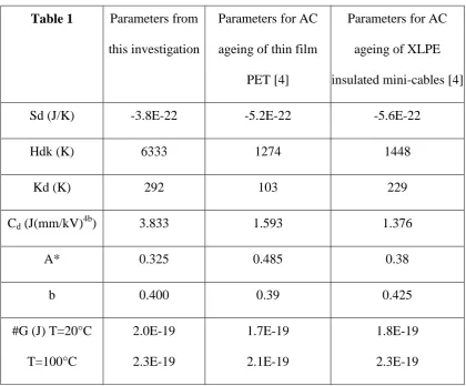
The parameter values used to obtain the fits shown in figure 2 are given in table 1,
along with the parameters from fitting to life data from other types of polymer
specimen.
In the FORTRAN grid search used here, the DMM parameters were allowed to vary
over wide ranges. The magnitudes of the model parameters obtained are nevertheless
all similar in magnitude to those obtained in previous fittings to AC ageing data of
XLPE mini-cables and PET thin films.
The fit in figure 2 can be seen to be good, with the predicted lifetimes being within
the 90% confidence limits of the experimental data for four out of the nine conditions.
This is a good fit considering the assumptions involved in the derivation of the fitting
method. The most significant of these assumptions is the way that the electrical field
strength is used in the method – firstly the electric field in each shell is calculated on
the basis of simplifying assumptions giving equation (2) and then this value is used in
the DMM model in another assumed relationship describing the amount of charge in
the material in terms of the local macroscopic field.
4.2 Parameter values – volume considerations
The magnitudes of the model parameters obtained are similar in magnitude to those
obtained in previous fittings to AC ageing data. This suggests that the cable fitting
method works well, and supports the contention that the ageing process is the same
for each of the materials studied.
The parameters in table 1 were obtained from fits to AC ageing data involving very
different specimen types. In this investigation, the cables were insulated with XLPE
with a volume of 2x10⁻³m3 and a thickness of 4.4mm. The mini-cables for which
parameter values are quoted had an insulation thickness of 1.5mm, and a volume of
approximately 3x10⁻⁶m3. The volume of the PET films is not known, but the thickness
of each was 50x10-6mm – implying a volume many times smaller than in either of the
cable cases.
Any dependence of specimen lifetime on volume must be reflected in the magnitudes
different volumes. The question as to how the specimen volume affects parameter
values in table 1, however, is not clear, since the parameters obtained are all for
different materials, as well as for different volumes. This is true even of the XLPE
cables evaluated here and the XLPE insulated mini-cables, since the XLPE was made
by different cable manufacturers in each case, and there are therefore likely to be
significant differences in composition between the two. It is therefore not possible to
separate out differences in parameter values due to volume, from differences due to
material morphology and chemical composition. The volume of insulation of the
cables used here, however, is considerably larger than in the other two cases – almost
700 times larger than the mini-cable insulation, and likely to be much larger again
than the PET films.
In spite of the material differences it is possible to use the parameter sets of table 1 to
speculate as to which of the DMM model parameter values might be affected by
volume. The common assumption that a larger volume of insulation will fail faster
than a smaller volume under the same conditions is essentially based on a statistical
argument (see for example [22,23]), i.e. bigger volumes give a greater preponderance
of sites susceptible to ageing and hence a bigger likelihood of the existence of highly
susceptible sites.
In the DMM models these sites are characterised by polymer moieties that can trap
charge and respond to the trapped charge by surmounting an energy barrier to an
alternative conformation corresponding to a local deformation. The influence of the
local space charge is to both accelerate the local changes and to stabilise a more
equilibrium in its absence. When the distortion exceeds a critical level it is assumed to
initiate a rapid failure process. Differences in the parameter sets obtained for cable
data as compared to the other two sets, particularly the mini-cables, may therefore
relate to a greater severity of the most susceptible sites.
Since the temperature is constant across the radius of the cable in the samples whose
failure data has been analysed (see section 3.1), a characteristic free energy barrier #G
(=Hdk-TSd) can be defined as for the thin film samples. As shown in Table 1 its value
is actually very similar for all of the three systems, however it is clear that the
component of the barrier arising from the activation enthalpy is greater in the
full-scale cables than in the other two cases. This means that ageing is much more
sensitive to temperature in the present cable data than for the other two systems. The
changes in barrier factors Hdk and Sd cannot be regarded as a volume effect as we
would expect larger volumes to lead to more susceptible sites, with smaller #G, over
the temperature range experienced by the cable. It should be noted that the value of
the activation entropy, Sd, is negative. This corresponds to a reaction in which the
ground state is more configurationally disordered than the barrier state through which
the reactants move to the product state. In this kind of reaction we can picture the
reacting moieties having to adopt specific orientations and bond angles in order to
achieve passage through the barrier. This requires work to be done on the group of
entities that have to pass through the barrier. The similarity in #G values appears to be
an instance of a compensation law and is also found for the ageing of PET films [1-4],
where #G is found to be the same in DC and AC ageing over the temperature range
measured. It is possible to speculate that this result indicates that the basic features of
changes with frequency and morphology. More specifically it would appear that as
the amount of ordering required to enter the barrier state becomes smaller (i.e. Sd
moves closer to zero) the system is forced to surmount a higher enthalpy barrier, i.e.
the disordered state has a large enthalpy barrier but ordering allows reaction via a
smaller entropy barrier at the expense of the free energy required for the ordering.
It is possible that the parameter A* may be affected by volume. A* is the fraction of
moieties that must be involved in deformation for breakdown to occur in any localised
area. It seems likely that this fraction might vary from region to region of the
specimen. This means that in a larger volume of polymer there may be an increased
likelihood of finding regions where fewer moieties need to be involved for breakdown
to be initiated. As a result, a specimen with a larger volume will require the
conversion of fewer moieties to initiate failure, and consequently a smaller local
energy concentration will be required. The differences in characteristic A* shown in
table 1 seem to support the hypothesis that the specimens with larger volumes require
fewer moieties to be converted, and therefore lower energy concentration, to initiate
breakdown. Larger volumes would therefore experience a reduction in lifetime under
a given condition.
Cd and b describe the effect of a field on the barrier to ageing, #G. On the application
of an electrical field of magnitude E, #G is reduced by an amount equal to CdE4b, and
this acts to accelerate the ageing reaction. Large values of Cd and b for a set of
specimens therefore indicate that the ageing reaction is accelerated strongly by the
electrical field. In addition, this field dependent energy helps to stabilise the state of
achievement of sufficient deformation to initiate failure. A greater volume of polymer
is more likely to contain sites at which this is the case – i.e. sites at which the field can
have a strong influence on the ageing process. In the DMM model such sites will be
those that have greater ability to trap charge and store electro-mechanical energy.
They may therefore be sites that have a bigger electrostriction coefficient than the
average for the specimen. Such sites may also (or instead) have a smaller bulk
modulus or relative permittivity than average. Microscopic variations in macroscopic
material characteristics such as these seem very likely, which makes these two
parameters likely to have a volume dependency. The data in table 1 seems to support
this to some extent, with the largest polymer volume showing by far the largest values
of Cd. The values of b are all quite similar, however, with no observable pattern with
volume. Overall, the CdE4b term for fields from 0 to 20kV/mm is always largest for
the XLPE cable parameters. The same term is larger for the mini-cables than for the
thin films for all fields above about 3kV/mm, but below this field the values are very
similar. These parameters are also likely to be strongly material dependent, however,
so this is by no means conclusive.
4.3 Relationship to Space Charge
The DMM ageing theory differs from the other models [5-14] in ascribing the ageing
to energy (electromechanical) concentration produced by trapped space charges. The
local energy is proportional to either the 4th power of the space charge field or its
square depending upon whether or not the local centre was assumed to behave as a
region with macroscopic properties or as an irreducible volume element with
atomistic/molecular properties [27]. The relationship to the known applied field was
The physics behind the model [1] therefore allows the possibility that a direct
measurement of space charge could be used instead of estimation of E(ri). This has the
benefit of eliminating the exponent b as a parameter, since the local space charge field
can be taken to be proportional to the space charge density. The effect of local field
would still be expressed through a parameter like Cd. One drawback to this course of
action is that trapped charges may be present though their net value may be zero. The
energy concentration and local field would still exist on the atomistic scale even
though the measured space charge would be zero. Secondly, the divergence of the
applied Laplacian field in cables would also yield an electromechanical energy
concentration [5] that would have to be added to the atomistic value. In order to
pursue this approach space charge measurements would have to be taken during
ageing and this information is not yet available.
5. Conclusions
The radial variation of temperature and electric field experienced in cable geometry
can be included in an ageing theory by means of a shell approach. The methodology
can be applied to any ageing theory and can, in principle, be used to predict cable
lifetimes from thin film experiments. In practice it is better suited to investigating the
volume dependence of ageing parameters.
The methodology has been applied to the life expression of the DMM model, which
was found to fit the data very well. It was shown that values of the A* and Cd
parameters correspond to a characteristic centre that is more susceptible to ageing, as
activation enthalpy component was bigger, It therefore seems possible to conclude
that the larger cable contains centres that require less energy concentration to achieve
the initiation of failure, that the centres are more susceptible to the affect of an
electrical field, but that the barrier to the ageing reaction involves different routes
REFERENCES
[1] L.A. Dissado, G. Mazzanti, G.C. Montanari, „The Incorporation of Space Charge
Degradation in the Life Model for Electrical Insulating Materials‟, IEEE Transactions
on Dielectrics and Electrical Insulation, Vol. 2, No 6, pp1147-1158, 1995.
[2] L.A. Dissado, G. Mazzanti, G.C. Montanari, „The Role of Trapped Space Charges
in the Electrical Aging of Insulating Materials‟, IEEE Transactions on Dielectrics and
Electrical Insulation Vol. 4, No 5, pp496-506, 1997
[3] L.A. Dissado, G. Mazzanti, G.C. Montanari, „Discussion of space-charge life
model features in dc and ac electrical aging of polymeric materials‟, Annual Report
CEIDP, pp36-40, 1997
[4] G. Mazzanti, G.C Montanari, L.A. Dissado, „A Space-charge Life Model for ac
Electrical Aging of Polymers‟, IEEE Transactions on Dielectrics and Electrical
Insulation, Vol. 6, No 6, pp864-875, 1999.
[5] T.J. Lewis, J.P. Llewellyn, M.J. van der Sluijs, J. Freestone, R.N. Hampton, „A
new model for Electrical Ageing and Breakdown in Dielectrics‟, IEE DMMA, Conf
Pub No 430, pp.220-224, 1996
[6] T.J. Lewis, „Ageing – A Perspective‟, IEEE Electrical Insulation Magazine, vol.
[7] T.J. Lewis, J.P. Llewellyn, M.J. van der Sluijs, „Electrokinetic properties of
metal-dielectric interfaces‟, IEE Proceedings-A, Vol. 140, No 5, pp.385-392, September
1993
[8] T.J. Lewis, J.P. Llewellyn, M.J. van der Sluijs, „Electrically induced mechanical
Strain in Insulating Dielectrics‟, IEEE Annual report CEIDP, pp 328-333, 1994.
[9] T.J. Lewis, J.P. Llewellyn, M.J. van der Sluijs, J. Freestone, R.N. Hampton,
„Electromechanical Effects in XLPE Cable Models‟, Proc.5th ICSD, (IEEE Pub.
95CH3476-9), pp. 269-273, 1995
[10] P. Connor, J.P. Jones, J.P Llewellyn and T.J. Lewis, „Electric Field-Induced
Viscoelastic Changes in Insulating Polymer Films‟, Ann. Rep. CEIDP, pp27-30, 1998
[11] C.L. Griffiths, J.Freestone and R.N. Hampton, „Thermoelectric Aging of Cable
Grade XLPE‟, Proc. IEEE ISEI, pp.578-582, 1998.
[12] P.W. Sayers, T.J. Lewis, J.P Llewellyn and C.L. Griffiths „Investigation of the
Structural Changes in LDPE and XLPE Induced by high Electrical Stress‟, IEE
DMMA, Conf Pub No 473, pp. 403-407, 2000
[13] C.L. Griffiths, S. Betteridge, J.P. Llewellyn and T.J. Lewis, „The Importance of
Mechanical Properties for Increasing the Electrical Endurance of Polymeric
[14] J.L. Parpal, J.P. Crine and C. Dang, „Electrical Ageing of Extruded Dielectric
Cables – a physical model‟, IEEE Transactions on Dielectrics and Electrical
Insulation, Vol. 4, No 2, pp 197-209, 1997
[15] J.P. Crine, „A Molecular Model to Evaluate the Impact of Aging on Space
Charges in Polymer Dielectrics‟, IEEE Transactions on Dielectrics and Electrical
Insulation, Vol. 4, No 5, pp487-495, 1997
[16] L. Simoni, „A general approach to the endurance of electrical insulation under
temperature and voltage‟, IEEE Transactions on Electrical Insulation, Vol. EI-16, No
4, pp277-289, 1981
[17] J. Artbauer, „Electric strength of Polymers‟, J.Phys. D: Appl. Phys., vol. 29, pp.
446-456, 1996
[18] C.K. Eoll, „Theory of Stress Distribution in Insulation of High-Voltage DC
Cables: Part 1‟, IEEE Trans EI Vol. E1-10, No. 1, pp.27-35, 1975
[19] The Development of a High Voltage DC Cable‟ Prepared by The Okonite
Company. EPRI EL-606 Project 7818.
[20] Edited by G.F. Moore, „BICC Electrical Cables Handbook‟, Blackwell Science
[21] S.A.Boggs, D.H.Damon, J.Hjerrild, J.Holboll, and M.Henriksen, “Effect of
insulation properties on the field grading of solid dielectric DC Cable”, IEEE Trans.
PD., vol. 16, pp456-461, 2001
[22] L. A. Dissado, “Predicting electrical breakdown in Polymeric Insulators, From
Deterministic mechanisms to Failure Statistics”, IEEE Trans DEI, vol.5, pp860-875,
2002
[23] J.C. Fothergill, IEEE Draft Standard P930: 'IEEE Guide for the statistical
analysis of electrical insulation breakdown data'
[24] J.C. Fothergill and L.A. Dissado, „Electrical degradation and breakdown in
polymers‟ P. Peregrinus for IEE, London, ISBN: 0 86341 196 7, 1992
[25] V. M. Morton and A Stannett, „Volume dependence of electric field strength of
polymers‟. Proc. IEEE, vol 115, pp1857, 1968
[26] BICC company report „Analysis of Accelerated Ageing Tests On Extruded
XLPE and EPR Power Cables Carried Out By EPRI at the Marshall Technology
[27] L.A.Dissado, G.Mazzanti, G.C.Montanari, „Elemental Strain and trapped space
charge in thermoelectric ageing of insulating materials. Life modelling‟, IEEE Trans
BIOGRAPHIES
Elizabeth Cooper
Elizabeth Cooper was born in the UK in 1976 and gained a degree in Physics with Astrophysics from the University of Leicester in 1999. In 2002 she received a PhD, also from the University of Leicester. She currently works with Professors Dissado and Fothergill in the high voltage laboratory of the engineering department at Leicester, researching the physical processes relevant to charge movement in the insulation of high voltage DC power cables.
Len A Dissado (Senior Member since 1996)
John C Fothergill (Senior Member since 1995)
Professor Fothergill was born in Malta in 1953. He graduated from the University of Wales, Bangor, in 1975 with a Batchelor‟s degree in Electronics. He continued at the same institution, working with Pethig and Lewis, gaining a Master‟s degree in
Table and Figure captions
Table 1 – Parameter values from fitting the DMM model to data. #G is the activation
free energy (=Hdk-TSd) at the temperatures quoted.
Figure 1 – Typical coaxial cable geometry with an example shell shown at radius ri
1
1
Application of thermoelectric ageing models to polymeric insulation in cable geometry
[image:36.595.89.510.98.446.2]ES Cooper, LA Dissado, JC Fothergill 27th May 2003
Table 1 Parameters from
this investigation
Parameters for AC
ageing of thin film
PET [4]
Parameters for AC
ageing of XLPE
insulated mini-cables [4]
Sd (J/K) -3.8E-22 -5.2E-22 -5.6E-22
Hdk (K) 6333 1274 1448
Kd (K) 292 103 229
Cd (J(mm/kV)4b) 3.833 1.593 1.376
A* 0.325 0.485 0.38
b 0.400 0.39 0.425
#G (J) T=20°C
T=100°C
2.0E-19
2.3E-19
1.7E-19
2.1E-19
1.8E-19
2
2
Application of thermoelectric ageing models to polymeric insulation in cable geometry
ES Cooper, LA Dissado, JC Fothergill 27th May 2003
Figure 1
RO Thickness
of cylindrical
shell ~0
RI
3
3
Application of thermoelectric ageing models to polymeric insulation in cable geometry
ES Cooper, LA Dissado, JC Fothergill 27th May 2003
Lifelines with Experimental Data
1.E+06 1.E+07 1.E+08 1.E+09
15 20 25 30 35
Voltage (kV)
L
if
e
(
s
)