A bounded upwinding scheme for computing convection-dominated transport problems

A bounded upwinding scheme for computing convection-dominated

transport problems

V.G. Ferreira

a,⇑

_{, R.A.B. de Queiroz}

a

_{, G.A.B. Lima}

a

_{, R.G. Cuenca}

a

_{, C.M. Oishi}

b

_{, J.L.F. Azevedo}

c

_{, S. McKee}

d a

Departamento de Matemática Aplicada e Estatı´stica, Instituto de Ciências Matemáticas e de Computação – USP, São Carlos, SP, Brazil b

Departamento de Matemática, Universidade Estadual Júlio de Mesquita Filho – UNESP, Presidente Prudente, SP, Brazil c

Instituto de Aeronautica e Espaço, CTA/IAE/ALA, São José dos Campos, SP, Brazil d

Department of Mathematics and Statistics, University of Strathclyde, Glasgow, UK

a r t i c l e

i n f o

Article history:

Received 20 April 2009

Received in revised form 26 September 2011

Accepted 27 December 2011 Available online 10 January 2012

Keywords:

Numerical simulation CBC/TVD stability High resolution Upwinding

Monotonic interpolation Finite difference Convection modeling Boundedness

a b s t r a c t

A practical high resolution upwind differencing scheme for the numerical solution of convection-domi-nated transport problems is presented. The scheme is based on TVD and CBC stability criteria and is implemented in the context of the finite difference methodology. The performance of the scheme is investigated by solving the 1D/2D scalar advection equations, 1D inviscid Burgers’ equation, 1D scalar convection–diffusion equation, 1D/2D compressible Euler’s equations, and 2D incompressible Navier– Stokes equations. The numerical results displayed good agreement with other existing numerical and experimental data.

Ó2012 Elsevier Ltd. All rights reserved.

1. Introduction

The development of fast, reliable and accurate numerical approximations for the convection terms of hyperbolic conserva-tion laws and transport equaconserva-tions in fluid dynamics has presented a continuing challenge. The most frustrating obstacle has been the attempt to prevent the unbounded growth of the unphysical spa-tial oscillations in the vicinity of sharp changes in gradients, or jump discontinuities. It is also essential that certain transport vari-ables remain bounded within physical limiting values. For exam-ple, the fluid depth in shallow water flows, the mixture fraction of reacting flows, the kinetic energy in turbulent flows, or species concentration all cannot fall below zero. Previous studies by Smith and Hutton[54](see also van Albada et al.[64]and van Leer[69]) have shown that upwinding schemes may produce nonphysical results when boundedness is not preserved.

In order to obtain stable, bounded and physically plausible

solu-tions, the classical first order upwind (FOU) difference scheme[21]

– or the hybrid central upwind (HCU)[48,58]– is often adopted.

However, this scheme is generally unsuitable for applications involving long time evolution of complex flows (unless extremely fine meshes are employed), mainly because extrema can become ‘‘clipped’’ and numerical dissipation (even spatial derivatives) can become dominant (see Refs. [13,46,59]).

The cure for this has been to use conventional schemes, such as

central differences (CDs), second-order upwind (SOU) [70], and

quadratic-upstream interpolation for convective kinematics

(QUICK)[39](or its related QUICK with estimated streamline terms

(QUICKEST)[41]), to name just a few. However, under highly

con-vective conditions, these schemes also inevitably generate

spuri-ous numerical (or non-monotonic) oscillations (wild [17] or

parasitic solutions[25]) and instabilities in regions where the con-vected variables experience discontinuities.

To overcome these defects, a number of monotonic high-order upwind schemes have appeared in the published literature such as, for example, the sharp and monotonic algorithm for realistic

transport (SMART)[24], the simple high accuracy resolution

pro-gram (SHARP)[40], the variable-order non-oscillatory scheme

(VO-NOS)[65], the weighted-average coefficient ensuring boundedness

(WACEB)[57], the convergent and universally bounded

interpola-tion scheme for the treatment of advecinterpola-tion (CUBISTA)[5], and an

adaptive bounded version of the QUICKEST (ADBQUICKEST)[23].

0045-7930/$ - see front matterÓ2012 Elsevier Ltd. All rights reserved. doi:10.1016/j.compfluid.2011.12.021

⇑Corresponding author. Address: Av. Trabalhador São-carlense, 400 – Centro, CEP: 13560-970, São Carlos, SP, Brazil.

E-mail address:[email protected](V.G. Ferreira).

Contents lists available atSciVerse ScienceDirect

Computers & Fluids

In addition, from a more ‘‘compressible’’ point of view, one may add to this list the monotone upstream scheme for conservation

laws (MUSCL) originally pioneered by van Leer [68] and the

associated limiters developed for the past 20 years: van Leer

[66,67], van Albada[64](and its variants), Koren[35], Osher[47],

Superbee[7], Minmod[28], among others. The main objective of

these schemes is to recover smooth solutions from those that are contaminated by oscillations and, at the same time, to improve the rate of convergence. It should be also noted, however, that these schemes (some of them at least), though performing well on some problems, cannot be bounded in situations such as shock

phenomena in compressible flows (see, for instance[37,44]) and/or

incompressible viscoelastic flow calculations with hyperbolic

con-stitutive models (see, for instance[73]). Lin and Chieng[43]and

Lin and Lin[44], for example, observed that the SMART and SHARP

schemes, although preserving high-order accuracy, produce high levels of oscillations in the case of the unsteady one-dimensional

shock tube problem; Alves et al. [4], using high-order upwind

schemes, ran a series of tests to simulate viscoelastic flows and observed that the computations suffered from convergence diffi-culties when the mesh was refined, and had a strong tendency to oscillate.

Hence, the need for simple, accurate, efficient and robust up-wind differencing schemes for approximating nonlinear convective terms of conservation laws and related unsteady fluid dynamics equations continues to stimulate a great deal of research. This is the prime motivation for the upwind scheme presented in this work. Further motivation for development of upwind differencing schemes for approximating convective terms lies in the desire of the authors to develop a numerical technique that will be equally applicable both to compressible and incompressible problems.

Possibly because advection is one of the most expensive pro-cesses in many numerical models, it is not surprising that mathe-matically equivalent high resolution upwind schemes have been invented independently, often from a different conceptual basis. For example, the SMARTER scheme of Choi and his co-authors

[19](see also the original Ref.[55]) is equivalent to the ISNAS of

Zijlema[76] and the CHARM of Zhou et al. [77]; the CROWLEY

scheme of Tremback et al.[63]is equivalent to the QUICKEST of

Leonard [41]; and HARMONIC of van Leer [68]was renamed as

HLPA by Zhu[79].

In this work, a new high resolution upwind scheme, called TO-PUS (Third-Order Polynomial Upwind Scheme) is presented for simulating compressible and incompressible flows; it may be

viewed as a generalization of the SMARTER scheme (see [19])

and follows the basic idea of constructing a numerical flux function using a combination of low and high order schemes through some switching function (limiter), which assesses local variation in the solution. This scheme approximates the advective fluxes at the cell boundaries with 1st, 2nd or 3rd order accuracy and displays little dissipation at high wave number. The expectation is that the use of this new polynomial upwind scheme will enable us not merely to capture a shock, but also to resolve the delicate features and structures of complex flows. In the derivation of the TOPUS scheme, the total variation diminishing (TVD) and convection boundedness criterion (CBC) are employed for the stability of the solution; they also offer some flexibility in the construction of the higher-order upwind bounded schemes.

It is important to bear in mind that there exists another very successful class of high resolution shock-capturing schemes,

namely, the essentially non-oscillatory (ENO)[34](and its related

weighted ENO (WENO)[9]). However, in comparison with the

TO-PUS scheme, the implementation of the ENO scheme can be diffi-cult. For example, when dealing with systems of equations, the ENO scheme requires the decomposition of the characteristic vari-ables applied to each component of the vector of the characteristic

variable; then the numerical flux is required to be transformed

back to physical space (for more details, see [74]). Nonetheless,

there is no doubt that the ENO and WENO schemes are excellent methods for compressible flow computation.

The main focus of the paper is to put forward an alternative uni-versal numerical technique which can cope with both compress-ible and incompresscompress-ible fluid flows. However, the paper may also be regarded as a review of existing bounded upwinding schemes, the best of which (in the authors’ opinion) have been implemented so that a comparison may be made with TOPUS.

The structure of the paper is as follows. In Section2, we present the mathematical formulation of the TOPUS scheme, a discussion about the implementation of the scheme and finally a summary of those schemes that are to be compared with TOPUS. The

numer-ical solutions for 1D and 2D problems are presented in Section3to

illustrate the versatility and robustness of TOPUS. Section4

con-tains a few concluding remarks.

2. The TOPUS scheme and its implementation

In this section, the TOPUS scheme will be derived and then is-sues concerning implementation will be discussed. Also, a listing of the schemes to be compared with TOPUS will be presented.

2.1. Description of the scheme

Before proceeding to the derivation of the TOPUS convective scheme, it is essential to introduce the normalized variables (NV)

of Leonard [41]and the conditions required for the construction

of a monotonic upwinding scheme[40,41](using the CBC criterion

of Gaskell and Lau[24]). To clarify our approach, consider the 1D

linear advection equation

@/ @t þa

@/

@x¼0; ð1Þ

together with appropriate initial and boundary conditions. In Eq.

(1), /=/(x,t) is the dependent variable and a is the convection speed (constant). The solution of this equation can be approximated by the conservative finite difference method

/niþ1¼/ n i h /

n iþ1=2/

n i1=2

; ð2Þ

where/ni is the numerical solution at mesh point (idx,ndt), withdx anddtbeing space and time increments in thex- andt-directions, respectively, andh¼adt

dxis the Courant number. In the above

equa-tion,/niþ1=2and/ni1=2, denoted by/fand/grespectively (seeFig. 1),

are approximations for the convected variable/which, in this

pa-per, will be calculated, according to the sign of the local advection velocity,V()=V(through a control surface), as a function of the values at

three selected neighboring points (two upwind,UandR, and one

downwindD). For example, inFig. 1thefface is presented together with its advection velocity Vf> 0 and neighboring nodesi+ 1 =D,

i=Uandi1 =R. The variation of a convected quantity/through,

[image:2.595.321.551.646.731.2]

for example, the boundary facefbetween two control volumes can

be represented by a functional relationship linking values/D,/Uand

/R, which represent, respectively, theDownstream, theUpstream

and theRemote-upstream locations with respect to the advection

velocityVfat this face. The neighbors of thegface can be similarly classified. If this functional relationship, involving these three neighboring positions, is prescribed, then the value of the interface convected variable can be determined. To this end, the original

variable/is transformed into the NV of Leonard[41]by

^

/ðx;tÞ ¼/ðx;tÞ / n R

/nD/ n R

: ð3Þ

The advantage of this normalization is that the interface value_/^_f depends on_/^n

Uandhonly, since/^nD¼1 and/^nR¼0. From now on,

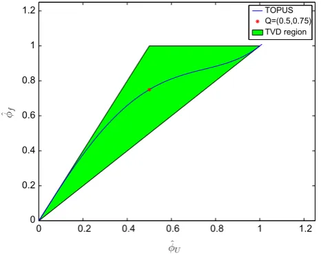
the superscript n will be omitted for simplicity. The CBC is a

condition for achieving computed boundedness if only three neigh-boring values are used to approximate the interface numerical

con-vected variables. According to Leonard [40,41], a bounded high

resolution second and/or third order accurate scheme (in general,

nonlinear) within the CBC region must pass through pointsO(0, 0),

Q(0.5, 0.75),P(1, 1) and with inclination of 0.75 atQ. Passing through

Qwill provide second order accuracy and passing throughQwith a

slope of 0.75 will give third order accuracy.

The TOPUS scheme is derived by assuming that the NV at the cell interfacef;/^f, are related to/^U by a fourth degree polynomial function for 0</^U<1, and a linear function (the FOU scheme) for ^

/U60 and /^UP1. The four conditions of Leonard presented

above, plus a free condition, are imposed to obtain

^ /f ¼

a

_/^4

Uþ ð2

a

þ1Þ/^3Uþ 5a410

_^

/2 Uþ aþ410

_^

/U;/^U2 ð0;1Þ;

^

/U; /^URð0;1Þ;

(

ð4Þ

where

a

is an adjustable constant in the interval [2,2]. If

a

= 0,

then TOPUS falls into the CBC region of Gaskell and Lau[24]and

corresponds to the SMARTER scheme of Choi and co-authors[19]

(see also Waterson and Deconinck[71]). By imposing an inclination

of 1 at pointP(i.e. a continuously differentiable function atP), one

obtains

a

= 2.Fig. 2depicts the TOPUS scheme for the case

a

= 2,

where one can see that it is entirely contained within the TVD re-gion of Harten[29]. Other values of

a

ensure that TOPUS falls within the CBC region. In practice, it is necessary to be careful. For

incom-pressible flows, it can be chosen from [2, 2] and boundedness will

be ensured; a good choice is

a

= 0 or

a

= 2. For compressible flows,

one must set

a

= 2 to guarantee the TVD criterion.

Letrfbe a local shock sensor satisfying Sweby’s monotonicity

preservation condition whenrftends to zero. Then the

correspond-ing flux limiter

w

=

w(

rf) for the TOPUS scheme when

a

= 2 is

de-duced as follows. The variable rf is the ratio of upstream to

downstream (consecutive) gradients

rf ¼

@/

@x f

@/

@x g

; ð5Þ

which, for uniform meshes, can be rewritten as

rf ¼

/U/R

/D/U

; ð6Þ

and, in terms of the NV, expressed as

rf ¼

^ /U

1/^U

: ð7Þ

Consider the general approximation (FOU scheme plus an anti-diffusive term) to the convected variable at thefface

^ /f ¼/^Uþ

1

2wðrfÞð1/^UÞ: ð8Þ

From Eq.(4), with

a

= 2, Eqs.(7) and (8), one determines

w(

rf) as

wðrfÞ ¼

ðjrfj þrfÞ½3rfþ1 ð1þ jrfjÞ

3 : ð9Þ

Fig. 3displays the TOPUS flux limiter(9)in therf

w(

rf) plane. It

can be seen that the TOPUS flux limiter is a smooth function ofrf

(>0) (see Zijlema[76]and Piperno et al.[49]), so there would appear to be a real possibility that it might perform better than other well recognized TVD schemes.

It is important to recognize that the TOPUS upwind scheme developed here, for calculating flux derivatives, is derived from 1D theory; and in multidimensional cases, it has to be applied (fol-lowing Zhang and Jackson[75]) to each of the coordinate directions separately.

2.2. Implementation issues

In this subsection, we show how TOPUS (and other upwinding schemes) may be incorporated into the discretized form of a num-ber of model equations. In addition, a brief discussion concerning the stability of the computations and the choice of the CFL param-eter is provided. In all calculations, for simplicity, first order

0 0.2 0.4 0.6 0.8 1 1.2

0 0.2 0.4 0.6 0.8 1

1.2 TOPUS

[image:3.595.43.278.555.740.2]

Q=(0.5,0.75) TVD region

Fig. 2.TOPUS witha= 2 on TVD region.

0 0.5 1 1.5 2 2.5 3 3.5 4

0 0.5 1 1.5 2 2.5

[image:3.595.315.542.557.737.2]

TOPUS P=(1,1) TVD region

explicit methods have been used for marching forward in time, ex-cept for the 1D inviscid Burgers equation, in which the 3th-order

accurate explicit TVD Runge–Kutta method [61] has been used,

and for the inviscid compressible flow over an airfoil, in which a second-order accurate, five-stage, explicit Runge–Kutta method

[32]has been employed.

2.2.1. The TOPUS scheme for 1D and 2D advection equation

The advection of a quantity/(x,t) by a convecting speed ais

modeled by the unsteady linear transport Eq.(1), where its exact

solution is given by/(x,t) =/0(xat), with/0(x) the initial

condi-tion. Eq. (1) is one of the simplest one-dimensional convection

models with a constant velocity contained within the initial data. Both varying the velocity fields and increasing the dimensions con-tribute to increased difficulties in modeling convection problems. But if a numerical scheme cannot solve the simple 1D case cor-rectly, then it will be of little use in more complex situations. The solution is, in the 1D case, approximated by the method given by Eq.(2), where the convected variable/, at thei1/2 andi+ 1/2

faces, is calculated using the upwind technology. Eq.(3)is then

employed to transform Eq.(4), with

a

= 2, giving

/i1=2¼

/Rþ ð/D/RÞ½2ð/^UÞ43ð/^UÞ3þ2/^U; /^U2 ð0;1Þ;

/U; /^URð0;1Þ;

(

ð10Þ

withD,UandRpreviously defined. The solution for the 2D case fol-lows similar lines.

The foregoing explicit numerical method has been imple-mented using an in-house computational fluid dynamics code, and its stability is governed by the CFL condition. In order to ensure stability, the time step is selected (automatically) in such a way

that the CFL parameter satisfies CFL61. Here, CFL denotes, in the

1D case, the maximum propagation speed in a control volume at

a given time level. In the 2D simulations, CFL¼maxjujdt

dxþ

maxj

v

jdt dx.

2.2.2. The TOPUS scheme for 1D convection–diffusion equations

We now consider a model of convection–diffusion, namely

@/ @tþ

e

@/ @x¼

m

@2/

@x2; ð11Þ

where the dependent variable/may, for example, be considered to

be a concentration in an incompressible fluid,

e

=

e

(/) and

m

is the

diffusion coefficient. When in Eq.(11)

e

= 1, the model corresponds

to a linear viscous flow model, with a boundary layer (see[22]). In

the case when

e

¼1

2/, Eq.(11)becomes the nonlinear viscous

Bur-gers’ equation[14]with

m

now interpreted as kinematic viscosity. It is well known that for large enough

m

> 0, smooth solutions are ob-tained, and the energy of the system dissipates smoothly. However, for

m

?0, discontinuities (shocks) can develop in the solution, even for prescribed smooth initial data. Burgers’ equation serves as a good model (combining nonlinear advection and linear diffusion) for understanding shock formation and turbulence. The numerical solution of this equation, in the linear case, is calculated in a man-ner similar to that used for solving the 1D advection equation in the previous subsection, with the diffusive term approximated by sec-ond order central differences. In the nonlinear case, the diffusive term is also approximated by the second order CD scheme, but the advection term (in the conservative form) is approximated by

e

ð/Þ@/ @x i ¼1 2 @/2 @x ! i ¼1 2

/iþ1=2/iþ1=2/i1=2/i1=2

2ðdx=2Þ

! ;

ð12Þ

with the advection velocities given by

/i1=2¼

1

2ð/iþ/i1Þ and /iþ1=2¼

1

2ð/iþ1þ/iÞ; ð13Þ

and the convected variable/at thei+ 1/2 andi1/2 calculed by

the TOPUS scheme (10). It is important to observe here that by

using the formula (13), for computing convection velocities, the

simple formula(12), which provides a simplified implementation

on the TOPUS, is rendered globally second-order accurate. However, in regions where the solution is sufficiently smooth, the order of convergence with the TOPUS scheme can be improved by implem-entating it in the context of flux function upwind reconstruction, associated with a high order time accuracy method and a suitable mesh refinement (similar to that appearing in Section 6, Eq. (84), of the Ref.[74]).

In the in-house numerical code equipped with the TOPUS

scheme, the stability condition for solving Eq.(11)and the choice

of the CFL parameter are made in a manner similar to the 1D advection equation.

2.2.3. The TOPUS scheme for 1D Euler equations

The one-dimensional flow of an inviscid and compressible gas

obeys the Euler equations (see, for example[32])

@U @tþ

@FðUÞ

@x ¼0; ð14Þ

where the conservative state vectorUand the convective flux

vec-torF(U) along thex-direction are defined by

U¼ ½

q

;

q

u;ET;

F¼ ½

q

u;

q

u2_{þp;uðEþpÞ}T

: (

ð15Þ

In the above vectors,xis distance,

q

density,uthex-component of velocity,ppressure, andEthe total energy per unit volume. The ra-tio of specific heats is set as

c

= 1.4 and, for a perfect gas, the system

is completed by the equation of state p= (

c

1)[E

q

u2_{/2]. Eq.}

(14)is numerically solved by using the explicit finite difference con-servative formula

Unþ1

i ¼U

n i þ

dt

dx

½Fi1=2Fiþ1=2

n

; ð16Þ

with the interface flux vector evaluated by using the method

pro-posed by Roe and Pike[51], namely: first the Roe average values

are computed (see Toro[62]); after that, fork= 1, 2, 3, the eigen-valuesekk and the eigenvectorsKeðkÞof the Jacobian matrixAb(both evaluated using averaging) are computed; next the wave strengths e

a

kare calculated; and then, with all of the aforementioned quanti-ties, the flux vectorsFi1/2and Fi+1/2(omitting for simplicity the

time index) are directly approximated by using flux limiters in

the framework of Sweby[60]. In particular, in a similar manner as

was done by Hubbard and Garcia-Navarro[31], we implement the

generic fluxFi+1/2as

Fiþ1=2¼FLOWiþ1=2þ

1 2

X3

k¼1

signð~_kkÞ~_{kkð1 jhkjÞw r}k f

ak

~ Ke

ðkÞ_j

iþ1=2; ð17Þ

where FLOWiþ1=2 is a monotone low-order accurate (building block)

numerical flux,hk¼~kkdt=dx, and

w(

) is the TOPUS flux limiter(9). The sensorrk

f is calculated by

rk f ¼ ~

a

upwind k ~

a

local k

; ð18Þ

where

a

~local

k ¼

a

~kjiþ1=2and

a

~ upwind

k is obtained at the upwind location

according to the velocity~_{kkat the facei+ 1/2. Finally, for the} build-ing blockFLOW

iþ1=2in Eq.(17)we use

FLOW iþ1=2¼

1

2ðFiþFiþ1Þ 1 2

X3

k¼1

~

The numerical method for solving 1D Euler equations is explicit, and its stability is governed by the CFL condition (see[10]). In this case, the time stepdtis assumed to satisfy

dt

dx

max k_iþ1 2

; kþ_iþ1 2

n o

61;

where k_iþ1

2 are the numerical acoustic waves associated with the

numerical flux function.

2.2.4. The TOPUS scheme for 2D Euler equations

The two-dimensional time-dependent Euler equations in con-servation form are

@U @t þ

@FðUÞ @x þ

@GðUÞ

@y ¼0; ð20Þ

where the conservative state vectorUand the convective flux

vec-torsF(U) andG(U) along thex- andy-directions, respectively, are defined by

U¼ ½

q

;

q

u;

q

v

;ET;

F¼ ½

q

u;

q

u2_þp;

_q

_u

_v

_;ðEþpÞuT

;

G¼ ½

q

v

;

q

u

v

;

q

v

2þp;ðEþpÞ

v

T;

E¼_ðcp1Þþ 1 2

q

ðu

2_þ

_v

2_Þ: 8

> > > > < > > > > :

ð21Þ

In Eqs.(20) and (21),

v

isy-velocity component; other constants and variables have been defined previously.

Two codes, implemented in the context of standard finite vol-ume methodology, were employed to solve the conservation law

systems(20) and (21): the software package CLAWPACK

(Conser-vation LAWs PACKage) of Leveque[42]and the code proposed by

Bigarella[11]. The TOPUS scheme was applied only in the specific

limiter routines of these codes. In particular, in the case of 2D aero-dynamic applications (two-dimensional limiters), the ideas of

Big-arella and Azevedo [12] were used to generalize the derivative

ratios, allowing the usage of any 1D limiter. In summary, the lim-iter

w(

rf) is an extension of the work of Barth and Jespersen[8]and is given by

wðrfÞ ¼ðj

rfj þrfÞ½3rf þ1 þ

LIM ð1þ jrfjÞ3þ

LIM

; ð22Þ

where

LIMis a control parameter designed to prevent singularities

(see[12]). The sensorrfcorresponds to the ratio of thef-th volume given by

rf ¼

numþ_{=den; if den>0;}

num_{=den; if den<0;}

1; if den¼0: 8

> < >

: ð23Þ

In the above equation,num±_{anddenare defined as (see[12,11])}

numþ_¼maxðq

i;qfÞ qi; num¼minðqi;qfÞ qi; den¼ ðqiÞfqi;

ð24Þ

withqia variable associated with the volumei,qfa variable associ-ated with the facefof the volume, and (qi)fa variable associated

with the volumeireconstructed at thefface.

2.2.5. The TOPUS scheme for 2D incompressible fluid flows

The conservation laws for time-dependent 2D incompressible fluid flow are the continuity and the momentum (Navier–Stokes) equations. In the Einstein index notation they are, respectively,

@ui

@xi

¼0; ð25Þ

@ui

@t þ

@uiuj

@xj ¼ @p

@xi þ1

Re

@ @xj

@ui

@xj

þ 1

Fr2gi; i¼1;2; ð26Þ

wheretis the time,xithe Cartesian coordinates,uithe

correspond-ing velocity components,pthe kinematic pressure,githe

compo-nents of the gravitational acceleration, and R= U0D/

m

and

Fr¼U0=

ffiffiffiffiffiffiffiffiffi Djgj p

, the Reynolds and Froude numbers, respectively. Here the usual Einstein summation convention is applied to

re-peated indices. The dependent variables in Eqs.(25) and (26)have

been nondimensionalized by a characteristic velocityU0, a length

scaleDand a reference kinematic viscosity

m

. To simulate the flow

problems modeled by Eqs.(25) and (26), the primitive variable Mar-ker-And-Cell (MAC, Los Alamos) method was used: this is a special

case of the projection method of Chorin[20]described by Harlow

and Welch[30](see also McKee et al.[45]). This finite difference

method, defined on a staggered grid system, has been incorporated

into the 2D version of the Freeflow code[16]. The MAC method uses

massless marker particles, which are employed to indicate the fluid configuration showing which regions are occupied by fluid and which are empty. At each time step, the marker particles are moved to new positions using local fluid velocities.

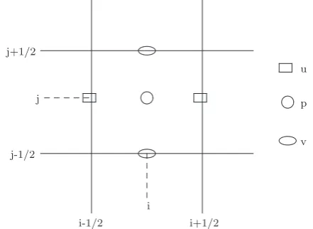
For the spatial advection terms of the Navier–Stokes Eq.(26),

the application of the TOPUS scheme is as follows. For the stag-gered grid used in this paper, afface for discretization can assume one of the following faces of the control volume depicted inFig. 4:

iþ1

2;j

or i;jþ1

2

:

The convected variable/, calculated by the TOPUS scheme, can be

one of the velocity componentsuor

v

. For conciseness, only the

dis-cretization of the nonlinear advection terms in theu-component of

the Navier–Stokes equations will be presented. The discretization of the other nonlinear terms are similar. In the position iþ1

2;j

of the

2D computational mesh (seeFig. 4), this term can be approximated

by the following conservative scheme:

@ðuuÞ @x þ

@ðu

v

Þ @y

jiþ1 2;j

uiþ1;juiþ1;jui;jui;j

dx

þ

v

iþ1

2;jþ12uiþ12;jþ12

v

iþ12;j12uiþ12;j12 dy

;

where the advection velocitiesuiþ1;j;ui;j;

v

iþ1

2;jþ12and

v

iþ12;j12 are

ob-tained by averaging, in a similar manner as in Eq.(13)for Burgers’ equation, and the convected velocities follow similar procedures to that in Eq.(12). The following criterion was used for selecting an appropriate time step

dt¼minfFACT1dtCFL;FACT2dtVISCg;

where 0 <FACT161 and 0 <FACT261 are constants chosen to

[image:5.595.317.538.569.730.2]

en-sure that the calculations are stable with

Fig. 4.Cell-variable locations for 2D calculation, showing the faces whereuandv

dtCFL¼max dx juj;

dy j

v

j

and dtVISC¼

Re

2

d2xd 2 y

d2xþd 2 y

:

2.2.6. Popular upwinding schemes

In this subsection, we list the schemes that are to be compared

with TOPUS. We also detail flux limiter functions.Non-normalized

variable schemes:

SMART[24]:

/f¼

/U if /^UR½0;1;

10/U9/R if 06/^U<3=74;

1

8ð3/Dþ6/U/RÞ if 3=746/^U<5=6;

/D if 5=66/^U61;

8 > > > > > < > > > > > :

VONOS[65]:

/f¼

/U if/^UR½0;1;

10/U9/R if 06/^U<3=74;

3

8/Dþ34/U18/R if 3=746/^U<1=2;

1:5/U0:5/R if 1=26/^U<2=3;

/D if 2=36/^U61;

8 > > > > > > > > > < > > > > > > > > > :

WACEB[57]:

/f¼

/U if/^UR½0;1;

2/U/R if 06/^U<3=10;

3

4/U38/D18/R if 3=106/^U<5=6;

/D if 5=66/^U61;

8 > > > > > < > > > > > :

0 0.2 0.4 0.6 0.8 1 1.2

100 100.2 100.4 100.6 100.8 101

Exact ADBQUICKEST

0 0.2 0.4 0.6 0.8 1 1.2

100 100.2 100.4 100.6 100.8 101

Exact SMART

0 0.2 0.4 0.6 0.8 1 1.2

100 100.2 100.4 100.6 100.8 101

Exact WACEB

0 0.2 0.4 0.6 0.8 1 1.2

100 100.2 100.4 100.6 100.8 101

Exact VONOS

0 0.2 0.4 0.6 0.8 1 1.2

100 100.2 100.4 100.6 100.8 101

Exact van Albada

0 0.2 0.4 0.6 0.8 1 1.2

100 100.2 100.4 100.6 100.8 101

[image:6.595.119.486.69.469.2]

Exact TOPUS

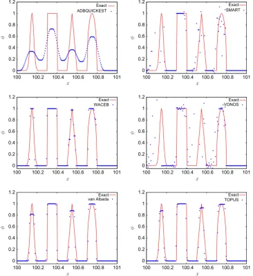
[image:6.595.314.520.514.748.2]

Fig. 5.Test case 1: numerical (blue symbol) and exact (red line) of the unsteady linear advection equation. (For interpretation of the references to colour in this figure legend, the reader is referred to the web version of this article.)

Table 1

Computing time per mesh point per iteration and normalized costs by the unit cost of the WACEB scheme (cheapest).

Scheme Unit cost (ls) Normalized costs

ADBQUICKEST 0.35 1.13

SMART 2.13 6.87

WACEB 0.31 1.00

VONOS 1.45 4.68

van Albada 0.33 1.06

Superbee[7]:

/f ¼

/U if /^UR½0;1;

2/U/R if 06/^U<1=3; 1

2ð/Dþ/UÞ if 1=36/^U<1=2; 3

2/U12/R if 1=26/^U<2=3;

/D if 2=36/^U61;

8 > > > > > > > < > > > > > > > :

CUBISTA[5]:

/f ¼

/U if /^UR½0;1;

7

4/U34/R if 06/^U<3=8; 3

8/D34/U18/R if 3=86/^U<3=4; 3

4/Dþ14/U if 3=46/^U61;

8 > > > > > < > > > > > :

ADBQUICKEST[23]:

/f ¼

/U if/^UR½0;1;

ð2hÞ/U ð1hÞ/R if 06/^U<a;

aD

/Dþ

aU

/U

aR

/RÞ ifa6/^U6b; ð1hÞ/Dþh/U ifb</^U<1;

8 > > > > < > > > > :

with

a

D¼1₆ð23hþh2Þ;

a

U¼1₆ð5þ3h2h2Þ;

a

R¼1₆ð1h2Þ;

a¼ 23hþh

2

79hþ2h2; b¼

4þ3hþh2 5þ3hþ2h2:

Flux limiter functions:

Minmod[28]:

w(

rf) = minmod (1,rf);

Superbee[7]:

w(

rf) = max (0, min (1, 2rf), min (2,rf));

monotonized centered (MC)[67]:

w(

rf) = max (0, min ((1 +rf)/ 2, 2, 2rf));

van Leer[66]:wðrfÞ ¼

rfþ jrfj 1þ jrfj ;

van Albada[64]:wðrfÞ ¼

r2 f þrf 1þr2 f

;

ADBQUICKEST [23]:

wðrfÞ ¼max 0;min 2rf;

2þh2_3hþð1h2_Þr f

33h ;2

n o

n o

:

3. Numerical experiments

[image:7.595.33.555.85.336.2]

In order to demonstrate the behavior, validity, flexibility, robustness and practicality of the TOPUS scheme, we have per-formed numerous simulations based on benchmark test cases, including 2D compressible/incompressible flows. Comparisons are made both with exact solutions and with well-recognized

Table 2

Errors and computed convergence rates for 2D advection equation, with CFL = 0.5 at timet= 2. Here, ADB refers to ADBQUICKEST.

Scheme Mesh L1-error Convergence rate L2-error Convergence rate

ADB 1616 7.40e3 – 3.00e2 –

3232 1.81e3 2.0 1.09e2 1.5

6464 4.74e4 1.9 4.14e3 1.4

128128 1.20e4 2.0 1.50e3 1.5

256256 3.03e5 2.0 5.37e4 1.5

Superbee 1616 8.94e3 – 3.63e2 –

3232 1.87e3 2.3 1.15e2 1.7

6464 4.60e4 2.0 4.05e3 1.5

128128 1.19e4 2.0 1.49e3 1.4

256256 3.02e5 2.0 5.35e4 1.5

van Leer 1616 6.97e3 – 2.81e2 –

3232 1.82e3 1.9 1.09e2 1.4

6464 4.74e4 1.9 4.14e3 1.4

128128 1.20e4 2.0 1.50e3 1.5

256256 3.03e5 2.0 5.37e4 1.5

van Albada 1616 8.85e3 – 3.61e2 –

3232 4.47e3 1.0 2.67e2 0.4

6464 6.08e4 2.9 5.29e3 2.3

128128 1.46e4 2.1 1.82e3 1.5

256256 3.40e5 2.1 6.02e4 1.6

TOPUS 1616 1.01e2 – 4.09e2 –

3232 3.39e3 1.6 2.02e2 1.0

6464 5.63e4 2.6 4.91e3 2.0

128128 1.34e4 2.1 1.67e3 1.6

[image:7.595.32.555.644.754.2]

256256 3.20e5 2.1 5.66e4 1.6

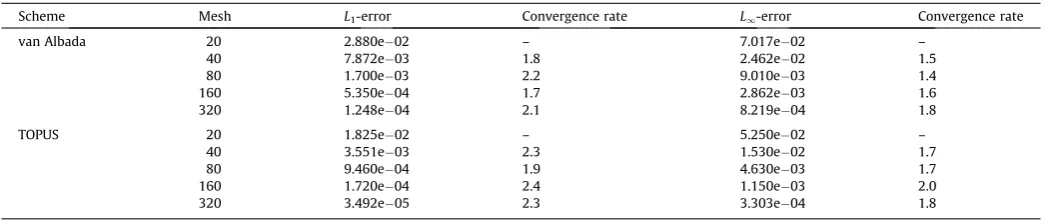
Table 3

Errors and computed convergence rates for 1D inviscid Burgers’ equation, withu0(x) = 1 + 0.5sin(px),1 <x< 1 at timet= 0.12.

Scheme Mesh L1-error Convergence rate L1-error Convergence rate

van Albada 20 2.880e02 – 7.017e02 –

40 7.872e03 1.8 2.462e02 1.5

80 1.700e03 2.2 9.010e03 1.4

160 5.350e04 1.7 2.862e03 1.6

320 1.248e04 2.1 8.219e04 1.8

TOPUS 20 1.825e02 – 5.250e02 –

40 3.551e03 2.3 1.530e02 1.7

80 9.460e04 1.9 4.630e03 1.7

160 1.720e04 2.4 1.150e03 2.0

high-resolution bounded schemes. The formal order of accuracy of the schemes is 2, except for TOPUS, ADBQUICKEST, WACEB, SMART and 3rd-WENO schemes. For the second order spatial derivatives and pressure terms, second order CD was employed. In all numer-ical tests presented in this article, the TOPUS scheme is used with

a

= 2. For compressible flow calculations, the parameter

LIM

(appearing in Eq.(22)) is set as 107_{. All simulations have been}

per-formed on a Sony VAIO VGN-CS325J laptop with a Intel Core 2 Duo T6500/ 2.1 GHz (Dual-Core) processor and 4 Gbytes RAM running Linux 2.6.30-bpo.2-amd64.

3.1. 1D scalar advection problem

The first test case consists of the advection of a quantity/(x,t)

with a convecting speed a= 1 modeled by the unsteady linear

advection Eq.(1). The physical relevance of this problem is that

it models entropy waves in gas dynamics. In this test case, Eq.

(1),x2[0, 101], is solved in conjunction with the following combi-nation of smooth and sharp distributions as initial condition:

1/0ðxÞ ¼

e

log50 x0:15

0:05

2

; x2 ½0;0:2Þ;

1; x2 ð0:3;0:4Þ;

20x10; x2 ð0:5;0:55Þ;

1220x; x2 ½0:55;0:66Þ; ffiffiffiffiffiffiffiffiffiffiffiffiffiffiffiffiffiffiffiffiffiffiffiffiffiffi

1 x0:75 0:05

2

q

; x2 ð0:7;0:8;

0; otherwise:

8 > > > > > > > > > > > > > < > > > > > > > > > > > > > :

ð27Þ

In the foregoing numerical simulations, a mesh size of N= 2200

computational cells was adopted with time spacing dt= 0.0025

and the final simulation timet= 100.0.Fig. 5depicts the exact solu-tion and the numerical results obtained with ADBQUICKEST, SMART, WACEB, VONOS, van Albada and TOPUS schemes. It can be seen from this figure that, for long simulation times, WACEB, van Albada and TOPUS schemes perform reasonably well, but exhi-bit the peak ‘‘clipping’’ problem.

The unit costs (computation time per mesh point per iteration) and the unit normalized costs for the various choice of limiters are

provided inTable 1. The cost for the TOPUS scheme is smaller than

the corresponding costs for SMART, VONOS, ADBQUICKEST and van Albada schemes, but higher than that for WACEB scheme. The com-putations were then carried out on a sequence of meshes and sim-ilar patterns were observed.

3.2. 2D scalar advection problem

We choose the 2D scalar convection equation, on the unit square, to check the numerical order of accuracy of the TOPUS scheme, with the advection velocitiesu=

v

= 1, the initial condition

/0ðx;yÞ ¼sinð2

p

xÞsinð2

p

yÞ ð28Þ

and with periodic boundary conditions. The exact solution is given by (see[78])

0 0.1 0.2 0.3 0.4 0.5 0.6

-1.5 -1 -0.5 0 0.5 1

Exact ADBQUICKEST

0 0.1 0.2 0.3 0.4 0.5 0.6

-1.5 -1 -0.5 0 0.5 1

Exact SMART

0 0.1 0.2 0.3 0.4 0.5 0.6

-1.5 -1 -0.5 0 0.5 1

Exact TOPUS

0 0.1 0.2 0.3 0.4 0.5 0.6

-1.5 -1 -0.5 0 0.5 1

[image:8.595.121.483.67.332.2]

Exact VONOS

Fig. 6.Solution of the Riemann problem for the inviscid Burgers’ equation using the initial condition(29).

0 0,5 1 1,5 2

[image:8.595.51.287.366.560.2]

0,99 0,995 1

/ðx;y;tÞ ¼sinð2

p

ðxtÞÞsinð2

p

ðytÞÞ:

Table 2gives theL1andL2errors and the corresponding orders of

convergence for the ADBQUICKEST, Superbee, TOPUS, van Albada

and van Leer schemes with CFL = 0.5 at final timet= 2. Practically,

the same order of convergence is observed for all schemes. The numerical results are omitted here to save space.

3.3. 1D Burgers’ equation

Here simulations are performed for the classic 1D Burgers’

equation, namely Eq.(11)with/=uand

¼1

2u. Both the inviscid

(

m

= 0.0) and viscous (

m

= 0.05) cases are considered. Firstly, we solve the inviscid case with a smooth initial distribution to study the convergence. Next, we employ a specific initial distribution to assess the shock capturing capabilities of the schemes. We ad-dress, in the following, the nonlinear stability of the TOPUS scheme. Finally, by resolving the viscous case, we check the impact of the flux function upwind reconstruction on the TOPUS’s conver-gence rate.

The accuracy of the spatial discretization is checked by solving

Eq. (11), x2[1, 1], with the smooth initial distribution

u(x,0) = 1 + 0.5sin(

p

x). The third order accurate TVD Runge–Kutta

method presented in Tang and Warnecke[61]was used for

evolu-tion in time. The accuracy for all the popular upwinding schemes,

given in Section 2.2.6, and that for Shu and Osher’s third-order

WENO are shown to be O(h5/2_{) in both the discrete L}

1 and L1 norms. The FOU scheme using a mesh size of 800 cells has been

used for determining errors. In particular, Table 3 summarizes

the errors and convergence rates observed foruat time t= 0.12

for the TOPUS and van Albada schemes. One can see that, for this nonlinear test case, convergence rates in excess of second order is obtained several times with the TOPUS scheme. One possible reason for these rates may be the rapid dampening of oscillations

in the computed variableuas the mesh increases.

[image:9.595.31.555.96.187.2]

The shock capturing property of the TOPUS scheme is studied by solving(11)with the initial distribution

Table 4

Comparison of the errors and convergence orders for 1D viscous Burgers’ equation at time 0.25, fordt= 0.001, using the simplified and flux function upwind reconstruction modes. Measured errors as function of the mesh size andRe= 20.

Mode Mesh L1-error Order L2-error Order L1-error Order

Simplified 25 9.374e4 – 1.696e3 – 4.035e3 –

50 3.045e4 1.6 5.012e4 1.8 1.089e3 1.9

100 9.111e5 1.7 1.400e4 1.8 2.887e4 1.9

200 2.472e5 1.8 3.700e5 1.9 7.420e5 2.0

Flux function 25 2.772e3 – 3.574e3 – 5.729e3 –

50 5.595e4 2.3 7.360e4 2.3 1.228e3 2.2

100 9.544e5 2.6 1.222e4 2.6 2.238e4 2.5

200 1.397e5 2.8 1.797e5 2.8 3.374e5 2.7

20 40 60 80 100

−15 −10 −5 0

Iterations

Log (Residual)

[image:9.595.38.280.111.392.2]

Simplified Flux function

[image:9.595.35.552.548.754.2]

Fig. 8.Convergence history obtained with the TOPUS scheme, implemented in the context of simplified and flux function upwind reconstruction modes, for the 1D viscous Burgers’ equation at Re = 20.

Table 5

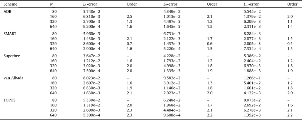
Comparison of the errors for 1D scalar convection–diffusion equation, at different times, fordt= 0.01/N. Measured errors as function of the mesh size andRe= 100. ADB refers to ADBQUICKEST.

Scheme N L1-error Order L2-error Order L1-error Order

ADB 80 3.748e2 – 4.349e2 – 5.545e2 –

160 6.810e3 2.5 1.013e2 2.1 1.379e2 2.0

320 2.700e3 1.3 4.497e3 1.2 6.299e3 1.1

640 9.200e4 1.6 1.645e3 1.5 2.311e3 1.4

SMART 80 5.960e3 – 6.731e3 – 8.284e3 –

160 1.430e3 2.1 2.122e3 1.7 2.877e3 1.5

320 8.600e4 0.7 1.437e3 0.6 2.005e3 0.5

640 2.900e4 1.6 5.220e4 1.5 7.334e4 1.5

Superbee 80 3.647e2 – 4.228e2 – 5.386e2 –

160 1.212e2 1.6 1.793e2 1.2 2.404e2 1.2

320 3.020e3 2.0 4.998e3 1.8 6.970e3 1.8

640 7.500e4 2.0 1.335e3 1.9 1.888e3 1.9

van Albada 80 8.023e2 – 9.582e2 – 1.266e1 –

160 2.607e2 1.6 3.912e2 1.3 5.401e2 1.2

320 6.830e3 1.9 1.140e2 1.8 1.601e2 1.8

640 1.630e3 2.1 2.923e3 2.0 4.122e3 2.0

TOPUS 80 5.330e2 – 6.248e2 – 8.073e2 –

160 1.319e2 2.0 1.968e2 1.7 2.692e2 1.6

320 2.690e3 2.3 4.484e3 2.1 6.278e3 2.1

uðx;0Þ ¼

0:0; ifx6₁;

0:5; if 1<x<0;

0:0; ifxP0: 8

> < >

: ð29Þ

The exact solution is the rarefaction wave given by Ahmed (see[3]):

uðx;tÞ ¼

0:0; ifx61;

xþ1

t ; if 1<x6 t 21;

0:5; if t

21<x< t 4;

0:0; ifxPt 4: 8

> > > < > > > :

This problem consists of a jump from zero to one atx=1/3 which

creates an expansion fan, while the jump from one to zero atx= 1/3

produces a shock wave. The purpose of this test is to check whether

1 1.5 2 2.5 3 3.5 4 4.5 5

1 1.5 2 2.5 3

Reference ADBQUICKEST, N = 200 ADBQUICKEST, N = 300

1 1.5 2 2.5 3 3.5 4 4.5 5

1 1.5 2 2.5 3

Reference Lax-Wendroff, N = 200 Lax-Wendroff, N = 300

1 1.5 2 2.5 3 3.5 4 4.5 5

1 1.5 2 2.5 3

Reference MINMOD, N = 200 MINMOD, N = 300

1 1.5 2 2.5 3 3.5 4 4.5 5

1 1.5 2 2.5 3

Reference Superbee, N = 200 Superbee, N = 300

1 1.5 2 2.5 3 3.5 4 4.5 5

1 1.5 2 2.5 3

Reference van Leer, N = 200 van Leer, N = 300

1 1.5 2 2.5 3 3.5 4 4.5 5

1 1.5 2 2.5 3

[image:10.595.124.483.67.465.2]

Reference TOPUS, N = 200 TOPUS, N = 300

[image:10.595.83.259.504.602.2]

Fig. 9.Density distribution for the Shu–Osher shock tube problem using ADBQUICKEST, Lax-Wendroff, Minmod, Superbee, van Leer and TOPUS schemes.

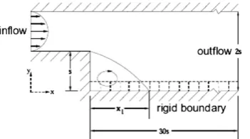
Fig. 10.Geometry of the backward facing step problem, showing a set of

computational cells adjacent to the wall.

200 400 600 800

2 4 6 8 10 12 14 16

Armaly et al. (Num.) Armaly et al. (Exp.) Ku et al. Jiang et al. Williams and Baker 2D Williams and Baker 3D TOPUS

ADBQUICKEST

[image:10.595.325.550.507.681.2]

the TOPUS scheme needs an additional smooth transition function

(or not) to avoid entropy violation. A mesh size ofN= 200

compu-tational cells, final time t= 2, x2[1.5, 1] and dt= 0.01125 were used in the simulation. The numerical results obtained with ADB-QUICKEST, SMART, TOPUS, and VONOS schemes and the exact solu-tion are presented inFig. 6. Once again, it is seen that in comparison with the other methods TOPUS gives satisfactory results, capturing quite well the expansion fan and the shock wave without the need for adding an entropy correction formula.

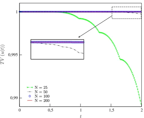
Before concluding this section, we address the issue of nonlin-ear stability for the TOPUS scheme by checking the numerical time dependent total variation (TV) on progressively refined mesh sizes

using the nonlinear problem(11)subject to the initial condition

(29). Fig. 7shows the TV calculated forN= 25, 50, 100 and 200 computational cells. It can be seen that as time progresses the TV decreases or remains constant indicating that there is no loss of TV at local extrema.

Finally, the viscous Burgers’ equation is solved in order to show that, for smooth solutions, the accuracy of the TOPUS scheme can

be improved by implementating it in the flux function upwind reconstruction mode (similar to that appearing in Section 6, Eq.

(84), in Ref.[74]). The boundary conditions are chosen equal to

be u(0,t) = tanh (Re/4) and u(1,t) =u(0,t), with Re= 1/

m

= 20. The initial condition is taken from the exact steady state solution

in[22]. The observed order of accuracy with the TOPUS scheme,

computed with both simplified and flux function reconstruction

implementation modes, is depicted in Table 4. One can clearly

see that, with the use of the flux function implementation, the TO-PUS’s convergence rate is improved. Also shown inFig. 8is the con-vergence history obtained with the TOPUS scheme, on a mesh size of 200 computational cells, using both simplified and flux function implementations. The explicit Euler method was used for the time March in this test case. The TOPUS scheme converges rapidly, at about thirteen orders of magnitude reduction in the residual. Therefore, in this paper, for all nonlinear problems involving con-vection–diffusion effects, we will use, for simplicity, the simplified

implementation version of the TOPUS scheme given by Eqs.(12)

and (13).

3.4. 1D scalar convection–diffusion equation

Having solved linear and nonlinear equations with different ini-tial data, we now consider the most popular 1D scalar convection– diffusion model (11) with 0 <x< 1 and

e

= 1 (the so-called 1D boundary layer problem). The initial and boundary conditions are

u(x, 0) = 0 and u(0,t) = 0;u(1,t) = 1, tP0, respectively. The exact steady state solution of this problem on theicell ((idx)(06i6N)) is

gi-ven by (see[22])ui= (1exp (iRed))/(1exp (Re)), whereRed=Re

dxdenotes the cell Reynolds number. The solution is obtained on a

series of refined grids (fromN= 80 up to N= 640 computational

cells). A numerical convergence study is performed from

calcula-tions on several grids.Table 5depicts the computed convergence

rate when the ADBQUICKEST, SMART, Superbee, van Albada and

TOPUS schemes are used for this problem forRe= 100. It can be

seen from this table that theL1,L2 andL1 errors for the TOPUS scheme decrease with increasing grid points (mesh refinement), indicating convergence. In addition, the TOPUS scheme shows

-0.3 -0.25 -0.2 -0.15 -0.1 -0.05 0 0.05 0.1 0.15 0.2

1 1.2 1.4 1.6 1.8 2 2.2 2.4

TOPUS mesh 200 x 10

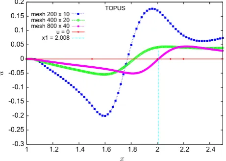
[image:11.595.44.275.70.234.2]

mesh 400 x 20 mesh 800 x 40 u = 0 x1 = 2.008

Fig. 12.Convergence test for the numerical solution foruvelocity of the flow over a backward facing step at Reynolds numberRe= 400.

[image:11.595.70.517.492.732.2]

improved numerical orders of accuracy compared with the global accuracy of the other schemes. The accuracy analysis performed here seems to indicate the dominant error is, in fact, the second-order truncation error arising from the discretization of the diffu-sive term. In particular, the numerical diffusion introduced by TO-PUS is significantly smaller than the physical diffusion coefficient

m

.

3.5. 1D Shu–Osher’s shock tube problem

In order to verify that the TOPUS scheme is effective in prevent-ing oscillations in unsteady flows, the 1D inviscid Euler Eq.(14)of gas dynamics was solved. The problem that was chosen is the Shu–Osher’s shock tube[56](see also[74]), that describes a shock interacting with smooth density fluctuations. This case provides a good test for examining the performance of the high order upwind schemes, because it possesses both strong discontinuous and

smooth structures. Here, Eq. (14) is considered in the interval

[1, 3] with the initial condition

ð

q

;

t

;pÞT¼ ð3:86;2:63;10:33Þ T

; if x2 ½1;0:8Þ; ð1þ0:2 sinð5xÞ;0;1ÞT; if x2 ½0:8;3: (

ð30Þ

In this case, two meshes (N= 200 withdx= 0.02 andN= 300 with

dx= 0.0133), time spacingdt= 0.6dxand final timet= 1.0 are used. The numerical results for density using ADBQUICKEST, Lax-Wendroff, Minmod, Superbee, van Leer and TOPUS schemes, and

the reference solution (FOU scheme withN= 2000) are presented

in Fig. 9. One can observe that TOPUS provides reasonable

resolution.

3.6. 2D incompressible flow over a backward facing step

The flow over a backward facing step, comprehensively studied over the years and extensively used to analyze the quality of schemes, is computed here for laminar flow. The relevant conser-vation laws for 2D time-dependent incompressible fluid flow are

the continuity(25)and the momentum (Navier–Stokes)(26)

equa-tions. The geometry of the problem is illustrated in Fig. 10. This

problem is challenging computationally as it involves flow separa-tion and recirculasepara-tion. The size and locasepara-tion of the separasepara-tion zone is very sensitive to the pressure gradient, thereby providing a good flow validation test case. Furthermore, there is extensive numerical and experimental data available in the literature. With a fully developed Poiseuille parabolic velocity profile prescribed at the

0 0,2 0,4 0,6 0,8 1

0 0,5 1 1,5 2

Reference TOPUS van Albada

0 0,2 0,4 0,6 0,8 1

-2 -1 0 1 2

[image:12.595.122.489.69.196.2]

Reference TOPUS van Albada

Fig. 14.Results for complex interacting flow structure problem along the diagonal (x=y) line. On the left, density distribution and on the right pressure distribution.

[image:12.595.67.531.470.735.2]

inlet section, we simulated numerically this fluid flow problem for a wide range of Reynolds numbers. These were based on the

max-imum velocityU0=Umax= 1 m/s at the entrance section and the

height of the steps(s=D= 0.1 m). The dimension of the

computa-tional domain is 4.0 m 0.2 m and the total time of simulation is

100 seconds. A mesh size of 80040 computational cells has been

used in the simulations.

Fig. 11 graphically displays the evolution of reattachment

lengthsx1, normalized by the step heights. With Reynolds

num-bers from 100 up to 800, we have the following data: 2D numerical results of Armaly et al.[6]and Willians and Baker[72]; 3D numer-ical results of Willians and Baker[72], Ku et al.[36], Jiang et al.[34]

and the experimental data of Armaly et al.[6]. We also have

calcu-lations using TOPUS and ADBQUICKEST schemes (no significant improvement was observed in the results obtained using the other

schemes). The numerical results using ADBQUICKEST, for

0 <Re< 400, show good agreement with the 2D results of Willians

and Baker[72]; they would appear, however, to diverge from the

data of Armaly et al.[6]and the 3D calculations. ForReP 400,

the numerical results of both TOPUS and ADBQUICKEST give poor agreement with 3D data; this may be explained by 3D effects and, possibly, the turbulence transition in this high Reynolds

num-ber problem, as postulated by Ghia et al. [26]. This figure also

shows a close-up, where it can be seen that the results obtained with the TOPUS scheme are marginally better than those obtained using the ADBQUICKEST scheme.

In addition, a convergence test of the numerical solution for

(streamwise) velocity componentu was performed with a

Rey-nolds number of 400 on three uniform meshes consisting of

20010, 40020 and 80040 cells. This is illustrated in

Fig. 12, which shows how the reattachment length x1 was

esti-mated (i.e. the change in the sign of theuvelocity profile adjacent

to the lower bounding wall (seeFig. 10)).

3.7. 2D compressible Euler equations

In this section, the TOPUS scheme is used to solve the 2D

com-pressible Euler equations in conservative form(20)for steady and

unsteady flows. The specific problems considered here are: (i) the shock–shock interaction problem originally defined by

Schulz-Rinne et al. [53] (see also [15]) in the square domain

[0, 1][0, 1]; and (ii) the steady transonic flow around the NACA

0012 airfoil withM1= 0.85 and

a

= 1°.

Computations for the shock–shock interaction problem were

performed by using the CLAWPACK software[42], implemented

with TOPUS, van Albada and MC limiter of van Leer[67](see also

[42]p. 115, or[27]). In the version of the CLAWPACK code that

we have used, the Godunov’s first-order explicit time marching method with second-order spatial corrections is implemented, where the flux functions are calculated by solving local Riemann problems; this allows the easy introduction of limiter functions to give high-resolution results. The solution of the problem using

the MC limiter, on a mesh size of 20002000 computational cells,

was selected as a reference solution, since this limiter has been one of the more widely used in engineering applications (see, for

in-stance [18,38] or [27]). This problem, a useful test to measure

the smallness of the inherent numerical viscosity of the scheme, Iterations

Log (Residual)

0 20000 40000 -6

-4 -2 0 2

[image:13.595.310.543.66.533.2]

van Albada T OPUS

Fig. 16.Convergence histories with van Albada and TOPUS schemes for a NACA 0012 airfoil atM1= 0.85 anda= 1°.

X/C

Cp

0 0.25 0.5 0.75 1

-1

-0.5

0

0.5

1

van Albada TOPUS

X/C

Cp

0.7 0.8 0.9

-1

-0.5

0

van Albada TOPUS

Fig. 17.Comparison between numerical results obtained with TOPUS and van

Albada limiters for the pressure coefficient distributions for a NACA 0012 airfoil at

[image:13.595.46.270.67.271.2]

arises frequently as a model for simulating thin shear layers or

sharp interfaces between inviscid fluids[52]. The solutions were

marched in time until time t= 0.8 by using a mesh size of

200200 computational cells and at CFL number of 0.8. Fig. 13

shows density contour lines computed with TOPUS and van Albada limiters. One can observe that TOPUS provides qualitatively the same resolution as van Albada except at the top right region, where the TOPUS limiter captures the vortical structures a little better. However, when the density and pressure profiles are plotted along the diagonal (x=yline), as shown inFig. 14, significant differences between the TOPUS and the van Albada solutions can clearly be ob-served, indicating that TOPUS has behaved somewhat better than the van Albada limiter. In addition, to show that the TOPUS scheme is capable of capturing the complex interacting structures in the

flow (i.e., vortex sheets), we repeat the numerical experiment

shown inFig. 13using a mesh size of 15001500 computational

cells. The density contour lines are depicted inFig. 15, from which it can be seen that the TOPUS scheme provides a substantial improvement at the contact surface, where instabilities manifest themselves. So, it would appear that the TOPUS limiter introduces less numerical viscosity than van Albada.

We now focus on the specific AGARD test case (see[2]) of the

steady inviscid compressible flow over a NACA 0012 airfoil at

free-stream Mach numberM1= 0.85 and angle-of-attack

a

= 1 deg. The

objective of this test is to investigate whether the TOPUS scheme could resolve flows possessing strong shocks as well as the van Albada limiter, a widely used upwinding scheme for compressible flow computations. This classical case is computed using a mesh size of 251 points over the airfoil surface, 151 points in radial direc-tion and the farfield boundary is set at 70 chords of radius. The solution is obtained using single-precision operations. The CFL number is set as a constant value of 0.7 and the maximum density

residual for accepting convergence is chosen to be 107_{. Time}

March to steady state uses the 5-stage, 2th-order accurate, explicit

Runge–Kutta method presented in Ref.[32]. InFig. 16, the

conver-gence curves obtained with the van Albada and TOPUS schemes are presented, showing that both schemes converge, at about the same rate, with eight orders of magnitude reduction in the residual.

The pressure coefficient distributions, Cp, on the upper and

lower surfaces of the airfoil obtained with TOPUS and van Albada limiters are plotted inFig. 17. The overall views of theCp

distri-butions are shown in Fig. 17a and detailed views of the upper

and lower surface shock waves are shown inFig. 17b. From these

figures, it is seen that both TOPUS and van Albada limiters pro-vide similar results, showing that the strength of the shock is in

good agreement with the ones given in [2]. The results are also

indicating that the shocks can be captured by the TOPUS scheme with 1–2 mesh points, whereas 3–4 points in the shock transition are observed when the van Albada limiter is used. The data in

Fig. 17b also indicate that TOPUS is slightly less dissipative than the van Albada limiter at the shock. Away from the shock waves, both TOPUS and van Albada schemes produce almost identical results.

Further investigation of these results can be achieved by inspecting the entropy generated by the numerical solutions. Hence,Fig. 18presents the entropy generated at the airfoil surface by the two schemes for the same flight condition. Moreover, the

entropy fields are shown inFig. 19a and b for van Albada and

TO-PUS schemes, respectively. The clear conclusion from these figures is that the entropy generated by the two schemes is quite

compa-rable. InFig. 18, one can see that TOPUS creates slightly more

en-tropy at the airfoil surface than the van Albada limiter. Again, these results emphasize that TOPUS has essentially the same shock cap-turing characteristics as the widely used van Albada limiter for such inviscid transonic applications.

Finally, drag and lift coefficients (CdandCl) are summarized in

Table 6. In this particular case, besides the comparison between TOPUS and van Albada schemes, we have included results for the

present test case obtained by Amaladas and Kamath[1], Jameson

and Martinelli[33]and by Pulliam and Barton[50]. The table also

includes the range of values for lift and drag coefficients reported

in [2]. Such data provide for a more quantitative comparison of

the presently proposed scheme. One can see inTable 6that the

present results for lift and drag coefficients are between those pro-vided by the van Albada limiter and those propro-vided by the centered schemes. Again, the current results are very close to those provided by the van Albada limiter, except that we obtain a slightly higher value of lift coefficient, which is probably a consequence of the less dissipative behavior at the shock, as previously discussed, and also a somewhat higher drag coefficient. We believe that the higher drag coefficient is associated with the fact that TOPUS is generating slightly more entropy at the airfoil surface than the van Albada

limiter, as indicated inFig. 18. Hence, TOPUS produces more

spuri-ous drag than the van Albada limiter, explaining the higherCd

val-ues. However, one should notice that, clearly, such additional spurious drag is quite lower than what is generated by the other

schemes compared in Table 6. Furthermore, the current results

for both lift and drag coefficients are well within the ranges re-ported in[2].

4. Closing remarks

A high degree polynomial upwind-based finite difference scheme (TOPUS) has been introduced for the numerical solution of convection-dominated transport problems. This new scheme was derived from the application of the TVD/CBC stability criteria

combined with the four conditions of Leonard[41]. TOPUS is

pre-sented in both the normalized variables of Leonard and also as a flux limiting technique, and has been shown to possess three important features: simplicity, robustness and generality of

appli-cation. By setting the free parameter

a

equal to 2, the scheme is

then guaranteed to be oscillation-free; and, with this value of

a

,

the performance of the scheme was evaluated by solving a variety of test problems. These included the 1D/2D advection of scalars, the 1D Riemann problem for Euler’s/Burgers’ equation, the 2D Rie-mann problem for Euler’s equation, the 2D incompressible Navier– X/C

Entropy

0 0.25 0.5 0.75 1

-0.34 -0.33 -0.32 -0.31 -0.3 -0.29 -0.28

[image:14.595.52.284.67.274.2]

vanAlbada TOPUS

Fig. 18.Comparison of entropy generated at the airfoil surface by TOPUS and van Albada limiter calculations of the flow over a NACA 0012 airfoil atM1= 0.85 and

Stokes equations and flow over a 2D airfoil. Reasonable results were obtained for all tests.

This study establishes the potential of the TOPUS scheme for solving a large class of complex problems and allows us to make the following points regarding TOPUS.

The TOPUS scheme can reach third-order accuracy in the case of linear advection, is second-order accurate in smooth regions of nonlinear problems, and is free from spurious oscillations around discontinuities. A comparison of the unit cost with other upwind schemes shows it in a favorable light.

For moderate CFL numbers and problems involving convection

and diffusion, the parameter

a

should be chosen from [2, 2];

how-ever, for problems involving shocks it is recommended that the

user chooses

a

= 2. In particular, the choice of a good parameter

a

for simulations with the TOPUS scheme (especially for

incom-pressible flows over a backward facing step at high Reynolds numbers and compressible flows along NACA0012 airfoils with strong shocks) is important and always impacts upon the rate of convergence of steady-state solutions.

X

Y

0 1

-0.5 0 0.5 1 1.5

s -0.3027 -0.3043 -0.3058 -0.3074 -0.3090 -0.3105 -0.3121 -0.3136 -0.3152 -0.3168 -0.3183 -0.3199 -0.3215 -0.3230 -0.3246 -0.3261 -0.3277 -0.3293 -0.3308 -0.3324 -0.3339 -0.3355 -0.3371 -0.3386 van Albada

Naca 0012 Ma=0.8 Alpha=1.25o

X

Y

0 1

-0.5 0 0.5 1

1.5 _s

-0.2903 -0.2927 -0.2951 -0.2975 -0.2999 -0.3022 -0.3046 -0.3070 -0.3094 -0.3118 -0.3141 -0.3165 -0.3189 -0.3213 -0.3237 -0.3260 -0.3284 -0.3308 -0.3332 -0.3356 -0.3379 -0.3403 -0.3427 -0.3451

TOPUS

[image:15.595.149.438.67.566.2]

Naca 0012 Ma=0.8 Alpha=1.25o

Fig. 19.Comparison of entropy fields for NACA 0012 airfoil atM1= 0.85 anda= 1°.

Table 6

Drag and lift aerodynamic coefficients for NACA 0012 airfoil at Mach 0.85 and 1°angle of attack.

Scheme Cd Cl

Amaladas and Kamath[1] 0.0546 0.3799

Jameson and Martinelli[33] 0.0582 0.3861

Pulliam and Barton[50] 0.0604 0.3938

van Albada 0.0597 0.3617

TOPUS 0.0602 0.3616

[image:15.595.302.552.629.698.2]