Approximating multivariate distributions with vines

Bedford, T.J. and Daneshkhah, A. (2010) Approximating multivariate

distributions with vines. Working paper. Management Science Working

Series. (In Press) , 2010/01

This version is available at https://strathprints.strath.ac.uk/28364/

Strathprints is designed to allow users to access the research output of the University of Strathclyde. Unless otherwise explicitly stated on the manuscript, Copyright © and Moral Rights for the papers on this site are retained by the individual authors and/or other copyright owners. Please check the manuscript for details of any other licences that may have been applied. You may not engage in further distribution of the material for any profitmaking activities or any commercial gain. You may freely distribute both the url (https://strathprints.strath.ac.uk/) and the content of this paper for research or private study, educational, or not-for-profit purposes without prior permission or charge.

Any correspondence concerning this service should be sent to the Strathprints administrator: [email protected]

Bedford, T.J. and Daneshkhah, A. (2010) Approximating multivariate distributions with vines. Working paper.

Management Science Working Series.

http://strathprints.strath.ac.uk/

28364

/

Strathprints is designed to allow users to access the research output of the University of

Strathclyde. Copyright © and Moral Rights for the papers on this site are retained by the

individual authors and/or other copyright owners. You may not engage in further

distribution of the material for any profitmaking activities or any commercial gain. You

may freely distribute both the url (

http://strathprints.strath.ac.uk

) and the content of this

paper for research or study, educational, or not-for-profit purposes without prior

permission or charge. You may freely distribute the url (

http://strathprints.strath.ac.uk

)

of the Strathprints website.

Any correspondence concerning this service should be sent to The

Approximating Multivariate Distributions with Vines

Tim Bedford and Alireza Daneshkhah

Department of Management Science

University of Strathclyde

Glasgow, G1 1QE, UK

July 1, 2010

Abstract

In a series of papers, Bedford and Cooke used vine (or pair-copulae) as a graphical tool for representing complex high dimensional distributions in terms of bivariate and conditional bivariate distributions or copulae. In this paper, we show that how vines can be used to approximate any given multivariate distribution to any required degree of approximation. This paper is more about the approximation rather than optimal estimation methods. To maintain uniform approximation in the class of copulae used to build the corresponding vine we use minimum information approaches. We generalised the results found by Bedford and Cooke that if a minimal information copula satisfies each of the (local) constraints (on moments, rank correlation, etc.), then the resulting joint distribution will be also minimally informative given those constraints, to all regular vines. We then apply our results to modelling a dataset of Norwegian financial data that was previously analysed in Aas et al. (2009).

1

Introduction

Many areas of applied operations research require us to model multiple uncertainties using multivariate distributions. For many decision support settings it is possible to use discrete models such as Bayesian networks. In other areas, particularly when modelling financial data, it is necessary to have models of continuous multivariate random variables. Dependency modelling is therefore an area of great interest for a whole range of operations research applications.

a uniform distribution, so that the joint distribution functionF can be written

F(x1, . . . , xn) =C(F1(x1), . . . , Fn(xn)), (1)

where C is a copula distribution function, and F1, . . . , Fn are the univariate, or marginal,

distribution functions. Hence we can use this formula constructively: Given a copulaC and marginals F1, . . . , Fn we can define F in this way. A special case is that of the ‘Gaussian

copula’ which is equivalent to transforming each marginal to a normal distribution and then using a Gaussian joint distribution to model the dependency.

Clearly the use of a copula to model dependency is simply a translation of one difficult problem into another: instead of the difficulty of specifying the full joint distribution we have to the difficulty of specifying the copula. The main advantage is the technical one that copulas are normalized to have support on the unit square and uniform marginals. As many authors restrict the copulas to a particular parametric class (Gaussian, multivariate t, etc) the potential flexibility of the copula approach is not realized in practice. The approach used in this paper allows a lot of flexibility in copula specification. It utilizes a graphical model, called a vine, to systematically specify how two dimensional copulas are stacked together to produce ann-dimensional copula.

The main objective of this paper is to show that any vine structure can be used to approximate any given multivariate copula to any required degree of approximation. The technical assumptions we assume are that the multivariate densityf under study has uni-form marginals, is continuous and is non-zero. We illustrate this by modelling a dataset of Norwegian financial data that was previously analysed in [12].

Our constructive approach involves the use of minimum information copulas that can be specified to any required degree of precision based on the data available. We prove rigourously that good approximation ‘locally’ guarantees good approximation globally. Finally, we dis-cuss rules of thumb that could be used to apply this in practice. In particular we disdis-cuss the problem of vine structure. A vine structure imposes no restrictions on the underlying joint probability distribution it represents (as opposed to the situation for Bayesian networks, for example). However this does not mean that we should ignore the question about which vine structure is most appropriate, for some structures allow the use of less complex conditional copulas than others. In particular, if we only allow certain families of copulas then one vine structure might fit better than another.

2

Vine constructions for multivariate dependence

and Cooke, 2006 for details of these copulae). Hence it is necessary to consider more flexible constructions.

A flexible structure, here denoted thepair-copula constructionorvine allows for the free specification of (at least)n(n−1)/2 copulae. This structure was originally proposed by Joe (1996), and later reformulated and discussed in detail by Bedford and Cooke (2001, 2002), who considered simulation, information properities and the relationship to the multivariate normal distribution. Kurowicka and Cooke (2006) consider simulation issues and Aas et al. (2009) look at inference. Similar to the nested Archimedean constructions, the vine is hierarchical in nature. The modelling scheme is based on a decomposition of a multivariate density into a cascade of bivariate copulae. The way these copulae are built up to give the overall joint distribution is determined through a structure called a vine, and can be easily visualised. A vine onnvariables is a nested set of trees, where the edges of the treejare the nodes of the treej+ 1;j = 1, . . . , n−2, and each tree has the maximum number of edges. Aregular vine onnvariables is a vine in which two edges in tree j are joined by an edge in treej+ 1 only if these edges share a common node,j = 1, . . . , n−2. There are n(n−1)/2 edges in a regular vine onnvariables. The formal definition is as follows.

Definition 1 (Vine, regular vine) V is a vine on nelements if 1. V = (T1, . . . , Tn−1).

2. T1 is a connected tree with nodes N1 ={1, . . . , n} and edges E1; for i= 2, . . . , n−1,

Ti is a connected tree with nodesNi=Ei−1. V is a regular vine onnelements if additionally

3. (proximity) Fori= 2, . . . , n−1, ifaandb are nodes ofTi connected by an edge inTi,

wherea={a1, a2},b={b1, b2}, then exactly one of theai equals one of thebi .

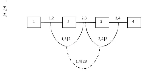
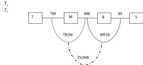
One of the simplest regular vine is shown in Figure 1. Here, T1 is the tree consisting of

the straight edges between the numbered nodes. T2is the tree consisting of the curved edges

that join the straight edges inT1, and so on. For a regular vine each edge of T1 is labelled

by two numbers from{1, ..., n}. If we take two edges ofT1 which become linked nodes inT2

then of the numbers labelling these edges one is common to both, and they both have one unique one. For example 12 and 23 are linked at the next level tree. The common number(s) will be called theconditioning setDefor that edgee(in this example the conditioning set is

simply{2}) and the other numbers will be called theconditioned set (in this example{1,3}). For a regular vine the conditioned set always contains two elements.

With such a vine we associate conditional copulas to each edge, to couple the two variables in the conditioned set given the values in the conditioning set.

Bedford and Cooke (2001) express a regular vine distribution in terms of its density in the following theorem.

Theorem 1 LetV= (T1, . . . , Tn−1)be a regular vine onnelements. For each edgee(j, k)∈

1

T

2

T

3

T

Figure 1: A regular vine with 4 elements

copula and copula density be Cjk|De andcjk|De respectively. Let the marginal distributions

Fi with densities fi, i= 1, . . . , n be given. Then the vine-dependent distribution is uniquely

determined and has a density given by

f(x1, . . . , xn) = n

Y

i=1

f(xi)

n−_Y1

j=1

Y

e(j,k)∈Ei

cjk|De(Fj|De, Fk|De) (2)

The existence of regular vine distributions is discussed in detail by Bedford and Cooke (2002).

The density decomposition associated with 4 random variables X = (X1, . . . , X4) with

a joint density function f(x1, . . . , x4) satisfying a copula-vine structure (this structure is

calledD-vine, see Kurowicka and Cooke, 2006, pp. 93) shown in Figure 1 with the marginal densitiesf1, . . . , f4 is

f1234(x1, . . . , x4) = 4

Y

i=1

f(xi)×c12{F(x1), F(x2)}c23{F(x2), F(x3)}c34{F(x3), F(x4)}(3) ×c13|2{F(x1|x2), F(x3|x2)}c24|3{F(x2|x3), F(x4|x3)}

×c14|23{F(x1|x2, x3), F(x4|x2, x3)}

This formula can be derived for this case using the general expression

f(x, y) =fX(x)fY(y)c(FX(x), FY(y)),

or equivalently

wherecis the copula density andFX, FY are the univariate distributions. Starting with

f1234(x1, . . . , x4) =f1(x1)f2(x2,|x1)f3(x3|x1, x2)f4(x4|x1, . . . , x3),

we inductively convert the latter expression into that shown in Equation 3. We have

f2|1(x2|x1) =f2(x2)c12(F1(x1), F2(x2)).

Next,

f3|12(x3|x1, x2) = f3|2(x3|x2)c13|2(F1|2(x1|x2), F3|2(x3|x2))

= f3(x3)c23(F2(x2), F3(x3))c13|2(F1(x1|x2), F3(x3|x2)).

The calculation forf4|123(x4|x1, . . . , x3) is left to the reader.

The above theorem gives us a constructive approach to build a multivariate distribution given a vine structure: If we make choices of marginal densities and copulae then the above formula will give us a multivariate density. Hence vines can be used to model general mul-tivariate densities. However, in practice we have to use copulae from a convenient class, and this class should ideally be one that allows us to approximate any given copula to an arbitrary degree. In the following sections, we address this issue in more detail. By having this class of copulae, we then can approximate any multivariate distribution using any vine structure.

Unlike the situation with Bayesian networks, where not all structures can be used to model a given distribution, the theorem shows that - in principle - any vine structure may be used to model a given distribution. However, in practice it seems that some vine structures do work better than others, and so this must be a result of restricting to a particular family of copulas. That is, given a family of copulae, some vine structures may give a better degree of approximation than others. In fact, we could say that the question “does a vine structure fit?” only makes sense in the context of a given family of copulae.

3

Building bivariate minimum information copulae

The emphasis on this paper is on approximation rather than on optimal estimation tech-niques. We use minimum information methods to demonstrate uniform approximation in the class of copulae used.

This section discusses some preliminary ideas that will be needed, and in particular shows how the approaches work to determine a unique copula when there are just two variables of interest.

3.1

Data: Expert judgment or random sample driven approaches

Quantitative models are typically parametrized either by expert judgement or estimation from data. Bedford and Cooke (2001), argue that expert judgement should be based on observable quantities. In our context, it is the uncertain quantities such as X that are observable. The quantileF(X) is a quantity could be argued to be an observable quantity if the distribution function F is known. Now the use of copulas implies that we must in fact know the marginal disributions, so this might not seem an important point. However, experts could normally be expected to find it easier to consider the joint behaviour of the untransformed variablesX1, X2, etc, than the joint behaviour of the transformed variables

F1(X1), F2(X2). Hence when using experts to make assessments it is definitely preferable

to use assessments on the untransformed variables. However, in the context of specifying joint distributions this causes more difficulties as there will generally be constraints. For example when two different marginal distributions are specified forX1X2, then the product

moment correlation might not be able to take values close to +/- 1. Fortunately, by working with minimum information distributions we can deal with this problem to some extent. This method allows interactive elicitation of expert opinions by giving guidance as to what values of uncertain quantities are compatible with the assessments already made (Bedford, 2006).

By contrast, when assessing distributions on the basis of data (large quantities of which may well be available for example in financial risk modelling problems), the data can be transformed to uniform after estimation of the marginals. This makes it possible to consider approximation, or encoding, of the data using a multivariate copula, and enables us to consider ways of judging how well that approximation can be made using given families of two-dimensional copulae. We shall consider two different approaches to do this.

3.2

The

D

AD

algorithm and minimum information copulae

Suppose there arekfunctions,h1, h2, . . . , hk: [0,1]2→R, for which we can specify the mean

valuesα1, . . . , αk that these functions should take. We seek a copula that has these mean

values, a problem which is usually either infeasible or underdetermined. Hence, assuming feasibility for the moment, we ask also that the copula be minimally informative (with respect to the uniform distribution), which guarantees a unique and reasonable solution: Define the kernel

A(u, v) = exp(λ1h1(u, v) +. . .+λkhk(u, v)). (4)

According to the general theory of Borwein et al. (1994), Nussbaum (1989) there is a unique copula with minimum information satisfying the constraints that the mean value of hi isαi (i= 1, ..., k), and this has density

d(1)(u)d(2)(v)A(u, v).

The parameters (λ1, . . . , λk) depend on (α1, . . . , αk) in a nonlinear way. Fortunately there are

numerical procedures to determine this relationship: Given (λ1, . . . , λk) we can determine the

functionsd(1)_{(u) andd}(2)_{(v) and then calculate the associated mean values forh}

We numerically solve this function to obtain the unique (λ1, . . . , λk) for which the mean values

ofh1, h2, . . . , hk areα1, . . . , αk.

The general theory says that the set of all possible expectation vectors (α1, . . . , αk) that

could be taken by (h1, h2, . . . , hk) under some probability distribution is convex, and that

for every (α1, . . . , αk) in the interior of that convex set there is a density with parameters

(λ1, . . . , λk) for which (h1, h2, . . . , hk) take these expectations.

This general approach to defining a copula was used by Bedford and Meeuwissen (1997) with a single functionh(u, v) =uv, which essentially measures the Spearman rank correlation of the copula. Bedford (2006) and Lewandowski (2008) have considered larger groups of functions.

The discrete version of this problem can be written in terms of matrices. Suppose that (u, v) are discretized into n points, respectively as ui, and vj, i, j = 1, . . . , n. Then we

write A = (aij), D1 =diag(d(1)1 , . . . , d (1)

n ), D2 =diag(d(2)1 , . . . , d (2)

n ), where aij = A(ui, vj),

d(1)i =d1(ui),d(2)j =d2(vj). The assumption of uniform marginals means that

∀i= 1, . . . n X

j

d(1)i d (2)

j aij = 1/n, and

∀j= 1, . . . n X

1

d(1)i d (2)

j aij= 1/n.

Hence

d(1)i =

n

P

jd

(2)

j aij

and d(2)j =

n

P

id

(1)

i aij

The problem of finding matrices D1 and D2 so that D1AD2 is a stochastic matrix has

been long studied. Sinkhorn and Knopp (1967) gave a simple algorthim, and the iterative proportional fitting algorithm (Cziszar, 1975) has been much used. IPF simply uses an iterative procedure to determine the entries of D1 andD2. The idea is very simple - start

with arbitrary positive initial matrices forD1 andD2. Then successively define new vectors

by iterating the maps

d(1)i 7→

n

P

jd

(2)

j aij

(i= 1, . . . , n), d(2)j 7→

n

P

id

(1)

i aij

, (j= 1, . . . , n)

This iteration converges geometrically to give us the vectors required.

Nussbaum (1989) considered the problem in much greater generality, considering contin-uous densities and functions, and showed that the corresponding functional is a contraction mapping on a space of functions endowed with a Hilbert projective metric. We shall make use of this fact when considering the quality of approximations made to copulae below.

3.3

Numerical construction of minimally informative copulae with

the

_D

_AD

algorithm

As discussed above, for a given set of functions (h1, . . . , hk), the mapping from the set of

vectors ofλ’s parameterizing the kernelAonto the expectations of the function (α1, . . . , αk)

has to be found numerically. We employ optimization techniques for achieving the result. We wish to determine the appropriate set ofλ’s for given expectationsαi, where the expectations

have been calculated using the discrete copula densityD1AD2.

Define

Ll(λ1, . . . , λk) :=

1 n2

n

X

i=1

n

X

j=1

d(1)(ui)d(2)(vj)A(ui, vj)hl(ui, vj)−αl, l= 1,2, . . . , k. (5)

We seek the roots of these functions. One of the possible solvers for this task would be FSOLVE - MATLAB’s optimization routine. It implements various root finding techniques allowing for choosing the one suiting our problem best. However we also obtained good results by using another of Matlab’s optimization procedures in the example below, namely FMINSEARCH, which implements the Nelder-Mead simplex method (Lagarias et al., 1998). The minimized function is

Lsum(λ1, . . . , λk) = k

X

l=1

L2l(λ1, . . . , λk).

As an example we show how an expert could specify a copula though defining two expected values.

Example 1 Suppose that we are given two uncertain quantitiesX andY with distribution functions FX and FY for which we want to specify a copula. Suppose that the marginal

distributions (these distributions can also be specified by an expert) are also ofX andY are as follows

X ∼N(0,1), Y ∼N(1,4)

In addition, suppose that an expert is willing to specify the expected values ofXY andX2Y, that is, the expected values of functionsh′

1(x, y) =xy,h′2(x, y) =x2y. We cannot directly

ap-ply the methods described above as these functions are given in terms ofX andY rather than the copula variables. But, we can find corresponding functions of the copula variablesU and V, defined byhi(u, v) =h′i(F

−1 X (u), F

−1

Y (v))(i= 1,2). The expected values of(h1, h2)under

the copula density equal the expected values of(h′

1, h′2)under the required joint distribution.

To numerically implement theD1AD2 algorithm we discretize the copula space by fixing

a size k of the square matrix kernel A and associate points in the unit square (ui, vj) with

each element of the matrix, where ui = (i−0.5)/k and vj = (j−0.5)/k. We then define

Aλ = exp{λ1h1(ui, vj) +λ2h2((ui)vj)}. The D1AD2 then gives us a discrete

approxima-tion to the copula with minimum informaapproxima-tion have a certain value ofE(XY)andE(X2_Y)

depending on the parameters λ1, λ2. Figure 2 shows the approximation of the copula for

0 0.2 0.4 0.6

0.8 1

0 0.5 1 0 0.5 1 1.5 2 2.5 3

U V

Figure 2: The minimally informative copula withλ1= 0.069806, λ2=−0.010728.

0 0.2 0.4 0.6

0.8 1

0 0.5 1 0 5 10 15 20

U V

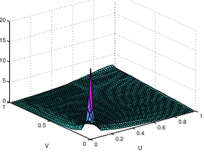
Figure 3: The minimally informative copula given the following constraints,E(XY) = 1 and E(X2_{Y) = 0.8.}

The functional relationship between the set of vectors of λ’s and the set of vectors or resulting expectations of functions of (h1, h2) can be determined numerically. Given the

expectations of the functions mentioned above fixed as follows, E(XY) = 1and E(X2Y) = 0.8, the optimal values for λ’s are: λ1 = 0.38893, λ2 = −0.11304. Figure 3 shows the

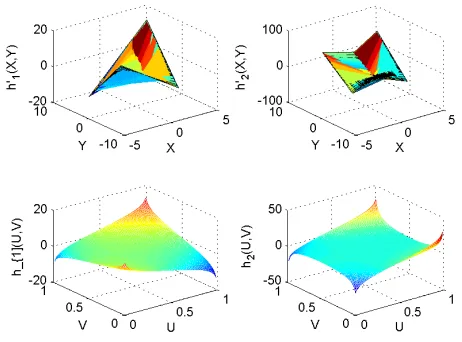
minimally informative (discretized) copula for these values. We also show both objective functions, (h′

1(X, Y), h′2(X, Y)) in Figure 4 together with their counterparts in the copula

space,(h1(U, V), h2(U, V)).

Figures 5, 6 show the expected values of h′

1(X, Y) and h′2(X, Y) as a functions of λ1

and λ2. We may wish to specify more expectation values. Figure 7 shows the minimally

informative copula given constraints on E(XY), E(X2_{Y), E(XY}2_{) and E(X}2_Y3_{) when}

Figure 4: Plots of base functions and the corresponding functions on the copula domain

0 0.2

0.4 0.6

0.8

−0.4 −0.3 −0.2 −0.1 0 0 0.2 0.4 0.6 0.8 1

λ

1

λ₂

E(XY)

Figure 5: The presentation ofE(XY) as a function of λ1 andλ2

0 0.2

0.4 0.6

0.8

−0.4 −0.3 −0.2 −0.1 0 0 0.2 0.4 0.6 0.8 1

λ

1

λ

2

E(X

2Y)

Figure 6: The presentation ofE(X2_{Y) as a function ofλ}

0 0.2

0.4 0.6

0.8 1

0 0.2 0.4 0.6 0.8 1 0 0.5 1 1.5 2 2.5

U Minimally informative copula given the experts’ assessments

V

Figure 7: The minimally informative copula given the following constraints: E(XY) = 0.1528,E(X2_{Y) = 0.9205,E(XY}2_{) = 0.1661 andE(X}2_Y3_{) = 13.5603.}

4

Copula compactness

One of the main aims of this paper is to show that we can arbitrarily well approximate a multivariate distribution by using a fixed family of bivariate copulae. A key step to demon-strating this is to show that the family of bivariate (conditional) copula densities contained in a given multivariate distribution forms a compact set in the space of continuous functions on [0,1]2_{. Based on this we can then show that the same finite parameter family of copulae}

can be used to give a given level of approximation to all conditional copulae simultaneously. It is worth defining more precisely the way in which we approximate densities. We assume that all densities are continuous. WriteC(Z) for the space of continuous real valued functions on a spaceZ, where we shall always takeZ = [0,1]r _{for somer. A norm on the space C(Z)}

is given by

||f1...r||= sup|f1...r(x1, . . . , xr)|.

Since our functions are assumed continuous on Z, and since Z is compact, the norm of any such function is finite. We shall be particularly interested in the set

C(f) ={cij|i1...ir : 1≤i, j, i1, . . . , ir≤n, i, j6=i1, . . . , ir}

wherecij|i1...ir is the copula of the conditional density ofXi, Xj givenXi₁, . . . , Xir. It will be

important to show that this set is relatively compact in the space of all continuous real valued functions C([0,1]2_{), because then we can show that the copula densities can be uniformly}

approximated. We consider compactness relative to the topology induced by the sup norm. Compactness of a setK can be defined equivalently through one of two properties, each of which we shall use:

2. Any sequence of points (which in our case are functions) ofK has a convergent subse-quence.

The famous Arzela-Ascoli Theorem gives another way of checking compactness when dealing with function spaces. It says that a subsetK⊂C([0,1]2_{) is relatively compact if the}

functions ofK are equicontinuous and pointwise bounded. We recall that a set of functions is equicontinuous if for allǫ >0 and (u, v) there is aδ >0 such that if the Euclidean distance

|(u, v)−(u′_{, v}′_{)|< δ then}

|g(u, v)−g(u′_{, v}′_{)|< ǫ ∀g∈K,}

and thatK is pointwise bounded if

sup{||g||:g∈K}<∞.

As a first step to showing the relative compactness ofC(f) we first give our attention to two other spaces: The set of conditional marginal densities

M(f) ={fi|i1...ir : 1≤i, i1, . . . , ir≤n, i6=i1, . . . , ir},

wherefi|i1...ir is the conditional density ofXi givenXi₁, . . . , Xir, and the set of conditional

bivariate densities

B(f) ={fij|i1...ir: 1≤i, j, i1, . . . , ir≤n, i, j6=i1, . . . , ir}

wherefij|i1...ir is the conditional density ofXi, Xj givenXi₁, . . . , Xir. Note that as we have

defined it, a member ofM(f) is a function of one variable - in other words, all the different marginals that we get for different conditions are individually members ofM(f). Similarly forB(f). Hence M(f)⊂C([0,1]) andB(f)⊂C([0,1]2_).

Theorem 2 The setsM(f)⊂C([0,1]) andB(f)⊂C([0,1]2_{)are relatively compact.}

Proof:

We have assumed that our multivariate density f1...n is a continuous function defined

on [0,1]n_{. Since all marginal densitiesf}

i₁...ir are obtained by integrating out variables from

f1...n, it is clear that

|fi₁...ir(xi₁, . . . , xir)| ≤sup|f1...n(x1, . . . , xn)|,

where the sup is taken over the variablesxi (i6=i1, . . . , ir). Hence

|fi|i₁...ir(xi|xi₁, . . . , xir)|=|

fii₁...ir(xixi₁, . . . , xir)

fi₁...ir(xi₁, . . . , xir)

| ≤ ||f||/α

In order to show equicontinuity we first note that each functionfi1...ir is uniformly

con-tinuous. Since there are only a finite number of such functions, we can always ensure that givenǫ >0 there is aδ >0 such that for anyi1. . . ir if

|(xi₁, . . . , xir)−(yi₁, . . . , yir)|< δ

then

|fi₁...ir(xi₁, . . . , xir)−fi₁...ir(yi₁, . . . , yir)|< ǫ.α.

Hence if|xi−yi|< δ then

|fi|i₁...ir(xi|xi1, . . . , xir)−fi|i₁...ir(yi|xi1, . . . , xir)| ≤ |fii₁...ir(xi, xi₁, . . . , xir)−fii₁...ir(yi, xi₁, . . . , xir)|/α≤ǫ

so thatM(f) must also be an equicontinous family.

A similar argument shows that B(f) is an equicontinous family.

¤

We can now show

Theorem 3 The setC(f)⊂C([0,1]2_{)is relatively compact.}

Proof

For any elementcij|i₁...ir ofC(f), we have

cij|i1...ir(ui, uj|xi₁. . . xir) =

fij|i1...ir(xi, xj|xi₁. . . xir)

fi|i1...ir(xi|xi₁. . . xir)fj|i₁...ir(xj|xi₁. . . xir)

.

Hence if we take a sequence of elements in C(f) then there are corresponding sequences of elements ofM(f) and B(f). Since M(f) is relatively compact there must be a convergent subsequence, and looking along that same subsequence there must be a subsequence of that for which the corresponding functions inB(f) converge. Now, along this subsequence the right hand side of the above expression converges, so the elements ofC(f) on this same sequence must converge (and to the same thing). In particular there is a convergent subsequence. HenceC(f) is relatively compact.

¤

Since all the functions inC(f) are positive and uniformly bounded away from 0 it follows that

Corollary 1 The set LN C(f) ={ln(g) :g∈ C(f)} ⊂C([0,1]2_{) is relatively compact.}

4.1

Linear bases and approximate copulae

The set C([0,1]2_{) can be considered a vector space, and in this context a basis is simply}

sequence of functions h1, h2, . . . ∈ C([0,1]2) for which any function g ∈ C([0,1]2) can be

written asg=P∞i=1λihi. There are lots of possible bases, for example

Given an ordered basis h1, h2, . . . ∈ C([0,1]2) and a required degree of approximation

ǫ >0 in the sup metric, we can consider the collection of open sets

Uk,ǫ={g∈C([0,1]2) : inf||g− k

X

i=1

λihi||< ǫ}

where the inf in the above definition is to be taken over all possible values of theλi. Now,

Uk,ǫ is clearly open and furthermore

Uk,ǫ⊂Uk+1,ǫ, ∞

[

k=1

=C([0,1]2).

So theUk,ǫ form an open cover ofLN C(f) and hence by definition of compactness there is

aksuch thatUk,ǫcoversLN C(f). We can state this as a result

Theorem 4 Givenǫ >0, there is aksuch that any member ofLN C(f)can be approximated to within errorǫ >0 by a linear combination ofh1, h2, . . . , hk.

The same result holds forC(f) (though not necessarily with the samek).

Finally, we remark that though we have been looking only at approximation in the sense of the sup norm, one could easily look at higher order approximation. For example, if we assume that the densityf1...n is continuously differentiable then all the derivatives are continuous

functions and the same arguments as used above show that they form an equicontinuous and pointwise bounded family. Following through we find that the copulae generated fromf1...n

are also continuously differentiable. By using a slightly different norm on the continuously differentiable functionsC1_([0,1]2_)⊂C([0,1]2_),

||g||1=||g||+|| d

dug||+|| d dvg||,

we can guarantee that a similar approximation result to the above holds with pointwise approximation of the derivatives as well.

4.2

Ensuring that approximating densities are copula densities

Since the approximations we make of a copula density might not be quite a copula density itself, we need to transform it to obtain a copula. This is done by weighting the density as described above in Section 3.2. If we have a continuous positive real valued functionA(u, v) on [0,1]2 _{then there are continuous positive functions d}

1(u) andd2(v) such that d1.d2.A is

a copula density, that is, it has uniform marginals. We call this density theC-Projection of Aand denote it C(A). It will also be convenient to denote by N(h) the normalization of a non-negative functionhwith finite integral.

Lemma 1 Letg be a non-negative continuous copula density. Givenǫ >0 there is aδ such that if||g−f||< δ then||g−C(f)||< ǫ.

Proof: We show that by takingf sufficiently close togone can ensure that the reweight-ing functions forf are as close to 1. This then implies thatC(f) is close tog.

Without loss of generality we can assume thatf is normalized. The proof uses the fact that we can use the Borwein-Lewis-Nussbaum approach to find functionsd1f(u) andd2f(v)

such thatd1f.d2f.f has uniform marginals. Such functions d1g and d2g exist also for g but

are constant ,d1g(u) =d2g(v) = 1. As discussed above, these reweighting functions are fixed

points of a functional that is a contraction mapping when using the Hilbert metricD_{on the}

appropriate space of pairs of functions (d1, d2).

We denote byLf the functional associated tof. Since this is a contraction mapping there

exists aλf ∈(0,1) such that

D_{(Lf(a, b), Lf(c, d))< λf}D_{((a, b),(c, d)).}

If we set a0 = 1, b0 = 1 and (an+1, bn+1) =Lf(an, bn), then we have convergence to the

required pair of functions (d1f, d2f) that reweightf to become uniform.

Now, by choosingfclose enough togwe can ensure two things. First that the contraction rate associated toLf is close to that ofLg, in particular less than some chosenλ <1. Second

we can ensure that

D_{(Lg(1,1), Lf(1,1)) =}D_{(1,1), Lf(1,1))}

is as small as required. This implies that

D_{((1,1),(a, b)) ≤} ∞

X

n=0

D_{((an, bn),(an+1, bn+1))}

≤ D_{((a0, b0),(a1, b1))} ∞

X

n=0

λn

= D((1,1), Lf(1,1))

1−λ .

Hence the reweighting functions forf are close to the identity, and soC(f) is close tog.

¤

Tim, according to Contraction Mapping Principle Theorem, if we let X = (d1n, d2n)be the appropriate space of pairs of functions(d1, d2), andLf(Lg) :X →X

be a contraction mapping with contractivity coefficient λf. Let x0 = (1,1) ∈ X

and inductively define(d1(n+1), d2(n+1)) =Lf(d1(n), d2(n)), n≥0. TheLf has a unique

fixed point(d1f, d2f), the sequence (d1(n), d2(n))converges to (d1f, d2f) and D_{((d1f, d2f),(d1(n), d2(n)))≤λ}n_fD_{((d1f, d2f),(1,1)).}

sequence. We remark that the reweighting functions have the same differentiability prop-erties as the functionf being reweighted. This can be seen from the integral equation that they satisfy:

d(1)(u) = R 1

d(2)_{(v)f(u, v)dv} and d

(2)_{(v) = R} 1

d(1)_{(u)f(u, v)du}.

5

Constructing approximations using minimally

infor-mative distributions

The above discussion has shown that we can approximate all conditional copulae using linear combinations of basis functions. We did not address the question of how you choose the appropriate parameter values, and indeed finding the parameters that would minimize the sup norm for a given copula is not of itself an appealing procedure. A pragmatic alternative that lies very close to the approach described above is to use the minimum information criterion. In other words given{1, h1, . . . , hk}: [0,1]2→Rwe seek values λ1, . . . , λk so that

exp(Pk1λihi) is close to the copula density we are approximating.

In the minimum information framework we do this by fitting the moments of hi. So if

R R

higdudv = αi then we search for the copula density with minimum information (with

respect to the independent distribution) that also has those moments. It can be shown that this copula density is unique and has the form

d1(u)d2(v) exp(

k

X

1

λihi(u, v)).

When we use a vine structure to model a multivariate distribution, the vine defines a decomposition of the multivariate distribution into certain conditional copulae, associated to the conditioned and conditioning sets of the vine. For example, if{i, j}is the conditioned set andDe is the conditioning set in one part of a vine, then the family of conditional copulae

forxi, xj givenDehas to be specified. Using the minimum information approach means that

we should specify mean values for the functionshrgiven the variables inDe, that is, we have

to specify the conditional meansαm(ij|De).

A multivariate distributions can be then approximated as follows:

• Specify a basis familyB(k)

• Specify a vine structure

• For each part of vine, specify either

1. meanα1, . . . , αk forh1, . . . , hk on each pairwise copula;

2. functionsαm(ji| De) for the mean values as functions of the conditioning

1

T

2

T

3

T

Figure 8: Selected vine structure for the Norwegian stock data set with 4 variables: Norwegian stock index (T), MSCI world stock index (M), Norwegian bond index (B) and SSBWG hedged bond index (S).

We illustrate the procedure by applying it to a financial data set.

Example 2 In this example, we use the same data set studied in Aas et al (2009). These are four time series of daily data: the Norwegian stock index (TOTX), the MSCI world stock index, the Norwegian bond index (BRIX) and the SSBWG hedged bond index, for the period from 0.4.01.1999 to 0.8.07.2003. We denote these four variables by T, M, B and S, respectively.

We want to generate vine approximation fitted to this data set to any given multivariate density using minimum information distribution. We select a similar vine structure with 4 elements shown in Figure 1 for this data presented in Figure 8. It should be noticed that, we can find the corresponding functions of the copula variablesX, Y, Z and W associated withT, M, B, S, respectively, defined byhi(X, Y) =h′i(F

−1

1 (X), F2−1(Y)), etc., and clearly

these should also have the same specified expectation, that is,E(h′

i(T, M)) =E(hi(X, Y)),

etc. The minimum information copulae calculated in this example are derived based on the copula variables,X, Y, Z, W.

We first can construct a minimally informative copula between any two variables joining together in the first tree, T1. As an example, we show the construction of a minimally

informative copula between two variables M and T denoted by CT M under the following

constraints: h′

1(M, T) = M T, h′2(M, T) =T M2, h3′(M, T) =T2M and h′4(M, T) =M T3.

In other words, we use the Fourier copula of order 4 or a base with 4 elements to approximate this copula. We fix the values of the expectations of these functions as follows

α1=

1 1094

1094_X

i=1

TiMi= 0.2314, α2=

1 1094

1094_X

i=1

0 0.2 0.4 0.6

0.8 1

0 0.5 1 0 0.5 1 1.5 2 2.5 3

X Minimally informative copula given the experts’ assessments

Y cTM

(X,Y)

Figure 9: The minimally informative copula betweenT andM variables of Norwegian Stock data.

α3= 1

1094

1094_X

i=1

Ti2Mi= 0.1465, α4= 1

1094

1094_X

i=1

Ti3Mi= 0.1058

The minimum information copulaCT M with respect to the uniform distribution given the

four constraints mentioned above has been constructed on the same grid of 50 by 50 equally spaced points and presented in Figure 9.

We now want to study the influence of adding more constraints on the approximation of the copula density. As we discussed above and as expected a minimum information copula should fit better to the data based on more constraints. We verify this point by fitting and comparing two minimum information copulae based on 3 and 12 constraints between variablesM andB.

We first use the Fourier copula of order 12 or a base with 12 elements to approximate the copula between variablesM and B, denoted byCM B. The selected objective functions for

this base are:

h′1(M, B) =M B, h′2(M, B) =B2M, h′3(M, B) =M2B, h′4(M, B) =M3B

h′

5(M, B) =M2B2, h′6(M, B) =M B3, h7′(M, B) =B2M3, h′8(M, B) =M2B3

h′9(M, B) =M3B3, h′10(M, B) =M B4 h′11(M, B) =M4B, h′12(M, B) =M5B

The minimum information copula CM B with respect to the uniform distribution given the

constraints above has been constructed on the same grid of 50 by 50 points. The constraints presented as the expectations of the objective functions and their Lagrange multipliers re-quired to construct the minimally informative copula betweenM andBare reported in Table 1.

The minimally informative copula density CM B given the constraints reported in Table

1 is presented in Figure 10.

The minimum information copulaCM Bwith respect to the uniform distribution and given

The Constraints The constraints approximated Lagrange based onCM B multipliers

E[h′

1(M, B)] = 0.2905 0.29026 26.2459

E[h′

2(M, B)] = 0.2075 0.20747 -27.4369

E[h′

3(M, B)] = 0.2066 0.20683 -3.3349

E[h′

4(M, B)1] = 0.1611 0.16122 -9.3389

E[h′

5(M, B)] = 0.1527 0.153 -0.3289

E[h′

6(M, B)] = 0.1624 0.16238 1.6079

E[h′

7(M, B)] = 0.1217 0.12181 25.9629

E[h′

8(M, B)] = 0.1223 0.1224 8.3688

E[h′

9(M, B)] = 0.0989 0.0988 -14.0917

E[h′

10(M, B)] = 0.1340 0.1338 6.5137

E[h′

11(M, B)] = 0.1324 0.1323 -17.0045

E[h′12(M, B)] = 0.1126 0.11228 10.1875

Table 1: The constraints, the approximated expectations, and their Lagrange multipliers to construct the minimal informative copula betweenM andB.

0.2905, E[h′

2(M, Z)] = 0.2075 andE[h′3(M, Z)] = 0.2066 has been constructed on the same

grid of 50 by 50 points, presented in Figure 11. Their Lagrange multipliers areλ1= 7.4845,

λ2= 2.3297 andλ3=−2.6631.

The log likelihoods of these two copulae based on 12 constraints and 3 constraints (and constructed on 200 by 200 grid points) are respectively: logL12pt

cM B = 92.1645 andlogL 3pt

cM B =

87.1966. This is in agreement with the point made above.

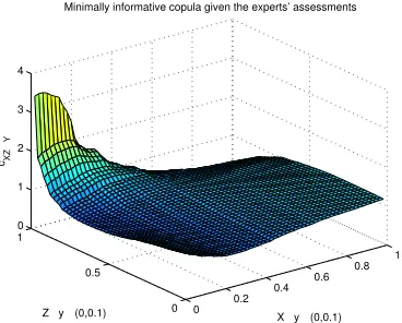
The conditional copulae in the second tree,T2can be similarly approximated based on the

minimally informative copula described above. We first construct the conditional minimum information copula betweenT |M andB |M given the following constraints represented as the conditional expectations of some objective functions:

h′1(T, B) =T B, h′2(T, B) =T B2, h′3(T, B) =T2B

To calculate this conditional copula, we divide the support of M into some arbitrary sub-intervals or bins (here, we use 10 bins), and we then compute the expectations of the afore-mentioned functions on each bin as the constraints. As a result, the minimum information copula C(T ,B)|M with respect to the uniform distribution and the following constraints on

the first bin, where 0< M <0.1

E[h′1(T, B)|M ∈(0,0.1)] = 0.1594, E[h′2(T, B)|M ∈(0,0.1)] = 0.0678,

E[h′

3(T, B)|M ∈(0,0.1)] = 0.1224

0 0.2 0.4 0.6

0.8 1

0 0.5 1 0 1 2 3 4 5

Y Minimally informative copula given the experts’ assessments

Z cMB

(Y, Z)

Figure 10: The minimally informative copula betweenM andBvariables of Norwegian Stock data based on 12 constraints presented in the first column of Table 1.

0 0.2 0.4 0.6

0.8 1

0 0.5 1 0 0.5 1 1.5 2 2.5 3

Y Minimally informative copula given the experts’ assessments

Z cMB

(Y, Z)

Bin The constraints Lagrange multipliers (E[h′

1|M], E[h′2|M], E[h3′ |M]) (λ1, λ2, λ3)

0< M <0.1 (0.1594, 0.0678, 0.1224) (10.9383, -8.4123, -6.9916) 0.1< M <0.2 (0.1785, 0.0857, 0.1252) (-4.2491, 8.1402, -5.2132) 0.2< M <0.3 (0.207, 0.1181, 0.1357) (2.1269,-1.7432,-1.4931) 0.3< M <0.4 (0.1891,0.1032,0.1171) (-7.2137,2.0704,1.9255) 0.4< M <0.5 (0.2587,0.1748,0.1653) (-8.7337,5.2627,3.8922) 0.5< M <0.6 (0.2377,0.1538,0.1526) (-12.5348,-1.6083,14.9014) 0.6< M <0.7 (0.2712,0.1802,0.1673) (3.9591,-7.3273,3.5925) 0.7< M <0.8 (0.2595,0.1736,0.1618) (7.3803,-15.482,8.9438) 0.8< M <0.9 (0.3156,0.2386,0.1945) (9.2597,-9.2321,-0.4385) 0.9< M <1 (0.2626,0.2087,0.1618) (-0.7429,-1.1895,0.6117)

Table 2: The constraints and corresponding Lagrange multipliers associated with the con-ditional minimal informative copula between T | M ∈ (0,1) and B | M ∈ (0,1) for each bin

0 0.2

0.4 0.6

0.8 1

0 0.5

1 0 1 2 3 4

X½ yÎ (0,0.1)

Minimally informative copula given the experts’ assessments

Z½ yÎ (0,0.1)

cXZ

½

Y

Figure 12: The minimally informative copula betweenT |M ∈(0,0.1) and B|M ∈(0,0.1) variables of Norwegian Stock data givenE[h′

1(T, B)|0< M < 0.1], E[h′2(T, B)|0 < M <

0.1], E[h′

0 0.2 0.4 0.6 0.8 1 0.1

0.15 0.2 0.25 0.3 0.35 0.4 0.45

y

E(XZ

½

y)

Lowerbound Mean Upperbound

Figure 13: The changes ofE[h′

1(T, B)|0< M <1] over the bins.

1 2 3 4 5 6 7 8 9 10 0

0.1 0.2 0.3 0.4 0.5 0.6 0.7 0.8 0.9 1

E(XZ

½

y)

y

Figure 14: Box-plot demonstration of theE[h′

1(T, B)|0< M <1].

Table 2 shows the constraints and the corresponding Lagrange multipliers required to build conditional minimum information copula betweenT | M ∈ (0,1) andB |M ∈(0,1) for 10 bins.

It is important to study the changes of the conditional expectation, E[h′

1(T, B) | M]

(E[XZ | y]) for different values of M or over the bins. Figure 13 shows this conditional expectation,E[h′

1(T, B)|M], calculated from the minimum information copulaC(T |M, B|

M) whereM varies on (0,1) along with the 95% confidence interval around the mean. As we can observe form this figure the changes of this measure is not...

The Box-plot demonstration of this conditional expectation,E[h′

1(T, B)|0< M <1] is

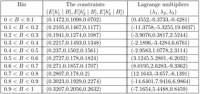
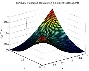
illustrated in Figure 14. Similarly, we construct the conditional minimum information copula between M | B and S | B given the following constraints represented as the conditional expectations of some objective functions:

h′1(M, S) =M S, h′2(M, S) =M S2, h′3(M, S) =M2S

Bin The constraints Lagrange multipliers (E[h′

1|B], E[h′2|B], E[h′3|B]) (λ1, λ2, λ3)

0< B <0.1 (0.1472,0.1098,0.0702) (0.4552,-0.3733,-0.4281) 0.1< B <0.2 (0.2105,0.1467,0.1177) (-11.3758,-5.3255,19.6037) 0.2< B <0.3 (0.1941,0.1274,0.1087) (-3.9076,0.3817,2.5244) 0.3< B <0.4 (0.2217,0.1493,0.1348) (-2.1896,-3.4284,6.6761) 0.4< B <0.5 (0.237,0.1502,0.1561) (-2.9583,1.0778,2.3114) 0.5< B <0.6 (0.2727,0.178,0.1824) (3.1245,5.2801,-6.2032) 0.6< B <0.7 (0.271,0.1857,0.1707) (8.0195,2.6283,-9.3362) 0.7< B <0.8 (0.2807,0.178,0.2) (12.1643,-3.657,-6.1391) 0.8< B <0.9 (0.3023,0.1929,0.2274) (-14.6401,7.9416,6.9864) 0.9< B <1 (0.3207,0.2056,0.2632) (-7.1654,5.4488,0.8459)

Table 3: The constraints and corresponding Lagrange multipliers associated with the con-ditional minimal informative copula between M | B ∈ (0,1) and S | B ∈ (0,1) for each bin.

bins (the bins are obtained by dividing the support ofB in 10 equal length sub-interval). Figure 15 shows this conditional expectation,E[h′

1(M, S)|B], calculated from the

min-imum information copula C(M | B, S | B) where B varies on (0,1) along with the 95% confidence interval around the mean. As we can observe form this figure the changes of this measure is not...

The Box-plot demonstration of this conditional expectation,E[h′

1(T, B)|0< M <1] is

illustrated in Figure 16.

The conditional minimally informative copula in the third tree, T3 can be similarly

ob-tained as described above. In this situation, we first divide the conditioning variables supports into some sub-intervals, and we then construct the minimum information copulaT |(M, B) and S | (M, B) given the some constraints represented as the conditional expectations of some objective functions where the conditioning variables varies over the specified bins. Fig-ure 17 shows a minimally informative copula betweenT | {M ∈ (0.33), B ∈ (0,0.33)} and S | {M ∈ (0.33), B ∈ (0,0.33)} with respect to the uniform distribution and given three constraints e1 =E[h′1(T, S) | y ∈ {M ∈ (0.33), B ∈ (0,0.33)}] = 0.394, e2 =E[h′2(T, S) | {M ∈(0.33), B∈(0,0.33)}] = 0.295, e3=E[h′3(T, S)| {M ∈(0.33), B∈(0,0.33)}] = 0.3115

which is constructed on the same grid of 50 by 50 data points. The objective functions used as the constraints are:

h′

1(T, S) =T S, h′2(T, S) =T S2, h′3(T, S) =T2S

Table 4 shows the constraints and corresponding Lagrange multipliers which enable us to construct the minimum information copula over the corresponding bin.

0 0.2 0.4 0.6 0.8 1 0.1

0.15 0.2 0.25 0.3 0.35 0.4 0.45

z

E(WY

½

z)

Lowerbound Mean Upperbound

Figure 15: The conditional expectationE[h′

1(M, S)|0< B <1] derived from the minimally

informative copula betweenM |B∈(0,1) andS|B∈(0,1) obtained above.

1 2 3 4 5 6 7 8 9 10

0 0.1 0.2 0.3 0.4 0.5 0.6 0.7 0.8 0.9 1

E(YW

½

z)

z

0 0.2

0.4 0.6

0.8 1

0 0.5

1 0 0.5 1 1.5 2 2.5 3

X½ yÎ (0,0.33), zÎ (0,0.33)

Minimally informative copula given the experts’ assessments

W½ yÎ (0,0.33), zÎ (0,0.33)

c_{X, W\mid (y\in (0, 0.33), z\in (0,0.33)

Figure 17: The minimally informative copula betweenT | {M ∈(0.33), B ∈ (0,0.33)} and S | {M ∈(0.33), B ∈(0,0.33)} variables of Norwegian Stock data given e1 =E[h′1(T, S)| {M ∈ (0.33), B ∈ (0,0.33)}] = 0.394, e2 = E[h′2(T, S) | {M ∈ (0.33), B ∈ (0,0.33)}] =

0.295, e3=E[h′3(T, S)| {M ∈(0.33), B∈(0,0.33)}] = 0.3115 constraints .

(E[h′

1(T, S)|M, B] Lagrange multipliers

Bins E[h′1(T, S)|M, B], (λ1, λ2, λ3)

E[h′

1(T, S)|M, B])

0.2 0.4

0.6 0.8

1

0.2 0.4 0.6 0.8 1 0.1 0.15 0.2 0.25 0.3 0.35 0.4 0.45 0.5

y z

E(XW

½

y,z)

Lowerbound

Mean

Upperbound

Figure 18: The conditional expectationE[h1(T, S)|0< M <1,0< B <1] derived from the

minimally informative copula betweenT | {M ∈(0,1), B∈(0,1)} andS| {M ∈(0,1), B∈

(0,1)}obtained above.

1,0 < B <1] (the middle plane and recognised by “O” in the figure) and 95% confidence bound (we use “+” to display the upperbound, and “♦” denotes the lowerbound) over the bins specified in Table 4.

6

Conclusion

In this paper, we present a novel method to approximate a multivariate distribution by any vine structure to any degree of approximation. Our approach uses the minimum informa-tion copulas that can be specified to any required degree of precision based on the data available. We prove rigourously that good approximation ‘locally’ guarantees good approx-imation globally. This approxapprox-imation allows the use of a fixed finite dimensional family of copulas to be used in a vine construction, with the promise of a uniform level of approxima-tion.In other words, we can use the same bases to approximate each copula in each tree of the corresponding vine.

distribution using a vine structure for a given multivariate copula depends on the bases represent the truncated class of copula and approximate levelǫ. This approximation can be made more accurate by adding more bases to achieve the desired level of approximationǫ.

We wish to extend our method by using a series expansion, like a two-dimensional Fourier series or generalized Fourier series, to approximate any log-density function by truncating the series at an appropriate point.

We are also considering the possibility of extending this work by using the emulators to estimate the expensive bases and therefore to approximate the resulting couples and vine.

References

[1] Aas, K., Czado, K. C., Frigessi, A., and Bakken, H. (2009). Pair-copula constructions of multiple dependence.Insurance, Mathematics and Economics,44, 182–198.

[2] Bedford, T. (2006). Interactive expert assignment of minimally-informative copulae.

[3] Bedford, T. and Cooke. R. M. (2001). Probability density decomposition for condition-ally dependent random variables modeled by vines.Annals of Mathematics and Artificial Intelligence 32, 245268.

[4] Bedford, T., and Cooke. R. M. (2002). Vines - a new graphical model for dependent random variables.Annals of Statistics, 30(4): 1031–1068.

[5] Bedford, T., and Meeuwissen, A. (1997). Minimally informative distributions with given rank correlation for use in uncertainty analysis.Journal of Statistical Computation and Simulation,57(1 - 4): 143 - 174.

[6] Borwein, J., Lewis, A., and Nussbaum, R. (1994). Entropy minimization, DAD problems, and doubly stochastic kernels.Journal of Functional Analysis, 123: 264–307.

[7] Joe, H. (1997). Multivariate Models and Dependence Concepts. Chapman & Hall, Lon-don.

[8] Knight, P. H. (2007). The Sinkhorn-Knopp Algorithm: Convergence and Applications. CERFACS Technical Report TR/PA/06/42, Strathclyde University Mathematics De-partment Technical Report 8-2006.

[9] Kurowicka, D., and Cooke. R. (2006).Uncertainty Analysis with High Dimensional De-pendence Modelling. John Wiley.

[10] Lagarias, J. C., Reeds, J. A., Wright, M. H., and Wright. P. E. (1998). Convergence pro- perties of the Nelder-Mead simplex method in low dimensions. SIAM Journal of Optimization,9(1):112–147.