Trajectory Optimization
Massimiliano Vasile
Department of Aerospace Engineering, University of Glasgow, James Watt South Building, G12 8QQ, Glasgow, UK
In this chapter we present a hybridization of a stochastic based search approach for multi-objective optimization with a deterministic domain decomposition of the solu-tion space. Prior to the presentasolu-tion of the algorithm we introduce a general formulasolu-tion of the optimization problem that is suitable to describe both single and multi-objective problems. The stochastic approach, based on behaviorism, combined with the decompo-sition of the solutions pace was tested on a set of standard multi-objective optimization problems and on a simple but representative case of space trajectory design.
1
Introduction
The design of a space mission steps through different phases of increasing complexity; generally, the first step is a mission feasibility study. In order to be successful, the feasi-bility study phase has to analyze, in a reasonably short time, a large number of different mission options. Each mission option requires the design of one or more trajectories that have to be optimal with respect to one or more criteria. In mathematical terms, the problem can be formulated as a search for multiple local minima, or as a multi-objective optimization problem.
In both cases, it is desirable to have a collection of several optimal solutions. Nor-mally in literature, single objective and multi-objective optimization are treated as two distinct problems with different algorithms developed to address one or the other (see [1, 3, 4, 5, 6, 7, 8] for some examples of algorithms for global single objective tion and [9, 10, 11, 12] for some examples of algorithms for multi-objective optimiza-tion). In most of the cases Evolutionary Algorithms seem to be the preferred method and many examples exist of their use to address both single objective and multi-objective problems in space trajectory design: Gage et al. has shown the effectiveness of genetic algorithms with niching technique compared to a simple grid search for the optimization of bi-impulsive transfers [13], Coverstone et al. used genetic algorithms for low-thrust trajectory design [15, 16], Gurfil et al. used niching genetic algorithms for the char-acterization of geocentric orbits [14], Vasile proposed a hybridization of evolutionary algorithms with SQP methods for the design of weak stability transfers [17] and an hy-bridisation with branch and bound for low-thrust trajectory design [18], and Dachwald et al. proposed the combination of a neurocontroller and of Evolutionary Algorithms for
C.-K. Goh, Y.-S. Ong, K.C. Tan (Eds.): Multi-Objective Memetic Alg., SCI 171, pp. 231–253.
the design of low-thrust trajectories[19]. More recently, an comparison of several global optimization methods applied to the optimization fo space trajectories showed that Dif-ferential Evolution outperforms GAs on some trajectory design problems [20, 21].
In general, all evolutionary-based approaches for global optimization implement some heuristic derived from nature. From the very basic evolutionary paradigms to the more complex behaviors of ant colonies or bird flocks, each one of these heuristics can be interpreted as basic behaviors (like reproduction, feeding or trail following) as-sociated to individual agents. This chapter presents a generalization of this concept: a population of agents is endowed with a set of individualistic and social behaviors, in order to explore a virtual environment composed of the solution space. The combina-tion of individualistic and social behaviors aims at an optimal balance between global search and local convergence (or exploration versus exploitation).
Furthermore, a unified formulation is proposed that can be applied to the solution of both multi-objective and single objective problems in which the aim is to find a set of optimal solutions, rather than a single one. In order to improve the exploration of the search space and to collect as many local minima as possible, the proposed meta-heuristic was hybridized with a domain decomposition technique.
2
General Problem Formulation
The general problem both for single and multi-objective optimization is to find a set X , contained in a given domain D, of solutions x such that the property P(x)is true for all x∈X⊆D,
X={x∈D|P(x)} (1)
where the domain D is a hyper-rectangle defined by the upper and lower bounds on the components of the vector x,
D=xi|xi∈[blibui]⊆ℜ, i=1, ...,n
(2) All the solutions satisfying property P are here defined to be optimal with respect to P, or P-optimal, and X can be said to be a P-optimal set. Now, the property P might not identify a unique set, for example if P is Pareto optimality, X can collect all the points belonging to a local Pareto front. Therefore we can define a global optimal set Xoptsuch that all the elements of Xoptdominate the elements of any other X ,
Xopt=
x∗∈D|P(x∗)∧ ∀x∈X⇒x∗≺x (3) where x∗≺x represents the dominance of the x∗solution over the x solution.
If we are looking for local minima, the property P is to be a local minimiser or a solution x∗can be said to dominate solution x if the associated value of the objective function f(x∗)<f(x). In this case Xopt would contain the global optimum or a set of global optima all with the same value of f .
In the case of multiple objective problems, given a set of solution vectors we can associate to each one of them a scalar dominance index Idsuch that:
where the symbol|.|is used to denote the cardinality of a set and Npis the set of the indices of all the given solution vectors. Here and in the following, a solution vector xi is said to be dominating a solution vector xj if the values of all the components of the objective vector f(xi)are lower than or equal to the values of all the components of the objective vector f(xj)and at least one component is strictly lower. In this case, for the j−th solution, P(xj)simply defines the property of being not-dominated by any other solution in the set Np, thus:
X={xj∈D|Id(xj) =0} (5)
For constrained problems, the property P is to be optimal, either locally or Pareto, and feasible at the same time. The property P can be expressed through a single scalar value or through a set of values and relationships. It can be a bolean value, a real number or a fuzzy expression (e.g. bad, average, good).
3
A Behavioral Prospective
The search for a set of solutions can be broken down to a three steps process: collecting information, making decision, taking action. For a black-box problem the collection of information is generally performed by sampling the solution space. The aim in this respect is to minimize the number of samples required to find the desired solution or set of solutions. The decision making process consists of deciding what action to take at every step of the search, selecting who does what in the case of multiple entities and deciding when to stop the search. The action step consists of implementing the selected actions by the selected entity. The three steps are required to be automatic with minimum human intervention, which means that the decision to orient the search in one or another direction should not require the human judgment (e.g. restrict the search space, increase the number of samples in a specific region).
Let us assume that a virtual agent is endowed with the ability of collecting pieces of information, making decisions and implementing actions. The decision making process could involve a long term planning of actions a closed-loop control mechanism or some sort of action-selection process in response to stimuli. For example in particle swarm optimization (PSO)[6] the velocity of each particle i is computed with a close-loop control mechanism:
vi+1=wvi+ui (6)
where w is a weight and given the random numbers r1,r2and the weights a1and a2the
control uihas the form:
ui=a1r1(xi−xgi) +a2r2(xi−xgo) (7) The search is continued till the decision to stop is taken. The control function requires a piece of information collected by the particle xgiand one collected by another particle xgo. In this case, the decision making process includes the selection of the particle in xgo.
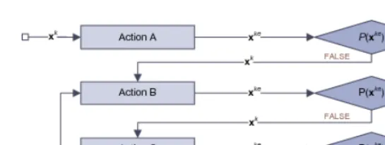
Fig. 1. Example of action selection mechanism
as individualistic, since involve only one agent at time, while others as social since re-quire interaction among multiple agents. A collection of actions and the action selection process define a behavior. When at step k an agent xkimplements an action, it produces an outcome xke according to:
xke=xk+β(xk,xk−1,Π
k,Al) (8)
whereβ is a function of the current state of the agent xk, the current state of the popu-lationΠk, the past state of the agent xk−1and the information about the past state of the population stored in an archive Al. Note thatβ is not analytical but is an algorithm that selects an action, assigns a value and return a variationΔxk.
For example, for individualistic behaviors (see Fig. 1 and the next section), each agent can perform three types of actions, A, B and C. This general scheme accommo-dates two types of heuristics: Action A generates always the same outcome every time is performed once a solution vector x is given (e.g. inertia in PSO), while Actions B and C generate different values for the same x every time they are performed (e.g. mutation in EA[1]). These last two actions are repeated until an improvement is registered or a maximum number of attempts is reached. The index keis increased by one every time an action is performed, and every action makes use of the agent status x, the status of other agents and of the outcome of the proceeding actions.
4
MultiAgent Collaborative Search
A population of virtual agents (i.e., points within H)is deployed in the search space:
H= [a1,b1]× ··· ×[an,bn]
of actions, derived from PSO, EA and Differential Evolution (DE)[4] and very simple, basic action selection mechanisms. The general scheme both for a single agent and for a group is: select actions, implement actions, evaluate actions, make decision.
Given an agent x∈H, a hyperrectangle
Sx=Sx1× ···Snx
is associated to it, where each Sx
i is an interval centered at the corresponding component x[i]of the agent. The size of Sxis specified by the valueρ(x): the i-th edge of Sxhas length
2ρ(x)max{bi−x[i],x[i]−ai).
As we will see, theρvalue associated to an agent is updated at each iteration according to some rule (see Section 4.2.1). The intersection Sx∩H basically represents the local region around agent x which we want to explore. We also associate an effort value s(x)to each agent x, which specifies the amount of computational effort we want to dedicate to the exploration of Sx. This value is updated at each iteration (see, again, Section 4.2.1).
The subdomain H is explored locally by acquiring information about the landscape within each region Sxand explored globally by evolving a population of agents which
are also allowed to collaborate with each other. Moreover, an archive Al of solutions over the domain H is maintained during the search. The archive is maintained in order to have a set of solutions for the problem at hand (see the discussion in the Introduction). The proposed approach, called Multiagent Collaborative Search (MACS), is outlined in the following, while the details will be specified in the following subsections.
Multiagent Collaborative Search
Step 0. Initialization. Generate an initial population of agentsΠ0 within H through
a Latin Hypercube (i.e., a non-collapsing design where points/agents are evenly spread even when projected along a single parameter axis; for a more detailed de-scription and a justification of the use of Latin Hypercubes we refer, e.g., to [22]). A hyperrectangle Sx0j is associated to the j-th agent x0
j∈Π0. The initial sizeρ(x0j)of each region Sx0j is fixed to 1 (i.e., the initial local region of each agent corresponds
to the whole set H). The effort s(x0j)dedicated to agent x0j∈Π0is fixed to the same
value smax(equal to n in the computations) for all agents inΠ0. Set k=0.
Step 1. Social Behavior. A set of social actions, specified by a social behavior are ap-plied to the populationΠk. In particular two sets of social actions are implemented: • Collaboration. The agents exchange information with each other. Each set of communication actions gives rise to new sampled points. Some of them identify the new location of a subset of the collaborating agents. See Section 4.1.1. • Repulsion. If two or more agents are too crowded one or more are reallocated
in the search space. See Section 4.1.2.
Step 2. Filtering. A filter partitions populationΠkinto two subsetsΠkin, the population within the filter, andΠout
k , the population outside the filter. See Section 4.3. Step 3. Individualistic Behavior. A set of individualistic actions, specified by an
• Local Exploration. These set of actions allows local exploration (within Sx) of the region around the agent. They are repeatedly applied until either an im-provement is observed or the number s(x)of actions is reached. If an agent x generates an improvement, populationΠkis updated by replacing x with its improvement. See Section 4.2.
• Hyperrectangle and effort update. The size parameterρand the effort parameter s associated to each agent within the filter are updated according to some rule. See Section 4.2.1.
Step 4. Archive update. Apply filtering and update archive Al(see Section 4.4). Step 5. Stopping rule. A stopping rule is checked (see Section 4.5). If it is not
sat-isfied, then set k=k+1 and go back to Step 1. If it is satisfied, then update the archive Alby adding the current population, i.e., set Al=Al∪Pk.
4.1 Social Behavior
Social behavior is defined through a set of communication actions (collaboration), a de-cision making process to select the outcome of the communication actions, a repulsion mechanism to limit crowding and increase diversity and a shared memory mechanism to exploit the social knowledge acquired during the search.
4.1.1 Collaboration
Collaboration defines operations through which information is exchanged between pairs of agents. Given a pair of agents x1 and x2, with x1 considered to be the better one
according to property P, three different actions are defined. Two of them are defined by adding to x1a stepΔξ defined as follows
Δξ =α2rt(x2−x1) +α1(x2−x1),
and correspond to: extrapolation on the side of x1 (α1=0, α2=−1, t =1), with
the further constraint that the result must belong to the domain H (i.e., if the stepΔξ leads out of H, its size is reduced until we get back to H); interpolation (α1=0,α2=
1), where a random point between x1and x2is sampled. In the latter case, the shape
parameter t is defined as follows:
t=0.75s(x1)−s(x2) smax
+1.25
The rationale behind this definition is that we are favoring moves which are closer to the agent with a higher fitness value if the two agents have the same s value, while in the case where the agent with highest fitness value has a s value much lower than that of the other agent, we try to move away from it because a small s value indicates that improvements close to the agent are difficult to detect.
generate two new solutions. Note that the three operations give rise to four new samples, denoted by y1, y2, y3, y4.
The first of the two parent agents is selected at random in the worst half of the current population (from the point of view of the property P), while the second parent is selected at random from the whole population. Selecting the first parent from the best half generally reduces the diversity of the population and may cause premature convergence.
Note that here all the communication actions are selected and implemented sequen-tially. However, according to the general scheme mentioned above, a different action selection mechanism can adaptively choose the most appropriate subset of actions at every step. The decision making process is used to select which of the four samples will be used. Each pair of parent agents x1and x2generates four samples y1, y2, y3and
y4. Then, a tournament, based on the property P, is started between the worst of the two
parents and the best of the four samples. The winner of the tournament will be the new location in the solution space of the worst parent agent. When an agent is displaced no update ofρand s is performed.
4.1.2 Repulsion
When the distance between two agents drops below a given threshold, a repulsion action is applied to the one with the worst P. More precisely, consider agent xjand let
Mj={i : Sxj∩Sxi=/0}
be the set of agents whose box has a nonempty intersection with the one of xj. Let nc(j) denote the cardinality of Mj. Then, for each i∈Mjwe check the following condition
wcnc(j)ρ(xj)>ρi j,
whereρi jdenotes the normalized distance1between xiand xjand wcis a small positive parameter called crowding factor. If the condition is satisfied, then the worse between agents xiand xj is repelled (note that wc=0 corresponds to no repulsion). Repulsion is basically an interpolation between the agent to be repelled and one vertex of the current domain chosen at random. The idea behind repulsion is to avoid convergence of different agents to the same subregion with a consequent waste of computational effort.
4.1.3 Shared Memory
The archive Al is used to direct the movements of those agents for which P is false. For all agents for which the property P is not true at step k the inertia component is recomputed as:
Δξ =r(xAl−x
k)
(9) where xAl is an element taken from the archive. The elements in the archive are ranked
according to their relative distance or crowding factor. Then, every agent for which P is false picks the least crowded element xAl not already picked by any other agent.
1By normalized distance we mean the distance between the two agents once H has been
4.2 Individualistic Behavior
The individualistic behavior is defined through a set of local exploration actions, an action selection mechanism, a decision making process to select the outcome of the exploration and an adaptive update of the resources and of the regions Sx.
At every generation, a behaviorβ is used to generate the set of exploration actions. In particular, given agent j at generation k, denoted by xkj, a behavior is a collection of displacement vectorsΔξ generated by some function zβ:
β={Δξ |xkj+Δξ ∈H andΔξ=zβ(xkj,xkj−1,w,r,Πk)} (10)
where zβ is a function of the current and past state xkj and xkj−1of agent j, of a set of weights w, of a set of random numbers r and of the current population Pk. Every point xkj+Δξ is called a child of agent j. In what follows we describe the different kinds of actions employed in this chapter.
Inertia. This action is performed at most once at each generation. If agent j has im-proved from generation k−1 to generation k, then we follow the direction of the improvement (possibly until we reach the border of the hyperrectangle associated to the agent), i.e., we perform the following step:
Δξ=λ¯(xkj−xkj−1) (11)
where
¯
λ =min{1,max{λ : xkj+λ(xkj−xkj−1)∈Sxj}}.
Follow-the-trail. This step is inspired by Differential Evolution (see, e.g., [8, 4]). It is defined as follows: let xki1,xki2,xki3 be three randomly selected agents; then
Δξ =xkj−(xki1+ (x
k i3−x
k
i2)) (12)
(if the step leads out of Sxj, then its length is reduced until we reach the border of Sxj).
Random-Walk. Given the agent x and its associated hyperrectangle Sx, four different
kinds of mutation actions are performed all arising from the following displacement of a component i of the agent:
Δξi=w1rt(i−xi) + (1−w1)rt(ui−xi) (13)
whereiand uiare respectively the lower and upper limits of xiwithin Sx∩H, r is a uniform random number in[0,1], w1=1 with some probability piand w1=0 with
probability 1−pi, and t ≥0 is a shape parameter (t=1 corresponds to uniform sampling, while t>1 favors more local moves). The four mutation actions are the following:
• all components i are perturbed according to (13) with t=1 and pi=0.5; • a component i is selected at random and perturbed according to (13) with t=1
and pi=0.5;
• a component i is selected at random and randomly fixed either at its lower limit or its upper limit in the region Sx∩H, i.e., t=0 and pi=0.5.
Linear blending. Once a mutation action on agent x has been performed, its result, denoted by y, is further refined through blending procedures. Linear blending cor-responds to the following displacement:
Δξ=α2rt(y−x) +α1(y−x). (14)
whereα1,α2∈ {−1,0,1}, r∈[0,1]is a random number, and t a shaping parameter
which controls the magnitude of the displacement. Here we use the parameter val-uesα1=0,α2=−1, t=1, which corresponds to extrapolation on the side of x,
andα1=α2=1, t=1, which corresponds to extrapolation on the side of y. If the
displacement defined by an extrapolation action is too large, i.e., the resulting point is outside the hyperrectangle associated with the current agent, then it is reduced until the resulting point is within the hyperrectangle.
Quadratic blending. The outcome of the linear blending can be used to construct a second order local model of the fitness function. We can define a second order blending operator that generates a displacement using the agent x, the perturbation y obtained by mutation, and the new point z generated by the linear blending oper-ator. A second order one-dimensional model of the fitness function along the line with direction x−z is obtained by fitting the fitness values in the three points x, y and z. Then, the new point is the minimum of the second-order model along the intersection of the line with the hyperrectangle associated with the agent.
As already pointed out, the inertia action is performed at most once. All the other actions are cyclically performed until either an improvement is observed or the number s(xkj) of actions is reached. Note that in each cycle only one of the four mutation actions is performed in turn.
4.2.1 Size and Effort Update
Given an agent xkj∈Πkin, its size parameterρ(xkj), defining the hyperrectangle Sxkj
cen-tered at xkj, and its effort parameter s(xkj), giving the maximum number of actions ap-plied to it, are updated at each generation. Both are reduced or enlarged depending on whether an improvement has been observed or not in the previous generation.
If xkj+1=xkj, i.e., an improvement has been observed for agent j at iteration k, then the effort is updated according to the following formula:
s(xkj+1) =max{s(xkj) +1,smax},
i.e., it is increased by 1, unless the maximum allowed number of actions has been al-ready reached (recall that in the computations smaxhas been fixed to the dimension n of
the problem). Basically, we are increasing the effort if the agent is able to improve. In the same case the size is increased by the following formula:
where rank(xkj+1)is the ranking of the agent xkj+1within the populationΠk (the best individual has rank equal to 1, the second best equal to 2, and so on). Basically, the worse the ranking of an individual, the greater the possible increase of the radius will be. The increase is limited from above by 1 (whenρ=1 the local region around the agent to be explored is equal to the whole domain H). The idea is that for low ranked individuals it makes sense to look for larger improvements and then to try to find a better point in larger regions making the search more global.
If no improvement is observed, then the effort is updated according to the following formula:
s(xkj+1) =max{s(xkj)−1,1},
i.e., it is decreased by 1, unless the minimum allowed number of actions has been al-ready reached.
In the same case the size is reduced according to the following rule. Letρmin(xkj)be the smallest possible reduction of the size parameter such that the child y∗of xkj with best fitness value is still contained in the hyperrectangle. Then:
ρ(xkj+1) =
ρmin(xkj) if ρmin(xkj)≥0.5ρ(xkj) 0.5ρ(xkj)otherwise
i.e., the size parameter is reduced toρmin(xkj)unless this is smaller than 0.5ρ(xkj), in which case we only halve the size parameter.
4.3 Filtering
Given a populationΠk, a filter simply subdivides the population into two parts,Πkin andΠkout.Πkincontains the best members of the populationΠk, i.e., those with the best fitness values, whileΠkoutcontains all the other individuals inΠk. The main difference between agents inside and outside the filter is that on agents outside the filter, only mu-tation actions (see equation (13) below) over the whole subdomain H are performed (for each agent outside the filter the number of these mutation actions is a random one between 1 and the size ofΠout
k ), while also other actions, allowing a deeper local exploration, are performed on agents inside the filter (see the following Section 4.2). Moreover, values ρ and s are only updated for agents in Πin
k (see the following Section 4.2.1). In the case an agent outside the filter at iteration k enters the filter at iteration k+1, itsρand s values are initialized as specified in Step 0.
4.4 Archive Update
Letρtol be a small threshold value, xi be an agent whose size parameter is below the threshold value, i.e.,ρ(xi)<ρtoland Libe the set of agents whose normalized distance from xiis below the thresholdρtol (including xiitself). If agent xi is the best one in
4.5 Stopping Rule
The stopping rule is quite simple: the search within a subdomain is stopped when a prefixed number Neof function evaluations is reached.
4.6 Definition of P for Multiobjective Optimization
Although the problem formulation through the definition of P is general and applica-ble to both single objective and multiple objective optimization proapplica-blems, either con-strained or not, the actual property is substantially different depending on the type of problem.
For box constrained multi-objective problems the property P can be defined by the value of the scalar dominance index Id, thus:
Id(x)>Id(xke) +ε⇒P(xke) =true (15)
whereεis now the minimum expected improvement in the computation of the domi-nance. Note that this easily accommodates the concept ofεdominance.
Now, when multiple outcomes with the same dominance index are generated by either social or individualistic actions, the one that corresponds to the longest vector difference in the criteria space with respect to x is considered. Note that in many sit-uations the action selection scheme in Fig. 1 generates a number of solutions that are dominated by the agent x. Many of them can have the same dominance value; therefore in order to rank them, we use the modified dominance index:
Id(x) =
j| fj(xke) =fj(x)
κ+
j| fj(xke)>fj(x)
(16)
whereκis equal to one if there is at least one component of f(x)=[f1,f2, ...,fNf]
Twhich is better than the corresponding component of f(xke), and is equal to zero otherwise.
Now, if for the kethoutcome, the dominance index in Eq.16 is not zero but is lower than the number of components of the objective vector, then the agent x is only partially dominating the kethoutcome. Among all the partially dominated outcome with the same dominance index we chose the one that satisfies the condition:
min ke
f(x)−f(xke)
,e (17)
where e is the unit vector of dimension Nf, e=[1,1,1,...,1]
T
√
Nf , and Nf is the number of
objective functions.
Since the partially dominated outcomes of one agent could dominate other agents or the outcomes of other agents at the end of every evolution cycle all the outcomes are added to the archive. Then, the dominance index in Eq.4 is computed for all the elements in Aland only the non-dominated ones are preserved.
4.7 Hybridization with Domain Decomposition
exhaustiveness of the search, MACS is combined with a deterministic domain decom-position technique. The search space D, is a hyperrectangle and the subdomains into which it is subdivided are also hyperrectangles. The stochastic algorithm searches on the subdomains in order to evaluate them. In this section we will give the details of the deterministic method.
Below we give the description of a generic branching procedure for GO problems. BRANCHING PROCEDURE
Step 0. Initialization LetF ={D}.
Step 1. Node selection Letθbe a function which associates a value to each node H∈ F. Then, select a node H∈F such that
H∈arg min
H∈Fθ(H), (18)
Step 2. Evaluation Evaluate the selected node H through some procedure.
Step 3. Node branching Subdivide H intoη nodes Hi, i=1, . . . ,η, for some integer η≥2, and updateF as follows:
F= (F\ {H})∪ {H1, . . . ,Hη}.
Step 4. Node deletion Delete nodes fromF according to some rule. Step 5. Stopping rule IfF =/0, then STOP. Otherwise, go back to Step 1.
Note that in the scheme above each node corresponds to a subdomain, and in what follows the two terms will be used as synonymous. Such scheme is quite typical for branch-and-bound methods. For these methodsθ delivers a lower bound for each sub-domain; each node is evaluated by evaluating feasible points within the corresponding subdomain (if any) and possibly updating the upper bound; node branching can be performed in several ways; node deletion is done through standard fathoming rules. However, what is missing in our context is an easy way to obtain bounds. Therefore, while we retain the branching structure, we need some other ways to define a function θ and to evaluate, branch and delete nodes. All this will be specified in the following subsections.
4.7.1 Node Evaluation
The evaluation of a subdomain H is done by running the MultiAgent Collaborative Search (MACS) algorithm within H. The MACS algorithm explores the subdomain H and stores in a local archive Al all the promising points in H. The local archive Al is then compared to the global archive Agcontaining all the points in the search space for which P is true. The points in Ev(H) = (Al∩Ag)∩H represent the evaluation of the subdomain.
4.7.2 Node Branching
H= [a1,b1]× ··· ×[an,bn]
be the domain to be subdivided. Let
j∈arg max i=1,...,n
bi−ai
Di−di
,
where diand Didenote respectively the lower and upper bounds for variable xiin the original domain D. We can now subdivide the interval bi−ai into a number nj of subintervals and look for the one that contains the majority of the points in H. Now if the subinterval has boundaries bik and aik with k=1, ...,nj, the cutting point ˜xj is defined as:
˜ xj=
bikif (bi−bik)>(aik−ai)
aikif (bi−bik)≤(aik−ai) Then, we define the two new subdomains
H1= [a1,b1]× ···×[aj,x˜j]× ···×[an,bn],
H2= [a1,b1]× ···×[x˜j,bj]× ···×[an,bn].
4.7.3 The Game of Exploration
The selection of the subdomain H on which to perform a new search with MACS de-pends on the outcome of a simple game between two players: explorer and exploiter.
Before presenting the game and selection process, we need to introduce two other functionsω andϕ. Let H be a given subdomain and ˜H be its father. Functionω is defined as follows for H:
ω(H) =max{N(H),1} N
(D)
(H) (19)
where(·)denotes the geometric mean of the edge lengths of an n-dimensional hyper-rectangle, N is the number of points in Ev(H)˜ , obtained through the evaluation of the father node ˜H by the MACS algorithm, and N(H)is equal to the number of points in Ev(H)˜ which also belong to H, i.e., N(H) =|Ev(H)˜ ∩H|(for the root node D we sim-ply set N(D) =N). We also remark that in (19) the ratio between geometric means of the edge lengths can also be viewed as the nth root of a ratio between volumes:
(D)
(H)=
Vol(D) Vol(H)
1 n
.
Then, small values forωare obtained for subdomains with small N(H)and large vol-ume, i.e., for subdomains with a low density of observed points. Functionϕ is defined as follows:
ϕ(H) =|{i|I(xi) =0}| (20)
always tries to maximize convergence and thus selects always the subdomain with the highest value ofϕ. If both players play explore (explore-explore strategy), then the al-gorithm will select the subdomain with the smallestω for further exploration, if both players play converge (converge-converge strategy), then the algorithm will select the subdomain with the highestϕ. If explorer plays explore first and exploiter plays con-verge (explore-concon-verge strategy) then, the algorithm will rank the subdomain accord-ing toωand then, among the first nωof them will take the one with the largest number of elements in Al. Vice versa, if exploiter plays first (converge-explore strategy), the algorithm will rank the subdomains according toϕ and among the first nϕ will select the one with the lowestω. The selection of the strategy to play depends on the outcome of the game.
If both players play converge then exploiter gets a reward only if it finds an improve-ment while explorer gets no reward whatsoever. Since we are interested in collecting as many different elements of a set as possible, this strategy is not convenient for any of the two players. If both players play explore then the explorer gets a reward while the exploiter gets half of the reward of the explorer only if an improvement is registered. This strategy is convenient if no improvements are registered with any other strategy or if no information is available. Thus, it is the first strategy that both players play at the beginning. The outcome of the exploration of a subdomain could be: a) a number of points belonging to the set X higher than the one already available, b) a number of points belonging to the set X lower or equal to the number already available, c) no points belonging to the set X . In the last case the algorithm plays explore-explore, in case a) though the subdomain looks promising the higher number of points could suggest an over-exploitation of the subdomain and the algorithm then plays explore-converge. Fi-nally, in case b) the algorithm plays converge-explore.
4.8 Discussion
The hybrid behavioral-based approach presented in the previous sections is one possible implementation of the concept expressed by Eq.8. In particular we used a very simple action selection mechanism for both social and individualistic actions. More sophisti-cated mechanisms may allow for a reduction of the number of function evaluations or could include a learning mechanism. Furthermore, in the present implementation there is a limited use of the past history of the search process. The behavior Eq.8 depends on the archive Al, which works as a repository of the social knowledge, and on the state of the agent at step k−1, therefore only a partial history is preserved and used.
4.9 Preliminary Optimization Test Cases
The proposed optimization approach, combining MACS with deterministic domain de-composition, was implemented in a software code in Matlab called EPIC, and tested on a number of standard problems, well known in literature. In a previous work [24, 25], EPIC was tested on single objective optimization problems related to space trajectory design, showing good performances.
Table 1. Multiobjective test functions
Scha f2= (x−5)2; f1=
⎧ ⎪ ⎪ ⎨ ⎪ ⎪ ⎩
−x i f x≤1
−2+x i f 1<x<3 4−x i f 3<x≤4
−4+x i f x>4
x∈[−5,10]
Deb f1=x1 x1,x2∈[0,1]
f2= (1+10x2)
1−
x1
1+10x2 α
− x1
1+10x2sin(2πqx1)
α=2;. q=4 T4 g=1+10(n−1) +∑ni=2[x2
i−10cos(2πqxi)]; x1∈[0,1]; h=1−
f1
g xi∈[−5,5];
f1=x1; f2=gh i=2, . . . ,n
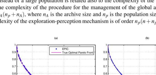
The test case, T4, is commonly recognized as one of the most challenging problems since it has 219different local Pareto fronts of which only one corresponds to the global Pareto-optimal front. In this case the exploration capabilities of each single agents are enough to locate the correct front with a very limited effort. In fact even with just five agents it was possible to reconstruct (see Fig. 2b) the correct Pareto front 20 times over 20 different runs. The total number of function evaluations was fixed to 20000 for each of the runs, though already after 10000 function evaluations EPIC was always able to locate the global front (see Fig. 2a).
Despite the small number of agents the sampled points of the Pareto are quite well distributed with just few and limited interruptions. The use of a limited number of agents instead of a large population is related also to the complexity of the algorithm. In fact the complexity of the procedure for the management of the global archive is of order nA(np+nA), where nAis the archive size and npis the population size, while the com-plexity of the exploration-perception mechanism is of order np(n+np), therefore, even
0 0.2 0.4 0.6 0.8 1
0 0.1 0.2 0.3 0.4 0.5 0.6 0.7 0.8 0.9 1 f 1 f2 (a) EPIC
True Optimal Pareto Front
0 0.2 0.4 0.6 0.8 1
0 0.1 0.2 0.3 0.4 0.5 0.6 0.7 0.8 0.9 1 f 1 f2 (b)
Fig. 2. Pareto front for the test case T4: a) 10000 function evaluations, b) 20000 function
[image:15.512.57.379.398.553.2]Table 2. Comparison of the average Euclidian distances between 500 uniformly space points on
the optimal Pareto front for various optimization algorithms
Approach T4 Scha Deb
EPIC 1.542e-3 (5.19e-4) 5.4179e-4 (1.7e-4) 1.4567e-4 (3.61e-4) NSGA-II 0.513053 (0.118460) 0.002536 (0.000138) 0.001594 (0.000122) PAES 0.854816 (0.527238) 0.002881 (0.00213) 0.070003 (0.158081) MOPSO 0.0011611 (0.0007205) 0.002057 (0.000286) 0.00147396 (0.00020178)
if the algorithm is overall polynomial in population dimension, the computational cost would increase quadratically with the number of agents.
As an additional proof of the effectiveness of MACS, we compare the average Eu-clidean distance of 500 uniformly spaced points on the true optimal Pareto front from an equal number of points belonging to the solution found by EPIC, NSGA-II, PAES and MOPSO (see Table 2).
5
Application to Space Trajectory Design
In this section we present an apparently very simple example of space trajectory opti-mization. It is a two impulse transfer from the Earth to the asteroid Apophis. As it often happens, the goal is to minimize the propellant consumption and the time of flight. The cost of the mission, in fact, increases proportionally to both quantities.
The propellant consumption is a function of the velocity change, orΔv[23], required to depart from the Earth and to rendezvous with Apophis. Both the Earth and Apophis are point masses, with the only source of gravity attraction being the Sun. Therefore, the spacecraft is assumed to be initially at the Earth, flying along its orbit. The first velocity change, orΔv1, is used to leave the orbit of the Earth and put the spacecraft
into a transfer orbit to Apophis. The second change in velocity, orΔv2, is then used to
inject the spacecraft into Apophis’ orbit.
The twoΔv’s are a function of the positions of the Earth and Apophis at the time of departure t0and at the time of arrival tf =t0+T , where T is the time of flight. The
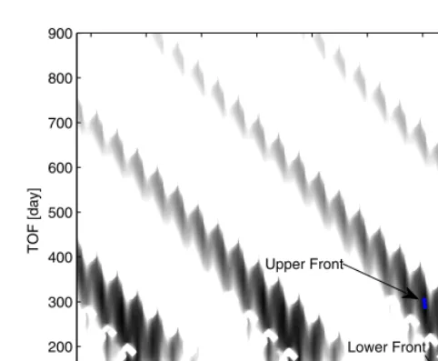
contour lines of the sum of the twoΔv is represented in Fig. 3 for t0∈[3675,10500]T
MJD2000 and T∈[50,900]days.
As can be seen in the specified solution space D there is a large number of local minima. Each minimum has a different value but some of them are nested, very close to each other with similar values. For each local minimum, there can be a different front of locally Pareto optimal solutions. The global Pareto front should contain the best transfer with minimum totalΔv and the fastest transfer with minimum TOF.
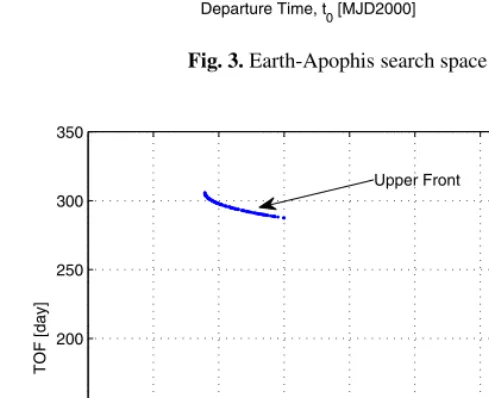
The best known approximation of the global Pareto front is represented in Fig. 4. It is a disjoint front corresponding to two basins of attraction of two minima as can be seen in Fig. 5. The lower front is made of solutions with a very low transfer time, the upper front, instead, is made of solutions with a much longer transfer time but a total Δv similar to the one of the solutions belonging to the lower front.
Departure Time, t
0 [MJD2000]
Time of Flight, T [day]
4000 5000 6000 7000 8000 9000 10000 100
200 300 400 500 600 700 800 900
[image:17.512.88.330.66.261.2]0 2 4 6 8 10 12 14 16 18 20
Fig. 3. Earth-Apophis search space
4.2 4.3 4.4 4.5 4.6 4.7 4.8 4.9 5 50
100 150 200 250 300 350
TotalΔ v [km/s]
TOF [day]
Upper Front
Lower Front
Fig. 4. Earth-Apophis transfer: dual front
[image:17.512.87.332.301.500.2]Departure Time t
0 [MJD2000]
TOF [day]
4000 5000 6000 7000 8000 9000 10000 100
200 300 400 500 600 700 800 900
5 10 15 20
Upper Front
[image:18.512.89.330.64.262.2]Lower Front
[image:18.512.103.323.321.378.2]Fig. 5. Earth-Apophis transfer: distribution of the solutions in the search space
Table 3. Comparison of the metrics M1and M2ont he Earth-Apophis case
Approach Metric 3000 6000 9000
EPIC M1 4% (39.00) 38% (22.28) 51% (17.53) M2 1.89 (5.9) 1.66 (5.14) 0.66 (3.22) NSGA-II M1 10% (26.51) 19% (27.54) 24% (25.63)
M2 20.96 (27.78) 11.99 (16.20) 10.12 (12.82)
In order to test the multi-objective optimizers with this simple but typical space tra-jectory design problem, we define two metrics:
M1=
1 Mp
Mp
∑
i=1
min j∈Np
100fj−fi fi
(21)
M2=
1 Np
Np
∑
i=1
min j∈Mp
100fj−fi fj
(22)
Although similar, the two metrics are measuring two different things: M1is the sum,
over all the elements in the global Pareto front, of the minimum distance of all the elements in the Pareto front Npfrom the the ith element in the global Pareto front. M2,
instead, is the sum, over all the elements in the Pareto front Np, of the minimum distance of the elements in the global Pareto front from the ith element in the Pareto front Np.
4 4.5 5 5.5 6 6.5 50
100 150 200 250 300 350
TotalΔ v [km/s]
TOF [day]
M
1=39.06%,M2=13.47
NSGA−II Global Pareto Front
4.3 4.4 4.5 4.6 4.7 4.8 4.9 5 50
100 150 200 250 300 350
TotalΔ v [km/s]
TOF [day]
M
1=38.96%,M2=0.64
[image:19.512.86.333.57.480.2]Global Pareto Front EPIC
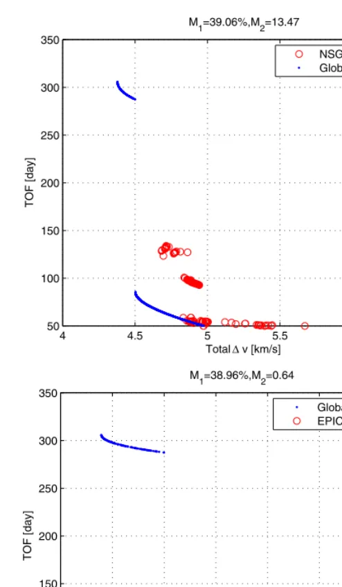
Fig. 6. Earth-Apophis transfer: comparison of two not-converged runs
a low value. If both metrics are high then the Pareto front Np is partial and poorly accurate. In Table 3 we represented metrics M1 and metrics M2, in brackets, for an
increasing number of function evaluations and for two different optimizers.
4000 5000 6000 7000 8000 9000 10000 100 200 300 400 500 600 700 800 900
Departure Date t 0 [MJD2000]
Time of Flight T [day]
Step 1
Lower part of the global front
4.5 4.6 4.7 4.8 4.9 5 50 55 60 65 70 75 80 85 90
TotalΔ v [km/s]
TOF [day]
Step 1
4000 5000 6000 7000 8000 9000 10000 100 200 300 400 500 600 700 800 900
Departure Date t 0 [MJD2000]
Time of Flight T [day]
Step 2
Lower part of the global front Local front
4.5 5 5.5 6 6.5 7 7.5 8 8.5 50 100 150 200 250 300
TotalΔ v [km/s]
TOF [day]
Step 2
Lower part of the global front Local front
4000 5000 6000 7000 8000 9000 10000 100 200 300 400 500 600 700 800 900 Step 3
Departure Date t 0 [MJD2000]
Time of Flight T [day]
Upper Part of the global front
4 4.5 5 5.5 6 6.5 7 50 100 150 200 250 300 350
TotalΔ v [km/s]
TOF [day]
Step 3
[image:20.512.65.365.60.410.2]Upper part of the global front
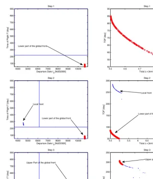
Fig. 7. Earth-Apophis transfer: domain decomposition process. The red circles are the
non-dominated solutions at each step while the blues dots are the whole set of solutions3.
performed several tests to find a good population size. The results in Table 3 were the best obtained over all the runs. For 3000 function evaluations we used a population of 200 individuals while for the 6000 evaluations and the 9000 evaluations test we used a population of 300 individuals since it was returning better results.
For each number of function evaluations we performed 100 independent runs. The table reports the percentage of times the metric M1is below 2%, and in brackets the
average value of M1 over the 100 runs. It should be noted that a value of M1 larger
than 2% up to 10% does not necessary correspond to a fully unsuccessful run. The 2% tolerance, on the other hand, guarantees that the algorithm was able to identify both parts of the Pareto front with a good distribution of the points.
In the Table 3 we also reported the average value and the standard deviation (in brackets) of metric M2. This second metric measures the accuracy of the convergence
to even a portion of the whole Pareto front.
As can be seen for a low number of function evaluations, NSGA-II performs better than EPIC, though EPIC achieves a better value of M2, which means a better local
convergence on average. Conversely, when NSGA-II is not converging to the global front, is converging to a local front, while when EPIC is not converging to the whole global front is converging to a portion of it. Figs. 6 are showing two typical cases in which the metric M1is over 30% for both the optimization algorithms. In both cases the
number of function evaluations is 3000.
Fig. 7 shows an example of the domain decomposition process. At step 1 MACS is run on the entire search space D and in this example identifies only the lower part of the global front. The search space is then partitioned in two subdomains and MACS is run on the unexplored one. The second step leads to the identification of a local front. The third step explores the unexplored subdomain and identifies the upper part of the global front. At each step MACS was run for 3000 function evaluations.
For a higher number of function evaluations, NSGA-II progressively increases the number of successes, though the accuracy remains lower than for EPIC. The large pop-ulation of NSGA-II, in fact, samples the solution space better than the small poppop-ulation of EPIC. On the other hand the decomposition of the solution space allows EPIC to increase the exploration even with a small number of agents. This is demonstrated by the number of successful runs which is more than double than the one of NSGA-II.
6
Conclusions
In this chapter we presented a hybrid behavioral-based search algorithm for multiobjec-tive optimization problems. We showed its effecmultiobjec-tiveness on a set of standard problems and in particular on a space trajectory design problem. The latter, though very simple, well illustrates some typical difficulties in the use of global methods for the design of space trajectories.
References
1. Chipperfield, A.J., Fleming, P.J., Pohlheim, H., Fonseca, C.M.: Genetic Algorithm Toolbox User’s Guide, ACSE Research Report No. 512, University of Sheffield (1994)
2. Horst, R., Tuy, H.: Global optimization: deterministic approaches, 3rd edn. Springer, Berlin (1996)
3. Stephens, C.P., Baritompa, W.: Global optimization requires global information. Journal of Optmization Theory and Applications 96, 575–588 (1998)
4. Storn, R., Price, K.: Differential Evolution – a Simple and Efficient Heuristic for Global Op-timization over Continuous Spaces. Journal of Global OpOp-timization 11(4), 341–359 (1997) 5. Torn, A., Zilinskas, A.: Global Optimization. Springer, Berlin (1987)
6. Kennedy, J., Eberhart, R.: Particle swarm optimization. In: Proceedings of the IEEE Interna-tional Conference on Neural Networks, pp. 1942–1948 (1995)
7. Perttunen, C.D., Stuckman, B.E.: Lipschitzian Optimization Without the Lipschitz Constant. JOTA 79(1), 157–181 (1993)
8. Price, K.V., Storn, R.M.: Jouni A. Lampinen. Differential Evolution: A Practical Approach to Global Optimization, 1st edn. Springer, Heidelberg (December 22, 2005)
9. Deb, K., Pratap, A., Meyarivan, T.: Fast elitist multi-objective genetic algorithm: NGA-II. KanGAL Report No. 200001 (2000)
10. Deb, K., Pratap, A., Meyarivan, T.: Constrained test problems for multi-objective evolution-ary optimization. KanGAL Report No. 200002 (2002)
11. Sierra, M.R., Coello, C.A.C.: A Study of Techniques to Improve the Efficiency of a Multi-Objective Particle Swarm Optimizer. Evolutionary Computation in Dynamic and Uncertain Environments, 269–296 (2007)
12. Coello, C.A.C., Lamont, G., Van Veldhuizen, D.: Evolutionary Algorithms for Solving Multi-Objective Problems, 2nd edn. Springer, New York (2007)
13. Gage, P.J., Braun, R.D., Kroo, I.M.: Interplanetary trajectory optimisation using a genetic algorithm. Journal of the Astronautical Sciences 43(1), 59–75 (1995)
14. Gurfil, P., Kasdin, N.J.: Niching genetic algorithms-based characterization of geocentric or-bits in the 3D elliptic restricted three-body problem. Computer Methods in Applied Mechan-ics and Engineering 191(49-50), 5673–5696 (2002)
15. Hartmann, J.W., Coverstone-Carrol, V.L., Williams, S.N.: Optimal Interplanetary Space-craft Trajectories via Pareto Genetic Algorithm. Journal of the Astronautical Sciences 46(3) (1998)
16. Rauwolf, G., Coverstone-Carroll, V.: Near-optimal low-thrust orbit transfers generated by a genetic algorithm. Journal of Spacecraft and Rockets 33(6), 859–862 (1996)
17. Vasile, M.: Combining Evolution Programs and Gradient Methods for WSB Transfer misation. In: Operational Research in Space & Air, vol. 79, Book Series in Applied Opti-mization Kluwer Academy Press (2003) ISBN 1-4020-1218-7
18. De Pascale, P., Vasile, M.: Preliminary Design of Low-Thrust Multiple Gravity Assist Tra-jectories. Journal of Spacecraft and Rockets 43(5), 1065–1076 (2006)
19. Dachwald, B.: Optimization of interplanetary solar sailcraft trajectories using evolutionary neurocontrol. Journal of Guidance, and Dynamics (January/ February 2004)
20. Myatt, D.R., Becerra, V.M., Nasuto, S.J., Bishop, J.M.: Advanced Global Optimization Tools for Mission Analysis and Design. Final Rept. ESA Ariadna ITT AO4532/18138/04/NL/MV, Call03/4101 (2004)
22. Dam, R.E., van Husslage, B.G.M., den Hertog, D., Melissen, J.B.M.: Maximin Latin hyper-cube designs in two dimensions. Operations Research 55, 158–169 (2007)
23. Battin, R.H.: An Introduction to the Mathematics and Methods of Astrodynamics, Revised Edition (Aiaa Education Series). AIAA (American Institute of Aeronautics & Ast; Revised edition (1999) ISBN-13: 978-1563473425
24. Vasile, M.: A Behavioral-based Meta-heuristic for Robust Global Trajectory Optimization. In: IEEE Congress on Evolutionary Computing (CEC 2007) Proceedings, pp. 2056–2063 (2007)