Fitting a geometric graph to a protein-protein interaction network

Fitting a geometric graph to a protein–protein interaction network

Desmond J. Higham

, Marija Rasˇajski

and Natasˇa Przˇulj

*

1

Department of Mathematics, University of Strathclyde, Glasgow G1 1XH, UK,2Department of Computer Science, UC Irvine, Irvine, CA 92697, USA and3Faculty of Electrical Engineering, University of Belgrade, Belgrade, Serbia

Received on September 19, 2007; revised on February 8, 2008; accepted on February 27, 2008

Advance Access publication March 14, 2008

Associate Editor: Olga Troyanskaya

ABSTRACT

Motivation:Finding a good network null model for protein–protein interaction (PPI) networks is a fundamental issue. Such a model would provide insights into the interplay between network structure and biological function as well as into evolution. Also, network (graph) models are used to guide biological experiments and discover new biological features. It has been proposed that geometric random graphs are a good model for PPI networks. In a geometric random graph, nodes correspond to uniformly randomly distributed points in a metric space and edges (links) exist between pairs of nodes for which the corresponding points in the metric space are close enough according to some distance norm. Computational experiments have revealed close matches between key topological properties of PPI networks and geometric random graph models. In this work, we push the comparison further by exploiting the fact that the geometric property can be tested for directly. To this end, we develop an algorithm that takes PPI interaction data and embeds proteins into a low-dimensional Euclidean space, under the premise that connectivity information corresponds to Euclidean proximity, as in geometric-random graphs. We judge the sensitivity and specificity of the fit by computing the area under theReceiver Operator Characteristic(ROC) curve. The network embedding algorithm is based on multi-dimensional scaling, with the square root of the path length in a network playing the role of the Euclidean distance in the Euclidean space. The algorithm exploits sparsity for computational efficiency, and requires only a few sparse matrix multiplications, giving a complexity ofO(N2_{) where}

Nis the number of proteins.

Results: The algorithm has been verified in the sense that it successfully rediscovers the geometric structure in artificially con-structed geometric networks, even when noise is added by re-wiring some links. Applying the algorithm to 19 publicly available PPI networks of various organisms indicated that: (a) geometric effects are present and (b) two-dimensional Euclidean space is generally as effective as higher dimensional Euclidean space for explaining the connectivity. Testing on a high-confidence yeast data set produced a very strong indication of geometric structure (area under the ROC curve of 0.89), with this network being essentially indistinguishable from a noisy geometric network. Overall, the results add support to the hypothesis that PPI networks have a geometric structure.

Availability:MATLAB code implementing the algorithm is available upon request.

Contact:[email protected]

1 INTRODUCTION

Large, complex networks (also called graphs) arise in a vast array of applications (Newman, 2003). Efforts to develop models that describe and summarize complex networks have focused on various network features such as motifs (Miloet al., 2002), graphlets (Przˇulj et al., 2004) and graphlet degree distributions Przˇulj (2006), clustering coefficients (Watts and Strogatz, 1998), pathlengths (Watts and Strogatz, 1998) and degree distributions (Khanin and Wit, 2006; Newman, 2003; Thomaset al., 2003).

Studying protein–protein interaction (PPI) networks has recently become possible due to advances in experimental high-throughput technologies such as yeast-2-hybrid (Y2H) (Y2H) (Ito et al., 2000; Uetz et al., 2000), tandem affinity purification (TAP) (Gavin et al., 2002) and high-throughput mass spectrometric protein complex identification (HMS-PCI) (Ho et al., 2002). A significant amount of experimental PPI network data for several organisms has already been generated. (Gavinet al., 2002; Giotet al., 2003; Hoet al., 2002; Itoet al., 2000; Krogan et al., 2006; Li et al., 2004; Rual et al., 2005; Stelzlet al., 2005; Uetzet al., 2000).

Understanding the patterns of intricate wiring in PPI networks is clearly of great importance for basic biological understanding, and also has the potential to feed back into the strategies for optimal interactome detection (Lappe and Holm, 2004). Further benefits of an accurate PPI model include (a) generation of synthetic datasets of any size in order to test computational algorithms, (b) detection of false positives and false negatives, (c) possible insights into the evolutionary processes that created the network and (d) convenience of representing complex networks in terms of a small number of model parameters and thereby distinguishing between networks for different organisms. Thus, modelling of PPI networks has become an active research area and several different random graph models have already been suggested (Grindrod, 2002; Grindrod and Kibble, 2004; Morrisonet al., 2006; Przˇulj and Higham, 2006; Przˇuljet al., 2004; Thomaset al., 2003; Vazquez

et al., 2001). Among them aregeometric random graphs(Przˇulj

et al., 2004, 2006) in which nodes correspond to uniformly randomly distributed points in a low-dimensional Euclidean space and edges exist between pairs of nodes in the graph if the corresponding points in the space are close enough (within some radius ) according to the Euclidean distance

norm. Other models include: Erdo¨s–Re´nyi random graphs

1998),scale-free(Baraba´si and Albert, 1999; Simon, 1955) and

stickiness(Przˇulj and Higham, 2006) networks.

Our research focuses on geometric random graphs. The key observation that drives our work is that, in contrast with other putative PPI models, the geometric structure can be examined constructively. To test whether a given PPI network has a geometric structure, rather than measuring local and global statistics of the PPI network and comparing these with local and global statistics of random geometric graphs, a more direct question can be addressed:

Can we represent the given PPI network as a geometric graph by embedding the proteins in R2, R3 or R4 and finding ansuch that proteins are connected if and only if

they are-close?

There are two main themes to this work. The first theme is designing and testing an algorithm to discover whether a network has an underlying geometric structure. This theme is dealt with in Sections 2–4. The second theme, covered in Section 5, is to use this tool to study PPI networks.

We remark that the reverse engineering problem considered here is related to the general, but less well-defined, tasks of ordering and clustering (Grindrod, 2002; Grindrod and Kibble, 2004; Titzet al., 2004). Spectral (eigenvalue/eigenvector-based) algorithms have proved successful for ordering and clustering (Grindrod and Kibble, 2004; Higham, 2003), and this provides motivation for a spectral algorithm to address the geometric embedding issue.

2 THEORETICAL BASIS

As in previous studies (Przˇulj, 2006; Przˇulj et al., 2004), we focus on non-periodic, uniform, Euclidean geometric random graphs in R2_,

R3 _and

R4_{. These are defined as follows [see}

Penrose (2003) for further details about geometric random graphs and their properties]. In the two-dimensional (2D) case, to create a network (an undirected, unweighted graph) withN

nodes we place a set ofNpoints,fx½i_gN

i¼1, uniformly in the unit

square; that is, each x[i]₂R2 has its two components drawn independently from the uniform (0,1) distribution, and all points are generated independently. Then, for each pair of points (x[i]_,x[j]_{), we create an edge between nodesiandjof the}

geometric random graph if and only ifIx[i]x[j]I2, whereII2

denotes Euclidean distance and4_{0 is a parameter. In other}

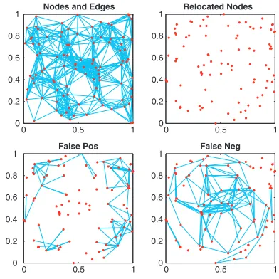
words, nodesiandjare linked if and only if pointsiandjare within Euclidean distance . The process is illustrated in the

upper left picture of Figure 1. The three-dimensional (3D) and four-dimensional (4D) cases are defined analogously, by placing points inR3andR4.

Our algorithm makes use of ideas from multi-dimensional scaling (MDS). We summarize here the necessary details, referring the reader to (Cox and Cox, 1994) for further information and historical references, and (Kaskiet al., 2003; Taguchi and Oono, 2004) for examples where MDS has been used in bioinformatics.

Suppose that, for a set ofNobjects, we are given thepairwise Euclidean distances dij between all pairs, and we are asked to find a set ofNvectorsfx½i_gN

i¼1inR

m

such that

kx½i_x½j_k2¼d

ij; for alli,j: ð1Þ

In other words, our task is to find locations in Rm for the objects so that the pairwise distances are respected. Finding the smallest dimension m for which a solution is possible may be regarded as part of the problem. In our context, we will think of the dimension as being fixed at 2, 3 or 4, and we will be seeking N locations fx½i_gN

i¼1 for which the

constraints (1) are well approximated in a sense that will be made precise.

Given data {dij} that respects the triangle inequality,double centeringproduces the symmetric, positive semi-definite matrix

A₂RNN_{defined by}

aij¼ 12 d 2

ij1n

Xn

k¼1 d2_ik1

n

Xn

k¼1 d2_kjþ1

n2 Xn

k¼1 Xn

l¼1 d2_kl

!

: ð2Þ

LettingX₂RmNbe the matrix whosejth column isx[j], it may then be shown that

XTX_¼A _{) k}x½ix½j_k2¼dij; for alli,j: ð3Þ

Now A has the real Schur decomposition (Golub and Van Loan, 1996) A_¼UTU, where U₂RNN is orthogonal (its rows are eigenvectors ofA) and_¼diag(i) is diagonal with diagonal entries ordered high-to-low (these are the eigenvalues ofA). We then see that a solutionX in (3) may be computed as

X_¼12_U: ð4Þ

0 0.5 1

0 0.2 0.4 0.6 0.8

0 0.5 1

0 0.2 0.4 0.6 0.8

0 1

0 0.2 0.4 0.6 0.8

1 False Pos

0 1

0 0.2 0.4 0.6 0.8

1 False Neg

0.5 0.5

To find an ‘optimal’ approximation such that x[i]₂Rr, we may truncate (4) using only thermost positive eigenvalues, so that

b X_¼

ffiffiffiffiffi 1

p _u½1T _{. . . . . .}

. . .

ffiffiffiffiffi r

p _u½rT . . . . 2

6 6 4

3 7 7

5; ð5Þ

whereu[k]₂RNis thekth row ofU. This is optimal in the sense thatXbis the closest rank-r matrix to X, in any orthogonally invariant norm (Golub and Van Loan, 1996).

3 INITIAL ALGORITHM

In this section, we outline the main ideas behind the algorithm and show how we propose to evaluate its accuracy. Our task is to embed proteins intoR2, R3or R4given the PPI network. Rather than Euclidean distances, we have only {0,1} connect-ivityinformation. For this reason, we will use a function of the pathlength in lieu of Euclidean distance. By construction, if nodes A and B in a geometric graph are connected (pathlength one), then their Euclidean distance is between zero and .

Similarly, a pathlength of two indicates that an intermediate node, C, is-close to both A and B, with the Euclidean distance

between A and B lying somewhere between and 2. In the

absence of exact distance information we will adopt the heuristic that a ‘typical’ configuration has a right angle for the angle ABC, and assume that a typical length-two path corresponds to a distance ofpffiffiffi2. The square root can also be

regarded as an attempt to compromise between the opposing factors where (1) one of the distances A-to-C or C-to-B is much less thanand (2) the nodes A, B and C are co-linear. More

generally, we will use the square root of the graph pathlength in lieu of Euclidean distance, so that_{ffiffiffiffiffiffiffiffiffiffiffiffi} dij in (1) is taken to be

pathij

p

, where pathij denotes the pathlength between nodes iandj. In practice, we tried several alternative monotonically increasing functions of pathij and found that the resulting algorithm was insensitive to this detail.

A minor issue is the natural scale-invariance of the problem—re-scaling and the distances dij does not change the network. Because the traditional geometric model assumes that all points lie in the unit disk/cube, we will normalize the coordinate vectors in (5) so that

ffiffiffiffiffi _k p

u½_jk° ffiffiffiffiffi _k p _u½k

j mini pffiffiffiffiffi_ku½_ik

maxi pffiffiffiffiffi_ku½_ik

mini pffiffiffiffiffi_ku½_ik

: ð6Þ

We now illustrate these ideas on data arising from a small geometric graph in R2 for which the results can be easily visualized. Here we tookN_¼100 nodes with coordinates drawn independently from the uniform (0, 1) distribution and joined nodes that were within Euclidean distance ¼0.25. The

resulting graph is shown in the upper left picture of Figure 1. The six most positive eigenvalues ofAin (2), using ffiffiffiffiffiffiffiffiffiffiffiffipathij

p

for

dij, were found to be 39.9, 31.3, 8.7, 7.4, 6.1 and 4.0. If we had used exact Euclidean distance information then, since we started with a geometric graph inR2, it would be possible to embed exactly in R2, so that only the first two eigenvalues

would be non-zero. In using pathlength to approximate Euclidean distance, we have lost this property, but it is reassuring that the first two eigenvalues remain strongly dominant. The 2D embedding from the algorithm is shown in the upper right, and the lower pictures display the false positives and false negatives arising when a geometric graph with radius¼0.25 is formed.

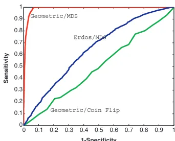
To measure the ability of the algorithm to recover the original network, we present a receiver operator characteristic (ROC) curve (Bradley, 1997; Tape, 2000) in Figure 2, marked

Geometric/MDS. Here, we increasedfrom 0 topffiffiffi2in small

increments, and for each we generated the geometric graph

arising from the MDS node placement as in the upper right picture of Figure 1. The horizontal axis is then defined as 1specificity, that is, 1TN/(TNþFP), and the vertical axis is defined as sensitivity, that is TP/(TPþFN). Here TN denotes the number of true negatives that is, the number of distinct pairs

iandjfor which there is no edge in the reverse engineered graph

andthere is no edge in the original graph. Similarly, TP, FP and FN denote the number of true positives, false positives and false negatives, respectively. With ¼0, we place no edges in the

network, and hence we have perfect specificity, 1TN/ (TNþFP)¼0, but the worst possible sensitivity, TP/ (TPþFN)¼0. The other extreme ¼pffiffiffi2connects all nodes,

giving the worst possible specificity, 1TN/(TNþFP)¼1, but perfect sensitivity, TP/(TP_þFN)_¼1. Increasing always

improves sensitivity at the expense of specificity. Good performance corresponds to having a curve that rises rapidly, containing points close tox_¼0,y_¼1, and the area under the curve (AUC) is a widely-used measure of quality (Bradley, 1997; Tape, 2000). In Figure 2 we have an AUC of 0.988 for MDS curve.

For comparison, we have added two more ROC curves in Figure 2. First, for the same network, we show the effect of ‘randomly guessing’ links. Here, we take a biased coin that lands heads with probabilityp. For each pair of nodes we flip the coin and predict a link if the coin lands heads. Aspis varied this leads to the ROC curve labelledGeometric/Coin Flip, which has an AUC of 0.47. Next, we generated a network with

0 0.1 0.2 0.3 0.4 0.5 0.6 0.7 0.8 0.9 1

0 0.1 0.2 0.3 0.4 0.5 0.6 0.7 0.8 0.9 1

Sensitivity

1-Specificity Geometric/MDS

Geometric/Coin Flip Erdos/MDS

Fig. 2.ROC curves displaying sensitivity and specificity. Upper curve, markedGeometric/MDS, arises from our MDS-based algorithm on a geometric network. Lower curve, marked Geometric/Coin Flip, arises when interactions are predicted at random for the geometric network. Middle curve, markedErdos/MDS, arises when our MDS-based algorithm is applied to an Erdo¨s-Re´nyi random graph.

95

Instead we used an Erdo¨s–Re´nyi model (Erdo¨s and Re´nyi, 1959, 1960) as in (Przˇuljet al., 2004) where, for each pair of nodes, a link was inserted with independent probability 0.8. Applying our MDS-based algorithm produced the ROC curve labelledErdos/MDS, which has an AUC of 0.64.

4 PRACTICAL ALGORITHM

For PPI networks, where the number of nodes is typically in the thousands, we propose setting

dij¼

ffiffiffiffiffiffiffiffiffiffiffiffi

pathij

p

; if path_ijK; Kmax; otherwise: (

ð7Þ

whereKand Kmax are parameters in the algorithm. Here we

have introduced a cutoffK with longer pathlengths rounded to a single valueKmax. Using the cutoff Kin (7), rather than

computing and recording the pathlength for all pairs, has three main advantages.

(1) By choosing K relatively small, the resulting algorithm can exploit sparsity in the original network. This is explained further below.

(2) The case where the network consists of two or more disconnected components (i.e. some pathlengths are infinite) is conveniently handled.

(3) The cutoff reflects the fact that for a true geometric graph in the unit cube, there is an upper bound on the maximum Euclidean distance.

We remark that, intuitively, it is clear that accurate information concerning near-neighbours is more important than informa-tion concerning distant nodes. In our experiments, we found that the results from the algorithm were not sensitive to the choice of K and Kmax, although, as explained below, the

computational benefits can be dramatic.

Repeating the experiment in Figure 1, but with parameters

K_¼4 andKmax¼5, gave rise to leading eigenvalues 38.3, 30.1,

10.7, 8.9, 6.2 and 3.8, and an area under the ROC curve of 0.984, showing that retaining level-four path information is adequate in this case. Similar effects were observed more generally, so we used these values in all computations.

We now explain how our distance measure (7) allows sparsity to be exploited. To measure complexity, we assume that the number of connections per protein is fixed, independently ofN, and we consider asymptotics as N_{! 1}. We assume that subspace iteration (Golub and Van Loan, 1996) is used to compute eigenpairs of the matrix A in (2). The significant computational task is then the formulation of a matrix-vector product; given some v₂RN compute the product Av. By construction the elementsd2

ijin (2) now come from a matrix of

the formP_þKmax11T, where12RNdenotes the vector of 1’s,

and hence11T2RNNis the matrix of 1’s, andPhas values

pij¼

ffiffiffiffiffiffiffiffiffiffiffiffi

pathij

p

Kmax; if path_ijK;

0; otherwise. (

ð8Þ

Hence,pijis non-zero only when there is a path of lengthK between proteins i and j. In other words, P has the same

the network. For a fixed value ofK, this means thatPhas the same sparsity as the original network. It then follows that the productAvmay be written

Av_¼ 1

2 Pv hvipsumþ

Nhvi vT_p

N

1

; ð9Þ

where psum2R

N

has ðp_sumÞi¼PN_j¼1pij, hvi 2R denotes the

average valuevT1/Nand2RdenotesPN_i¼1PN_j¼1p_ij.

It follows that each step of the subspace iteration involves a matrix–vector multiply with a sparse matrix. In our computa-tions, we stopped the iteration when successive eigenvector approximations agreed to within 103_{in Euclidean norm.}

Overall, given a protein–protein interaction network, our algorithm may be summarized as:

(1) Compute the pathlengths up to lengthK.

(2) Compute the first two, three or four most positive eigenvalues ofA, and the corresponding eigenvectors. (3) Embed the nodes inR2,R3orR4using (5) and (6). (4) Examine the accuracy of the embedding asis varied.

To measure computational cost we note that a sparse matrix– vector multiplyAvis anO(N) process. Step 1 of the algorithm can be achieved by forming the matrices A, A2_{, A}3_{,. . .,A}K_, which has, at most, an O(N2) operation count. Step 2 costs

O(N) per iteration of the subspace iteration algorithm. Step 3 is negligible. In Step 4, having generated the protein locations, computing the pairwise distance data {kx[i]x[j]_k2}i6¼j, so that choices forcan be tested, is anO(N2) task.

5 DATA AND RESULTS

5.1 PPI networks

Using high-throughput techniques such as Y2H (Ito et al., 2000; Uetzet al., 2000), TAP (Gavinet al., 2002) and HMS-PCI (Hoet al., 2002), a significant amount of experimental PPI data has been generated. Our algorithm has been applied to 19 PPI networks of four eucaryotic organisms: yeast Saccharomyces cerevisiae, fruitfly Drosophila melanogaster, nematode worm

Caenorhabditis elegans and human. We used nine yeast, one fruitfly, three worm and six human PPI networks obtained from different studies that used different PPI detection techniques, as well as from curated databases (described below).

The high-confidence part of the yeast PPI network described by (von Meringet al., 2002) is henceforth denoted by ‘YHC’. This dataset is discussed in more detail in the next subsection. We denote by ‘Y11K’ the yeast PPI network defined by the top 11 000 interactions in the (von Meringet al., 2002) classifica-tion. ‘YIC’ denotes the ‘core’ yeast PPI network from (Itoet al., 2000) Y2H study. We denote by ‘YIP’ the entire yeast PPI network from (Ito et al., 2000). ‘YU’ stands for yeast PPI network from (Itoet al., 2000). Y2H study. ‘YICU’ is the union of yeast PPI networks from Ito et al. (2000) and Uetz et al.

obtained by TAP and matrix-assisted laser desorption/ioniza-tion-time of flight mass spectrometry and liquid chromatogra-phy tandem mass spectrometry. ‘YM’ is the yeast PPI network from MIPS (Meweset al., 2002). ‘FH’ is the high-confidence part of the fruitfly PPI network from (Giot et al., 2003) in which a two-hybrid-based protein-interaction map of the fly proteome has been presented.

‘WE’ is the entire worm PPI network published by Liet al., (2004), where more than 4000 interactions were identified from Y2H screens, and ‘WC’ denotes the ‘core’ part of the worm PPI network also from (Li et al., 2004). By ‘WS’ we denote the worm PPI network from (Zhong and Sternberg, 2006), where prediction techniques have been used to generate this PPI network, consisting of 18 183 interactions.

The human PPI network from (Stelzlet al., 2005), obtained by Y2H screens, which contains high- medium- and low-confidence data is denoted by ‘HSL’, its part that contains only and medium-confidence data ‘HSM’, and only high-confidence interaction from this study by ‘HSH’. ‘HR’ is the human PPI network from (Rualet al., 2005), also obtained by Y2H screens. By ‘HH’ we denote the human PPI network from the human protein reference database (HPRD) (Peri et al., 2004). We denote by ‘HM’ the human PPI network from MINT (Zanzoniet al., 2002).

5.2 Results

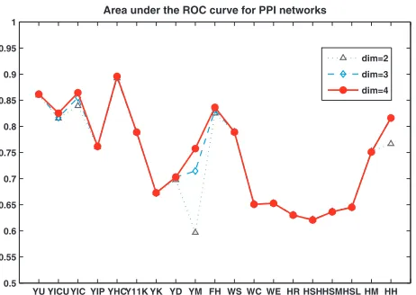
Using the algorithm described in section 4, we embedded these networks in 2D, 3D and 4D space. The resulting areas under the ROC curves are shown in Figure 3. One striking feature is that using only two dimensions typically gives results that are as good as the cases where dimension three or four is used. Of the 19 PPI networks, all but the YM 2D case produce an area under the ROC curve >0.6, and 11 networks have areas under the ROC curves above 0.75. Note that some of the human PPI networks (Rualet al., 2005; Stelzlet al., 2005) that we analysed come from the first Y2H studies of the human interactome and thus are considered to be of low confidence (‘HR’, ‘HSL’, ‘HSM’, and ‘HSH’ in Figure 3). We expect that low areas under the ROC curve for these networks are due to the noise present in them. Human PPI networks from curated databases MINT and HPRD are of higher confidence than the PPI networks from Y2H studies resulting in high areas under the ROC curve (see ‘HM’ and ‘HH’ in Figure 3).

5.3 Further tests

5.3.1 High-confidence data YeastS.Cerevisiae is an organ-ism important for research in human biology. Von Mering

et al., (2002) performed a systematic synthesis and evaluation of PPIs obtained using the main high-throughput PPI detection methods for yeast. They integrated 78 390 interactions between 5321 yeast proteins, out of which 2455 are identified by more than one PPI detection method (von Meringet al., 2002). This high-confidence PPI network, which has 2455 interactions amongst 988 proteins, appears as YHC in Figure 3. The actual areas under the ROC curve are 0.892, 0.893, 0.896 for embedding into 2D, 3D and 4D space, respectively. This represents a very good match to the geometric model and,

reassuringly, it is the best over all the datasets. Hence, in our further investigations we will focus on this YHC data.

5.3.2 Geometric structure in other random network models Modelling real-world networks by various types of random graphs began with the work of Erdo¨s and Re´nyi. One classical random graph model connects nodes uniformly at random with some fixed probability (Erdo¨s and Re´nyi, 1959, 1960). This simple model does not describe many important properties of real-world networks such as degree distribution and clustering coefficients. Efforts to improve the applicability of these networks producedgeneralized random graphs(Bender and Canfield, 1978) in which the edges are chosen at random as in Erdo¨s–Re´nyi graphs, but the degree distribution matches the degree distribution of the real network. Attempts to further improve global properties of the real-world networks led to numerous types of models such as small-world (Watts and Strogatz, 1998) and scale-free (Baraba´si and Albert, 1999; Simon, 1955) networks. Other models have been constructed with the idea of simulating some biological and topological properties of real biological networks, e.g. stickiness model (Przˇulj and Higham, 2006).

In Figure 4 we present the results of an experiment to measure the extent to which several random graph models can produce a geometric structure. Here, seven types of random networks have been generated corresponding to, i.e. having the same number of nodes and edges as, the dataset YHC: Erdo¨s– Re´nyi random graphs (denoted by ‘ER’), random graphs with the same degree distribution as the data (denoted by ‘ER-DD’), 2D geometric random graphs (‘GEO-2D’), 3D geometric random graphs (‘GEO-3D’), 4D geometric random graphs (‘GEO-4D’), scale-free Barabasi–Albert model graphs (‘SF’) and stickiness model graphs (‘STICKY’). Note that ‘ER-DD’, ‘SF’, and ‘STICKY’ are three different types of scale-free networks. For each type, 30 networks have been generated, embedded in 2D, 3D and 4D space, and the area under the ROC curve has been computed. Results are also shown for networks obtained from randomly rewiring 10% (‘G-10P’), 20% (‘G-20P’), and 30% (‘G-30P’) of edges in a 3D geometric

YU YICU YIC YIP YHCY11K YK YD YM FH WS WC WE HR HSHHSMHSL HM HH 0.5

0.55 0.6 0.65 0.7 0.75 0.8 0.85 0.9 0.95 1

Area under the ROC curve for PPI networks

dim=2

dim=3

dim=4

Fig. 3. Values of the areas under the ROC curve arising from embedding nine yeast, one fruitfly, three worm, and six human PPI networks into 2D, 3D and 4D Euclidean space.

random graph, in an attempt to account for false positives and false negatives (further details in Section 5.3.3). The mean and the SD for AUC of these networks are shown in Figure 4, and we see that the algorithm clearly distinguishes between geometric and non-geometric models including scale-free net-works. In other words, even allowing for noise in the data, the lack of geometric structure in the other models is apparent.

5.3.3 Robustness of our approach Unfortunately, noise is inherent in all current PPI networks (Mrowkaet al., 2001). On one hand, PPI datasets contain a large percentage of false positive interactions. One example is when proteins interact indirectly, i.e. through mediation of one or more molecules, but this is recorded as a direct physical interaction by the experimental method. On the other hand, imperfect experi-mental methods lead to false negative interactions. Different biochemical techniques produce different sets of false positives and negatives. Thus, trying to find high-confidence PPI networks by overlapping multiple datasets may result in dis-carding many real interactions.

Since the PPI networks are thought to contain a large percentage of false negatives and a large percentage of false positives, we tested with simulated noise. From Figure 4, we see that for randomly generated GEO-3D graphs the embedding into 3D space is excellent. At the right in Figure 4 we show the effect of rewiring 10%, 20% and 30% of the edges in these GEO-3D graphs. The resulting networks are denoted by G-10P, G-20P and G-30P, respectively. We generated 30 networks of each type (corresponding to the percentages of rewired edges), embedded them in 2D, 3D and 4D space, and computed the areas under the ROC curve. The mean area under the ROC curve for the 10% rewired GEO-3D networks are: 0.811, 0.875 and 0.918, corresponding to 2D, 3D and 4D embeddings, respectively.

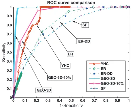
In Figure 5, ROC curves corresponding to embeddings into 3D Euclidean space of the high-confidence yeast PPI network (denoted by YHC) and the model networks ER, ER-DD, GEO-3D and SF generated with the same number of nodes and

edges as the YHC network, are presented in the same graph for comparison. Also, we included one GEO-3D network with 10% rewired edges (denoted by GEO-3D-10%). We see low areas under ROC curves for random (ER) and scale-free (ER-DD and SF) network types. We also see that the YHC– ROC curve is consistent with that of a noisy geometric network. So, overall, from the ROC curve perspective, any departure from geometric structure in the PPI network can be explained by the inherent noise.

6 DISCUSSION

It has already been established that the random geometric graph model gives an excellent fit for various global and local measures of PPI networks such as pathlengths, clustering coefficients, relative graphlet frequencies (Przˇuljet al., 2004), and graphlet degree distributions (Przˇulj, 2006). The main idea of this work is to test directly whether PPI networks are geometric by embedding them into a low-dimensional Euclidean space. We developed an algorithm that takes PPI network data and attempts to recover the geometric network structure, using specificity and sensitivity measures to quantify the results. The algorithm was demonstrated to work well on artificially constructed geometric random networks, even in the presence of noise. We applied the algorithm to the 19 PPI networks of various organisms (yeast, fruitfly, worm and human) and seven types of random network models including three types of scale-free networks. Also, we compared these results with the results of rewired geometric networks, where rewiring simulates the noise that is present in the real PPI network data. The results we obtained in this work yield support to the hypothesis that the structure of PPI networks is consistent with the structure of a noisy geometric random graph. The fact that the algorithm produced a better fit on high-confidence PPI data suggests that the algorithm could be

ER ER_DD SF STICKY GEO2D GEO3D GEO4D G-10P G-20P G-30P 0.5

0.55 0.6 0.65 0.7 0.75 0.8 0.85 0.9 0.95

dim=2 dim=3 dim=4

Fig. 4. Means and SDs of the areas under the ROC curve arising from embedding seven types of random networks and three types of rewired geometric random networks (which are used to simulate the noise present in the real data) into 2D, 3D and 4D Euclidean space.

0 0.1 0.2 0.3 0.4 0.5 0.6 0.7 0.8 0.9 1

0 0.1 0.2 0.3 0.4 0.5 0.6 0.7 0.8 0.9

Sensitivity

1-Specificity

YHC ER ER-DD GEO-3D GEO-3D-10% SF SF

ER-DD

ER

YHC

GEO-3D-10%

GEO-3D

used to help discover false positives and false negatives in PPI networks.

ACKNOWLEDGEMENTS

We thank the Institute for Genomics and Bioinformatics (IGB) at UC Irvine for providing computing resources. This project was supported by the NSF CAREER IIS-0644424 grant. M.R. is grateful to the Serbian Ministry of Science for financial support. D.J.H. was supported by grant EP/E0493701/1 from the Engineering and Physical Sciences Research Council of the UK.

Conflict of Interest: none declared.

REFERENCES

Baraba´si,A.-L. and Albert,R. (1999) Emergence of scaling in random networks.

Science,286, 509–512.

Bender,E.A. and Canfield,E.R. (1978) The asymptotic number of labeled graphs with given degree sequences.J. Combinatorial Theory A,24, 296–307. Bradley,A.P. (1997) The use of the area under the ROC curve in the evaluation of

machine learning algorithms.Pattern Recogn.,30, 1145–1159.

Cox,T.F. and Cox,M.A.A. (1994)Multidimensional Scaling. Chapman and Hall, London.

Erdo¨s,P. and Re´nyi,A. (1959) On random graphs.Publ. Math.,6, 290–297. Erdo¨s,P. and Re´nyi,A. (1960) On the evolution of random graphs.Publ. Math.

Inst. Hung. Acad. Sci.,5, 17–61.

Gavin,A.C.et al. (2002) Functional organization of the yeast proteome by systematic analysis of protein complexes.Nature,415, 141–147.

Giot,L. et al. (2003) A protein interaction map of drosophila melanogaster.

Science,302, 1727–1736.

Golub,G.H. and Van Loan,C.F. (1996)Matrix Computations. 3rd edition. Johns Hopkins University Press, Baltimore.

Grindrod,P. (2002) Range-dependent random graphs and their application to modeling large small-world proteome datasets.Phys. Rev. E,66, 066702. Grindrod,P. and Kibble,M. (2004) Review of uses of network and graph theory

concepts within proteomics.Expert Rev. Proteomics,1, 229–238.

Higham,D.J. (2003) Unravelling small world networks.J. Comp. Appl. Math.,

158, 61–74.

Ho,Y.et al. (2002) Systematic identification of protein complexes in sacchar-omyces cerevisiae by mass spectrometry.Nature,415, 180–183.

Ito,T.et al. (2000) Toward a protein–protein interaction map of the budding yeast: a comprehensive system to examine two-hybrid interactions in all possible combinations between the yeast proteins.Proc. Natl Acad. Sci. USA,

97, 1143–1147.

Kaski,S.et al. (2003) Trustworthiness and metrics in visualizing similarity of gene expression.BMC Bioinformatics,4, 48.

Khanin,R. and Wit,E. (2006) How scale-free are gene networks?J. Computat. Biol.,13, 810–818.

Krogan,N.J.et al. (2006) Global landscape of protein complexes in the yeast saccharomyces cerevisiae.Nature,440, 637–643.

Lappe,M. and Holm,L. (2004) Unraveling protein interaction networks with near-optimal efficiency.Nat. Biotechnol.,22, 98–103.

Li,S.et al. (2004) A map of the interactome network of the metazoan c elegans.

Science,303, 540–543.

Mewes,H.W.et al. (2002) MIPS: a database for genomes and protein sequences.

Nucleic Acids Res.,30, 31–34.

Milo,R. et al. (2002) Network motifs: simple building blocks of complex networks.Science,298, 824–827.

Morrison,J.L.et al. (2006) A lock-and-key model for protein–protein interac-tions.Bioinformatics,22, 2012–2019.

Mrowka,R.et al. (2001) Is there a bias in proteome research?Genome Res.,11, 1971–1973.

Newman,M.E.J. (2003) The structure and function of complex networks.SIAM Rev.,45, 167–256.

Penrose,M. (2003)Geometric Random Graphs. Oxford University Press, Oxford. Peri,S.et al. (2004) Human protein reference database as a discovery resource for proteomics.Nucleic Acids Res.,32 Database issue, D497–D501, 1362–4962 (Journal Article).

Przˇulj,N. (2006) Biological network comparison using graphlet degree distribu-tion.Bioinformatics,23, e177–e183.

Przˇulj,N. and Higham,D. (2006) Modelling protein–protein interaction networks via a stickiness index.J. R. Soc. Interface,3, 711–716.

Przˇulj,N. et al. (2004) Modeling interactome: Scale-free or geometric?

Bioinformatics,20, 3508–3515.

Przˇulj,N.et al. (2006) Efficient estimation of graphlet frequency distributions in protein–protein interaction networks.Bioinformatics,22, 974–980. Rual,J.-F.et al. (2005) Towards a proteome-scale map of the human protein–

protein interaction network.Nature,437, 1173–1178.

Simon,H.A. (1955) On a class of skew distribution functions.Biometrika,42, 425–440.

Stelzl,U.et al. (2005) A human proteinprotein interaction network: a resource for annotating the proteome.Cell,122, 957–968.

Taguchi,Y. and Oono,Y. (2004) Relational patterns of gene expression via nonmetric multidimensional scaling analysis. Bioinformatics, Advance Access, published online on October 27, 2004, doi:10.1093/bioinformatics/ bti067.

Tape,T.G. (2000) Interpreting diagnostic tests.University of Nebraska Medical Center, Available at http://gim.unmc.edu/dxtests/.

Thomas,A.et al. (2003) On the structure of protein–protein interaction networks.

Biochem. Soc. Trans.,31, 1491–1496.

Titz,B.et al. (2004) What do we learn from high-throughput protein interaction data.Expert Rev. Proteomics,1, 111–121.

Uetz,P.et al. (2000) A comprehensive analysis of protein–protein interactions in saccharomyces cerevisiae.Nature,403, 623–627.

Vazquez,A.et al. (2001) Modeling of protein interaction networks.ComPlexUs,

1, 38–44.

von Mering,C.et al. (2002) Comparative assessment of large-scale data sets of protein–protein interactions.Nature,417, 399–403.

Watts,D.J. and Strogatz,S.H. (1998) Collective dynamics of ‘small-world’ networks.Nature,393, 440–442.

Xenarios,I.et al. (2000) DIP: the Database of Interacting Proteins.Nucleic Acids Res.,28, 289–291.

Zanzoni,A.et al. (2002) Mint: a molecular interaction database.FEBS Letters,

513, 135–140.

Zhong,W. and Sternberg,P. (2006) Genome-wide prediction ofC. elegans genetic interactions.Science,311, 1481–1484.

1099