Global trajectory optimisation: can we prune the solution space when considering deep space manoeuvres?

(1)

Vasile, M. and Ceriotti, M. and Radice, G. and Becerra, V.M. and Nasuto, S.J. and Anderson, J.D. Global trajectory optimisation: can we prune the solution space when considering deep space manoeuvres? [Report]

http://strathprints.strath.ac.uk/20169/

Strathprints is designed to allow users to access the research output of the University of Strathclyde. Copyright © and Moral Rights for the papers on this site are retained by the individual authors and/or other copyright owners. You may not engage in further distribution of the material for any profitmaking activities or any commercial gain. You may freely distribute both the url (http://strathprints.strath.ac.uk) and the content of this paper for research or study, educational, or not-for-profit purposes without prior permission or charge. You may freely distribute the url

(http://strathprints.strath.ac.uk) of the Strathprints website.

(2)

Global Trajectory Optimisation:

Can we Prune the Solution Space

when Considering Deep Space

Manoeuvres?

Final Report

Authors: Massimiliano Vasile, Matteo Ceriotti, Gianmarco Radice

Affiliation: Department of Aerospace Engineering, University of Glasgow, UK Authors: Victor Becerra, Slawomir Nasuto, James Anderson

Affiliation: School of Systems Engineering, The University of Reading, UK

ESA Researcher(s): Claudio Bombardelli

Date: 01/01/2008

Contacts:

Massimiliano Vasile

Tel: +44 (0)141 330 6465

Fax: +44 (0)141 330 5560

e-mail:

Claudio Bombardelli

Tel: +31 (0)71 565 8718

Fax: +31 (0)71 565 8018

e-mail:

Available on the ACT website

(3)

PREFACE

This document contains a report on the work done under the ESA/Ariadna study 06/4101 on the global optimization of space trajectories with multiple gravity assist (GA) and deep space manoeuvres (DSM). The study was performed by a joint team of scientists from the University of Reading and the University of Glasgow.

General introduction

Multiple gravity-assist trajectories have been extensively investigated over the last forty years, and their preliminary design has been approached mainly relying on the experience of mission analysts and following simplifying assumptions in unison with systematic searches or some simple analysis tools such as the Tisserand’s graph [1, 2]. On the other hand, since at the early stage of the design of a space mission a number of different options is generally required, it would be desirable to automatically generate many optimal or nearly optimal solutions over the range of the design parameters (escape velocity, launch date, time of flight, etc…), accurately enough to allow a correct trade-off analysis.

Recently, different attempts have been carried out toward the definition of automatic design tools, although so far most of these tools have been based on systematic search engines. An example is represented by the automatic tool for the investigation of multiple gravity-assist transfers, called STOUR, originally developed by JPL and subsequently enhanced by Longuski et al. at Purdue university [3]. This tool has been extensively used for the preliminary investigation of interplanetary trajectories to Jupiter and Pluto [4], for the design of the tour of Jovian moons and for Earth-Mars cycling trajectories.

In the last ten years, different forms of stochastic search methods have also been applied to orbit design, starting from the work of Coverstone et al. [5] on the use of multi-objective genetic algorithms for the generation of first guess solutions for low-thrust trajectories, to more recent works on the use of single-objective genetic algorithms for ballistic transfers [6] or to the use of hybrid evolutionary search method for preliminary design of weak stability boundaries (WSB) and interplanetary transfers.

More recently, it has been shown [7, 8] that if powered swing-bys are considered and no deep-space manoeuvre are introduced, the solution space of multiple gravity assist optimisation problem (MGA) can be pruned considerably in polynomial time (with a small exponent). This particular property allows an efficient solution of even highly complex trajectories in polynomial time through a deterministic branch and prune algorithm.

(7)

approximation of MGA trajectories with low-thrust arcs, thus allowing to generate first guess solutions also for that kind of trajectories.

If a transfer arc is no more simply ballistic but is shaped by one or more propelled manoeuvres (either impulsive or low-thrust) the number of degrees of freedom increases significantly. Hence, an efficient deterministic solution process would have to make use of additional information (with respect to the simple ballistic case) to cut down the number of possible alternatives. Moreover a complete automatic tool should allow to select and combine the most appropriate transfer arcs (ballistic, deep-space, low-thrust, as for example in the JPL code STOUR-LTGA where exponential sinusoids are used together with ballistic arcs [7]). Finally the optimal sequence of celestial bodies should be selected automatically since, as demonstrated in [7], its correct choice has a major impact on the final result.

Few examples of free sequence solutions exist, some using a deterministic two level approach in which the sequence is selected at an upper level and then is optimised at a lower level [3, 8], few other use an integrated approach in which discrete and continuous quantities are treated together in the same formulation [9, 10].

The most general case in which the model would contain integer, real and logical quantities (for the selection of the transfer arcs) all together can be formulated as a hybrid optimisation problem. The solution of these kinds of problems is still an open issue and few recent examples can be found in the literature [11, 12]. In these examples hybrid optimal control problems, which are a special case of hybrid system theory, are solved by a combination of direct collocation, for continuous variables, and of some branch and bound or integer programming approach to deal with discrete quantities. Hybrid optimal control problems are conceptually equivalent to the problem we are addressing in this study and similar solution techniques can be applied even to our case. In this study we will address the solution of hybrid problem by a combination of deterministic and stochastic techniques.

Study objectives

In order to address the definition and implementation of an efficient tool for the solution of the MGADSM problems, the present study aims at reaching the following objectives. The primary objective of the study should be to expand the results obtained on the multiple gravity assist problem [13, 14] to the more complex case in which one or more trajectory legs include a deep space manoeuvre. In particular:

1. Pruning the solution space in case one or more deep space manoeuvres are included in the trajectory description

(8)

7

the solution space. This part of the work will require the development of a trajectory model that includes deep space and gravity assist manoeuvres. The complexity analysis will be performed on the model developed and the pruning technique will make use of the characteristics of the model.

2. Integration between the various blocks comprising the trajectory

A general trajectory has to be described in terms of elementary building blocks, such as: purely ballistic arcs, ballistic arcs with one or more deep space manoeuvres, low-thrust arcs, gravity assist manoeuvres, departure and arrival conditions. The optimal combination of the building blocks and the simultaneous optimisation of each single one can be formulated as a hybrid optimisation problem with discrete and continuous quantities. Elements such as deep space and gravity manoeuvres can be seen as singular events. The hybrid problem should allow the selection of number and sequence of legs, as well as number and sequence of singular events.

3. Feasibility proof of such integration for a number of agreed test cases

The search and pruning methodology applied to the integrated hybrid problem should be tested on a number of selected cases. The relevant indexes of performance and metrics will be the time needed to identify a set of solutions and the number of solutions in the set, the feasibility and local optimality of the solutions (distance from the local minimum, where the local minimum is located by using a local optimiser initialised at the solutions found by the hybrid optimiser), optimality of the generated solutions in comparison to other techniques.

4. Feasibility proof of the use of PSO for global trajectory design

A secondary study objective is to apply Particle Swarm Optimisation (PSO) [15] to the pruned part of the solution space. For this part of the study it is required to investigate how to automatically tune the relevant parameters of PSO to make its performance adaptable to a wide range of problems.

Document structure

The document is structured into three main parts:

• PART 1: MODELLING. This part contains an extensive description of all the mathematical and computational trajectory models that were used in the study. This part includes a description of each of the components of a trajectory model and a discussion on the expected computational complexity of the algorithms. In particular two trajectory models will be presented: one with an exact a priori satisfaction of the physical constraints characterising gravity assist manoeuvres, and another with an inexact a priori satisfaction of those constraints. The global optimisation of trajectories based on the former model will be presented in PART 2 while the global optimisation of trajectories based on the latter model will be presented in PART 3.

(9)

of space trajectory problems. This approach is applied to the solution of problems with an a priori exact satisfaction of the physical GA constraints. Different incremental approaches will be presented. Each one provides a different way of reducing the search space around areas where optimal solutions are most likely to be. In addition, the section presents an incremental approach to the automated planning of multiple gravity assist trajectories where the sequence of swing-by planets and the nature of each transfer leg (low-thrust, ballistic, DSMs) is unknown a priori. A discussion on the algorithmic complexity of the incremental approach is also included.

• PART 3: EXTENDING THE GASP METHOD (University of Reading). This part contains the results of the effort of the group at the University of Reading. The section contains a description of the pruning approach applied to trajectory models with an inexact a priori satisfaction of the GA constraints. A demonstration of the algorithmic complexity of the pruning algorithm is also included.

References

1. A. V. Labunsky, O. V. Papkov, K. G. Sukhanov, "Multiple gravity assist interplanetary trajectories", Earth Space Institute Book Series, Gordon and Breach Science Publishers, 1998

2. N. J. Strange, J. M. Longuski, "Graphical method for gravity-assist trajectory design", Journal of Spacecraft and Rockets, vol. 39, n. 1, p. 9-16, 2002

3. A. E. Petropoulos, J. M. Longuski, E. P. Bonfiglio, "Trajectories to Jupiter via gravity assists from Venus, Earth, and Mars", Journal of Spacecraft and Rockets, vol. 37, n. 6, p. 776-783, 2000

4. J. A. Sims, A. J. Staugler, J. M. Longuski, "Trajectory options to Pluto via gravity assists from Venus, Mars, and Jupiter", Journal of Spacecraft and Rockets, vol. 34, n. 3, p. 347-353, 1997

5. J. W. Hartmann, V. L. Coverstone-Carroll, S. N. Williams, "Optimal interplanetary spacecraft trajectories via a Pareto genetic algorithm", Journal of the Astronautical Sciences, vol. 46, n. 3, p. 267-282, 1998

6. P. Rogata, E. Di Sotto, M. Graziano, F. Graziani, "Guess value for interplanetary transfer design through genetic algorithms", in Proceedings of 13th_AAS/AIAA

Space Flight Mechanics Meeting, Ponce, Puerto Rico, 2003

7. A. E. Petropoulos, T. D. Kowalkowski, M. A. Vavrina, D. W. Parcher, P. A. Finlayson, et al., "1st ACT global trajectory optimisation competition: Results found at the Jet Propulsion Laboratory", Acta Astronautica, vol. 61, n. 9, p. 806-815, 2007

8. S. M. Pessina, S. Campagnola, M. Vasile, "Preliminary analysis of interplanetary trajectories with aerogravity and gravity assist manoeuvres", in Proceedings of 54th International Astronautical Congress, Bremen, Germany, 2003

(10)

9

10. M. Vasile, R. Biesbroek, L. Summerer, A. Galvez, G. Kminek, "Options for a mission to Pluto and beyond", in Proceedings of 13th AAS/AIAA Space Flight Mechanics Meeting, Ponce, Puerto Rico, 2003

11. I. M. Ross, C. N. D'Souza, "Hybrid optimal control framework for mission planning", Journal of Guidance, Control, and Dynamics, vol. 28, n. 4, p. 686-697, 2005

12. O. Von Stryk, M. Glocker, "Decomposition of mixed-integer optimal control problems using branch and bound and sparse direct collocation ", in Proceedings of ADPM 2000 – The 4th International Conference on Automation of Mixed Processes: Hybrid Dynamic Systems, Dortmund, Germany, 2000

13. D. R. Myatt, V. M. Becerra, S. J. Nasuto, J. M. Bishop, "Advanced global optimisation for mission analysis and design", European Space Agency, Advanced Concepts Team, Ariadna Final Report 03-4101a, 2004

14. D. Izzo, V. M. Becerra, D. R. Myatt, S. J. Nasuto, J. M. Bishop, "Search space pruning and global optimisation of multiple gravity assist spacecraft trajectories", Journal of Global Optimization, 2006

(11)

PART 1 MODELLING

1.1 Introduction

An engineering design problem can always be tackled with a two-stage approach: problem modelling and problem solution, where often the search for a solution is represented by an optimisation procedure. Modelling is the task of transcribing a physical phenomenon into a mathematical representation.

The modelling stage has a particular influence on the definition and development of preliminary design methodologies since there is always a trade-off between the precision of the required solution and the computational cost associated to its search [1]: different models intrinsically contain different kinds of solutions and can favour or not their identification.

This issue becomes of relevant importance when a large number of good first guess solutions has to be efficiently generated for an exhaustive preliminary assessment of complex engineering problems. In this case, efficiency is quantified as the ratio between number of useful solutions and associated computational time. These considerations apply to trajectory design as well, therefore the two above mentioned stages, which are actually mutually dependent, must be properly defined during the development of an effective design tool for the preliminary investigation of complex interplanetary transfers.

In particular, the modelling process requires the identification of the most important features of the trajectory that will be analyzed and must reproduce the completeness of the problem under investigation, while reducing its complexity. This is a trivial consideration, which has not trivial consequences on the effectiveness of the design phase, since an oversimplified model could lead to a loss of interesting solutions.

On the other hand, a proper mathematical model, which reproduces accurately a physical phenomenon, is likely to require more efficient search methods, in order to find a specific solution. Therefore the problem solution stage needs proper search mechanisms or approaches that allow to locate all relevant solutions in a given solution domain. This raises the additional issue of the completeness of the search: if the problem is at least NP-hard, a complete search could not be practically possible since the number of function evaluations to prove optimality of a solution could grow exponentially with problem dimension.

(12)

11

modelling approach can be seen in the design of missions to Pluto, Mercury or to the Sun, which require to consider the real inclination of the orbit of the planet or of the final heliocentric orbit, and in the design of missions to near earth objects. This particular choice is compared, in terms of search space complexity, to a simpler model in which DSM are neglected. This simple modification prevents from considering some classes of interesting solutions such as, resonant or almost resonant swing-by or free orbits before the encounter with a celestial body.

Since the physics of the Solar system allows to adopt a patched-conic approximation of a multiple gravity assist trajectory, a complete transfer trajectory can be reduced to the sum of a number of smaller sub-problems with a finite number of design variables. As it will be shown in the following, each sub-problem is generally not trivial and may produce complex search domains, typically non-smooth, non-convex and multimodal. In this section two general trajectory models are presented. Both models describe a multiple gravity assist trajectory with multiple deep space manoeuvres. As will be explained in the remainder of the chapter, the two models allows for different solution approaches. Moreover they could contain a different number and type of solutions: some trajectories that exist in one model might not exist in the other.

1.2 Modelling alternatives

The design of multiple gravity assist trajectories with low-thrust and coast arcs requires the definition of a trajectory model and of a search approach. The search approach will use the model to find suitable solutions.

The first step, therefore, is to identify a proper trajectory modelling approach. Fig. 1.1 presents the tree of possible alternative modelling approaches. The trajectory legs could be modelled with a full integration of the dynamic equations or with a sequence of conic arcs and pre-shaped low-thrust arcs liked together. The latter alternative was less computationally expensive and therefore more suitable for global search.

The following choice is to use an unpowered model for the gravity assist manoeuvres or a powered model. In the former case the physical equations defining the outgoing velocity are solved exactly [2], while in the latter case a Δv correction at the gravity assist planet is allowed to match the required outgoing velocity with the achievable one [3].

We decided to proceed along both branches and to develop two parallel models, in order to fully understand the implications of each one of the two. The group in Reading followed the powered-GA branch while the group in Glasgow followed the unpowered GA branch.

A further choice for the powered-GA branch was to use a position formulation or a velocity formulation. As will be explained in more details in the following chapter, the velocity formulation suffers from a dependency problem which leads to an exponential growth of the possible alternative paths. For this reason, the position formulation was adopted. Furthermore the position formulation allows for a direct application of the GASP idea [14].

(13)

advantages and disadvantages. In this study we followed the connected branch, though the disconnected one was put on hold for lack of time.

The final decision for both the unpowered-GA and the powered-GA branch was on the search approach.

The alternatives on the powered-GA side were to use either a grid sampling or a multi-start approach. The latter, though stochastic in nature, resulted far more efficient as it is explained in PART 3. The combination of grid sampling for some of the components of the solution vector and multi-start for other components could improve the robustness of the method but was put on hold.

The alternatives on the side of the unpowered-GA side were to look only for feasible regions according to some feasibility criterion or to look directly for all locally optimal solutions. Both branches were explored and will be presented in the following.

Fig. 1.1. Alternative trajectory modelling approaches: red boxes represent all the discarded methods while orange boxes are methods put on hold which deserve further investigation

1.3 Velocity formulations vs. position formulations

The design of a transfer leg with deep space manoeuvre (DSM) can be obtained in different ways. We detailed, in the following, two possible formulations that have radically different implications: velocity formulation and position formulation.

1.3.1 Position formulation

In the position formulation, the position vectors of the deep space manoeuvres are assigned (or represent the unknown of the problem in the search for an optimal transfer) and the transfer leg connecting two deep space manoeuvres is computed independently of the other legs either by a Lambert arc or by a shape-based low-thrust arc. The modulus of the velocity discontinuity at the deep space manoeuvre point (or node in the following) is the entity of the Δ

Linked

conic Dynamic

Powered GA

Position

Disconnected Connected Velocity

Optimal Feasible

Unpowered GA

Optimise Grid +

(14)

13

[image:14.595.114.508.126.370.2]

manoeuvres. The modulus and direction of the manoeuvres are computed a posteriori as a result of the discontinuity in the velocity along the trajectory at the nodes.

Fig. 1.2. Schema of the position formulation. Each position vector is assigned and each leg of the trajectory is solved independently of the others. The velocities at the nodes are computed a posteriori.

1.3.2 Velocity formulation

In the velocity formulation, the modulus and direction of the Δv manoeuvres are assigned (or are the unknowns of the problem when searching for an optimal transfer) and the position and velocity at a node is obtained by propagating, forward in time, the state vector (position and velocity) at the previous node. Fig. 1.3 is a schematic of the velocity formulation.

r1

r2

r3

r4

node

Arrival Body

(15)

[image:15.595.123.485.88.341.2]

Fig. 1.3. Schema of the velocity formulation. The variation of the velocity at each node is assigned and each leg of the trajectory is obtained by propagation of the state vector. Thus, the position at each node

depends on the velocity at the previous node.

1.3.3 Implications of the two formulations

The position formulation allows us to compute each arc independently of the other arcs. If we assume that the problem is planar and that the distance of each DSM from the centre of the coordinate system is constant. Therefore, the position of the DSM can be identified by a single angle θDSM. If we consider three DSMs and we discretise each

angle θDSM with k steps the number of possible legs from DSM 1 to DSM 2 is equal to

k2 and the number of possible legs from DSM 2 to DSM 3 is again k2. The total number of independent legs is, therefore, 2k2 and if N deep space manoeuvres are considered the number of possible independent legs would be Nk2. If we see this as a network connecting the departure to the arrival, the number of nodes in the network is Nk+2 and the number of legs connecting the network would be Nk2+2k.

In the case of the velocity formulation, the computation of each arc needs the full state vector at the beginning of the arc. As a consequence if we assume that the modulus of the DSM is given, the problem is planar and the time of flight for each leg is fixed, we can use a single angle αDSM to define the direction of the DSM. Starting from the

departure point and discretising the αDSM for each DSM with k steps we get that for

three DSMS the number of legs from departure to DSM 1 is k, the number of legs from DSM 1 to DSM 2 is k2_{and the number of legs from DSM 2 to DSM 3 is k}3_{. If then we}

consider N deep space manoeuvres the number of legs is kN.

The implication of the exponential growth of the number of legs for the velocity Departure

Body

(16)

15

require an effort that grows exponentially with the number of DSMs. On the other hand the generation of the whole solution space for the position formulation would have a cost that grows polynomially with the number of DSMs.

Furthermore, since each leg of the position formulation can be generated independently of the others, the evaluation of each leg would require only the velocity at the end of the k possible preceding and the velocity at the beginning of the following k legs.

On the other hand, for the velocity formulation, since the position of the DSM depends on all the preceding legs, the evaluation on leg requires the evaluation of all the preceding ones.

1.4 Common assumptions

A multi-gravity assist trajectory (MGA) can be defined as a sequence of transfer arcs and swing-bys of gravitational bodies, starting from a departure one and ending at a target one (or a target orbit). Along the transfer arcs, the engine of the spacecraft can be fired to produce a minor change in its velocity vector. Each swing-by, instead, exploits the gravity of the celestial body to produce a major change in the velocity of the spacecraft.

On the scale of the solar system, both the propelled manoeuvres and the gravity-assist manoeuvres can be generally considered instantaneous. Thus, as a first approximation, during each manoeuvre, the heliocentric position of the spacecraft does not change, and coincides with the position of the celestial body at the time of the swing-by, in the case of a gravity assist manoeuvre.

In other words, each manoeuvre has the effect of introducing a discontinuity in the velocity vector, but not in the position vector. The propelled manoeuvres are called deep space manoeuvres (or DSM), and Δv is the modulus of the resulting change in velocity. This particular model of a multi-gravity assist trajectory is called linked-conic approximation since it is made of conic arcs (the transfer arcs) linked together by impulsive changes in the velocity vector (given by the swing-bys).

For each instant of time the position and velocity of the celestial bodies are given by analytical ephemerides, with respect to a heliocentric, ecliptic, inertial reference frame. Therefore, given a sequence of celestial bodies and times of encounter, the position of each gravity assist manoeuvre is fully determined. For the case under examination, all the celestial bodies are planets. At the departure planet, the velocity of the spacecraft is the sum of the launch velocity and the heliocentric velocity of the planet and is normally limited by the launch capabilities.

1.5 Trajectory model 1

1.5.1 Gravity assist model

(17)

heliocentric incoming one. In the linked conic model the spacecraft is assumed to follow a hyperbolic trajectory with respect to the swing-by planet. The angular difference between the incoming relative velocity v%_i and the outgoing one v%_o depends on the modulus of the incoming velocity and on the pericentre radius r_p [4]. Both the relative incoming and outgoing velocities belong to the plane of the hyperbola. However, in the linked-conic approximation, the manoeuvre is assumed to occur at the planet, where the planet is a point mass coinciding with its centre of mass. Therefore, given the incoming velocity vector, one angle is required to define the attitude of the plane of the hyperbola

Π. There are different possible choices for the attitude angle γ ; the one proposed in [2] has been adopted (Fig. 1.4): γ is the angle between the vector n_Π, normal to the hyperbola plane Π, and the reference vector n_r, that is normal to the plane containing the incoming relative velocity and the velocity of the planet v_p.

Π

r n Π

n

i v%

o v% γ

[image:17.595.206.383.289.421.2]

p v

Fig. 1.4: Reference for the swing-by plane angle γ.

0

P

1

v

Δ

0

v

Swing-by

0

t

0 1

t +T

0 1 1

t +αT

1

P

1

M

DSM

2

M

2

v

Δ

DSM

[image:17.595.113.481.459.679.2]

(18)

17 1.5.2 Deep space leg model

A complete MGA trajectory is divided into a number of legs connecting a sequence of celestial bodies (Fig. 1.5). Given a sequence of N_P planets, there exist i=1,...,N_P −1 legs, each of them beginning and ending with an encounter with a planet. Each leg i is made of two conic arcs: the first, propagated analytically forward in time, ends where the second, solution of a Lambert’s problem [5], begins. The two arcs have a discontinuity in the absolute heliocentric velocity at their matching point M_i. Each DSM is computed as the vector difference between the velocities along the two conic arcs at the matching point. Given the transfer time T_i and the variable α_i =

[ ]

0,1 relative to each leg i, the matching point is at time t_{DSM i}_, =t_{f i}_{, 1}₋ +α_{i i}T , where t_{f i}_{, 1}₋ is the final time of the leg i−1. The velocity vector at the departure planet can be a design parameter and is expressed as:

0 0 sin cos ,sin sin ,cos

T

v ⎡ δ θ δ θ δ⎤

= ⎣ ⎦

v (1.1)

with the angles δ and θ respectively representing the declination and the right ascension with respect to a local reference frame with the x axis aligned with the velocity vector of the planet, the z axis normal to orbital plane of the planet and the y axis completing the coordinate frame. This choice allows easily constraining the escape velocity and asymptote direction while adding the possibility of having a deep space manoeuvre in the first arc after the launch. This is often the case when escape velocity must be fixed due to the launcher capability or to the requirement of a resonant swing-by of the Earth (Earth-Earth transfers).

In order to have a uniform distribution of random points on the surface of the sphere defining all the possible launch directions, the following transformation was applied [6]:

(

)

2

cos 2 1

2 θ θ π δ π δ = + + = (1.2)

In these equations, θ and δ are the free, non-dimensional variables. It results that the sphere surface is uniformly sampled when a uniform distribution of points for

[ ]

, 0,1

θ δ∈ is chosen.

Once the heliocentric velocity at the beginning of leg i, which can be the result of a swing-by manoeuvre or the asymptotic velocity after launch, is computed, the trajectory is analytically propagated until time t_{DSM i}_, . The second arc of leg i is then solved through a Lambert’s algorithm, from M_i, the Cartesian position of the deep space manoeuvre, to P_i, the position of the target planet of phase i, for a time of flight

(

1−α_i

)

T_i. Two subsequent legs are then joined together using the swing-by model. Given the number of legs of the trajectory N_L =N_P−1, the complete solution vector for this model is:

0 0 1 1 1 ,1 2 2

, 1 1 1 , 1

, , , , , , , , , ,...,

, , , ,..., , , ,

L L L L

p

i p i i i N p N N N

v t T r T

r T r T

θ δ α γ α

γ ₊ α₊ γ ₋ ₋ α

⎡ = ⎣

⎤⎦ x

(19)

where t₀ is the departure date.

The formulation of the problem in such way is essential for the pruning approach that will be proposed in the following.

1.5.3 Discussion on model complexity

Trajectory model 1 solves explicitly the gravity assist constraints. To do that it requires the incoming velocity before computing the outgoing velocity. In this respect model 1 is equivalent to the velocity formulation for DSMs and presents the same dependency problem. The growth in the number of possible paths is therefore expected to be exponential if a systematic grid decomposition is employed.

The effort of the incremental approach, that will be presented in the second part of this report, is to avoid or reduce the exponential growth of the possible paths.

1.5.4 Optimisation formulation

The design of a multi-gravity assist transfer can be transcribed into a general nonlinear programming problem, with simple box constraints, of the form:

min ( ) D f ∈

x x (1.4)

One of the appealing aspects of this formulation is its solvability through a general global search method for box constrained problems.

Depending on the kind of problem under study, the objective function can be defined in different ways. Here we choose to concentrate on the problem of minimising the total

v

Δ of the mission, therefore defining:

( )

0

1

L N

i f

i

f v v v

=

= +

∑

Δ + Δ

x (1.5)

where Δv_i is the velocity change due to the DSM in the i-th leg, and Δv_f is the manoeuvre needed to inject the spacecraft into the final orbit.

1.6 Trajectory model 2

Each MGA trajectory can be decomposed into a number of swing-by phases and deep space flight phases. Each phase can be modelled in many different ways, but under the assumption of patched conics framework, instantaneous swing-bys, and neglecting the spacecraft mass, we can say that for any model, a swing-by phase matches the subsequent deep space flight phase if:

• The swing-by planet is the same as the departure planet of the deep space flight. • The swing-by time is the same as the initial time of the deep space flight. This

also implies that the position of the spacecraft is the same, and matches with the position of the planet at that time (patched conics framework).

• The swing-by outgoing velocity is equal to the initial velocity of the deep space flight phase.

(20)

19

• The deep space flight final time is the same of the swing-by time. This also implies that the position of the spacecraft is the same, and matches with the position of the planet at that time (patched conics framework).

• The initial velocity of the deep space flight phase is equal to the swing-by incoming velocity.

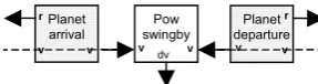
Given that the sequence of planets is defined a priori in some way, then the quantities to match are the velocity and the time.

Now, according to model 1, the final velocity in each phase is not a free variable: rather, it is an output of the model, given all the needed parameters. On the other hand, the initial velocity of each phase (both swing-by and deep space flight) is in input of the phase, and must be specified to compute that phase, as pictured schematically in Fig. 1.6.

Fig. 1.6. Block representation, with inputs and outputs, of the deep space flight phase and the powered swing-by phase for model 1.

This avoids using this model for decoupling each phase. In fact, to compute any phase the initial velocity is required. It could be arbitrarily set, but then there is no guarantee to find any set of parameters for the preceding phase which give that final velocity. The only way to guarantee the matching with this model is to compute the phases sequentially, such that the final velocity of one phase can be used as initial velocity for the following one.

The alternative is to have a model for which deep space legs and swing-bys can be computed independently, and then matched one another, to create a feasible trajectory. The aim of model 2, in particular, is to remove the dependency, for each leg, on the initial velocity. This is achieved by using a particular model, such that the deep space flight phase only requires the initial and final times, and the parameters, while the initial and final velocities are outputs. On the other hand, initial and final velocities are inputs for the swing-by model, together with the time (Fig. 1.7).

Fig. 1.7. Block representation, with inputs and outputs, of the deep space flight phase and the powered swing-by phase for model 2.

Deep space flight leg

Powered swing-by

v2

t2

v1

t1

Parameters

v1 v2

t1 t2 = t1

Parameters

Deep space

flight leg Powered swing-by

Parameters Parameters

v2

t2

v1

t1

v1 v2

(21)

1.6.1 Deep space flight with multiple manoeuvres model

[image:21.595.90.522.210.444.2]

This phase is modelled as a sequence of Lambert arcs. The first arc starts at the departure planet, and the last arc ends at the arrival planet. Each arc is connected with the following one in a point in the deep space, where a deep space manoeuvre will occur. The number of deep space manoeuvres in the phase is one fewer than the number of arcs. To compute each Lambert arc, the position (three variables) and the time (one variable) of each DSM shall be specified as parameters of the phase.

Fig. 1.8. Model 2 requires some parameters to specify the position of each DSM in a deep space flight phase, in addition to the timing.

The position of each deep space manoeuvre is specified in polar coordinates. With reference to Fig. 1.8, the three components are as following:

• Radial distance from the Sun r_DSM;

• Angle between the position vector of the first planet r_P₁ and the projection on the plane of the first planet’s orbit r_DSM′ of the position vector of the DSM r_DSM ( in-plane angle);

• Angle between the projection on the plane of the first planet’s orbit of the position vector of the DSM r_DSM′ and the position vector of the DSM itself r_DSM ( out-of-plane angle).

Rather than inputs, the initial and final velocities of the phase are the outputs of this model. The magnitude of all the deep space manoeuvres is also an output, as this is an important parameter of merit of the considered phase.

1.6.2 Powered swing-by model

P1

P2

DSM1

DSM2

1

P r

1

DSM r

2

P r

1

(22)

21

phase, and initial velocity of the following one. The idea, then, is to match the two velocity vectors with an hyperbola around the planet A minimum radius shall be given, since there is a limit on the altitude of the spacecraft on the planet (due to the surface of the planet or its atmosphere). The model tries to find a hyperbola, varying the radius of pericentre, such that the velocities at infinity are consistent with the inputs. If the hyperbola is not found, then the solution requires a manoeuvre at the pericentre (thus the name of powered swing-by). The resulting swing-by, in this case, is made by two legs of hyperbolae, connected at the pericentre through a change in velocity (Fig. 1.9).

Fig. 1.9. Schematic representation of the powered swing-by. The propelled, instantaneous manoeuvre is preformed at the pericentre of the two hyperbolas.

1.6.3 Discussion

Suppose that the problem involves the departure from planet 1, and then, with the help of the swing-by of planet 2, the spacecraft reaches planet 3. In this trajectory there are two deep space flight phases and one swing-by phase.

Given the starting time and ending time for the first deep space flight phase (between planet 1 and 2), and its parameters, the initial and final velocities of the phase can be obtained.

The second deep space flight phase (between planet 2 and 3) can be computed in the same way. Now, if the departure time is chosen to be the same as the arrival time of the preceding phase, then the two phases can be joined with a powered swing-by. This is done easily, since the incoming and outgoing velocity vectors are known: they are the final velocity for the first deep space flight phase and the initial velocity for the second deep space flight phase, respectively.

(23)

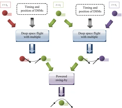
Deep space flight with multiple

0

t t= t t= ₁ t t= 2

Timing and

position of DSMs _{position of DSMs}Timing and

Deep space flight with multiple

[image:23.595.92.508.100.470.2]

Powered swing-by

Fig. 1.10. This schema represents the procedure to build a trajectory using model 2. After having fixed the times at the planets, it is possible to compute the deep space flight phases, given the parameters. Then two

consecutive deep space flight phases can be joined together through the swing-by.

1.7 Block model

In this section, a different model is proposed. Since it allows to decompose a trajectory using basic building blocks, it is a very generic model. Both model 1 and model 2 can be reproduced, together as a combination of them or other different models.

An interplanetary, multiple swing-by, multiple deep space manoeuvre trajectory can be decomposed into phases. In general, these are of 2 kinds:

• Deep space flight; • Swing-by.

(24)

23

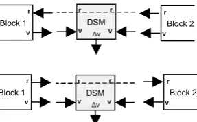
different blocks model different parts of the trajectory, or the same part, but using different models. Each block is linked with the following and the preceding one through the spacecraft state (i.e. time, position and velocity).

Let us split the trajectory as a sequence of blocks. Each block models, in a certain way, a part of the trajectory. An ordered sequence of blocks defines a complete trajectory, by modelling each part of it in a temporal sequence. All the blocks have duration (they can have zero duration, i.e. be instantaneous): in particular, a characteristic of a block is whether its duration is fixed, or it is a free parameter of the trajectory. Blocks in the sequence cannot be overlapped in time.

Each block has 2 interfaces, to join the following block and the previous block (in the temporal sequence). The interface is intended to match the state of the spacecraft between 2 continuous blocks. An interface is characterised by its type: only blocks with the same type of interface can be continuous in the sequence. This means that the interface type is a constraint for matching the blocks in the sequence.

An example of interface for a block which is modelling a deep space flight leg, is composed by position and velocity vectors of the spacecraft. For example, a propagation block with its interfaces is shown in Fig. 1.11.

Fig. 1.11. The Propagation block, given an initial position and velocity, propagates forward in time.

An interface type has a set of variables, which must be the same on all the interfaces of that type. Depending on the block, each variable on the interface can be an input or an output for that block. For the propagation block shown in Fig. 1.11, both position and velocity are inputs on the left hand side interface, while they are output on the right hand side one. This makes sense, as to propagate the trajectory, the initial position and velocity are requested (i.e., before the block), while the result of the propagation is the final position and velocity (i.e. after the block). In this document, an input is shown with an arrow going into the block, while for the output the arrow is pointing outwards. Two blocks can be consecutive in a sequence if they have the same interface type and all the inputs on the interface of one block are outputs on the interface of the other block, and vice versa. When these conditions are satisfied for all the couples of continuous blocks, then the sequence is feasible. In the representation of the blocks in the figures of this document, the sequence is feasible if the arrows, representing inputs and outputs for each block, have the same direction on the 2 consecutive interfaces of adjacent blocks, as pictured in Fig. 1.12.

The inputs on both the interfaces must be known to evaluate a block.

Fig. 1.12. An example of a feasible sequence of blocks with different types of interfaces.

Block 2

Block 1 Block 3

Propa-gation r

v v

(25)

Additionally, a block may have a set of parameters, which are also needed to evaluate the block, but they do not belong to any of the interfaces. When a block is evaluated, the outputs are then available on the interfaces. Additionally, a parameter of merit can be available as an additional output for the block.

A set of states for the spacecraft is defined between each couple of consecutive blocks in the sequence. Differently from the inputs and the outputs, the states shall be known before the evaluation of any block, for all the sequence. A particular state is the time. A block, when evaluated, can read the states at both its interfaces. If the duration of the block is not fixed, then its duration is given by the difference of the state time at its interfaces.

For example, let us consider a block which is computing a Lambert arc (Fig. 1.13). This block is a way of modelling a (part of) a deep space flight phase. Its duration is not fixed, and its interfaces may be defined with 2 quantities: the position of the spacecraft and its velocity. Since to compute a Lambert arc, the initial and final position shall be given, then we can consider that the position on both the interfaces is an input of the block. In the same way, the result of computing the Lambert arc is the velocity vector at its extrema: so, the velocities are outputs of the block. For computing a single revolution, direct Lambert arc, no parameters are needed, other than the initial and final position, and the duration. Thus, this block will not have any additional parameter.

Fig. 1.13. The Lambert block, modelling a Lambert arc. Given the initial and final position (and the time of flight, not included in the interface), computes the initial and final velocity.

For some blocks, some variables on the interface may not be relevant for evaluating the block, and the action of the block has no effect on that variable, i.e. the value of that variable is the same before and after the block. In other words, these quantities are neither input nor output for the block, but they are on the interface. In this case, we say that the block is transparent for that variable.

Let us consider for example a block which is modelling an (instantaneous) deep space manoeuvre. The aim of the block is to compute the magnitude of the DSM once the velocity before and after the deep space manoeuvre are known. This means that the velocity is an input on both the interfaces of the block. On the other hand, the block does not explicitly need the spacecraft position, and the position does not change before or after the block. This means that the block is transparent for the position, which is neither input nor output on the interfaces. The variable is represented in the figures as a dashed line connecting the two interfaces (Fig. 1.14).

Fig. 1.14. The DSM block, computing a deep space manoeuvre. The block is transparent to variable r.

When a block is transparent with respect to a variable, for example r in the case of block DSM represented in Fig. 1.14, then this variable can be either input or output on one interface of the block, but must be the opposite on the other interface, in order to

DSM r

v v

r

Δv

Lambert r

v v

(26)

25

Fig. 1.15. Two possible feasible sequences of blocks.

1.7.1 Application to the trajectory

In order to model the entire trajectory using blocks, a set of blocks shall be created, together with their interfaces. The interfaces shall be consistent one another with their inputs and outputs, and allow to reproduce a trajectory.

1.7.1.1 Interfaces

[image:26.595.228.372.99.188.2]

Three types of interface are used: they are represented in Fig. 1.16.

Fig. 1.16. The types of interfaces used to model a trajectory.

Interface 0 has no variables, and it is used on a block which is a terminator of the trajectory or a starter for the trajectory.

Interface 1 is used in the deep space flight, as in this phase the state of the spacecraft is considered to be fully characterised by its position and velocity vectors.

Interface 2 is used when the spacecraft position is supposed to be the same as a planet position. This is the case of a swing-by, for example. Since the planet and the time are states, and thus known a priori, before evaluating any block, the position of the spacecraft can be computed through the ephemerides of that planet at that time. Thus there is no need to include the position vector in the interface.

1.7.1.2 States

The states, defined between each consecutive block in the temporal sequence, are different than the inputs and outputs, as all the states can be computed before evaluating any block.

Table 1.1. States used to define a trajectory.

State Description

Time Epoch of the interface

Previous planet Planet id of the last encountered planet

Following planet Planet id of the next planet to be encountered

Current planet Planet id, if the spacecraft is considered to be at a planet; _{0, if the spacecraft is in deep space flight.}

Block 1 v r Block 1 v r Block 2 v r Block 2 v r DSM r v v r Δv DSM r v v r Δv v r v

(27)

1.7.1.3 Blocks

Fig. 1.17 shows the basic blocks composing a trajectory.

Fig. 1.17. Main blocks for modelling a trajectory.

In principle, these blocks are enough for modelling all the phases and legs of the trajectory, according to both model 1 and 2. Even though, this approach highlights that some blocks cannot be consecutive in the trajectory: for example, two Lambert arcs cannot be put next to each other because, even if they have the same type of interface, they both have positions as an input and velocities as an output (Fig. 1.18).

Fig. 1.18. Two Lambert arc blocks cannot match because of the inputs/outputs on their interface.

To avoid this problem, some other blocks were introduced. Lambert r v v r Lambert r v v r Lambert r v v r Propa-gation r v v r Launch v r dv Brake dv r v Pow swingby

dv v

v

Launch. Fixes position and velocity after the block. It requires the launch dv as an additional parameter.

Propagation. Given both position and velocity before the block, it propagates the trajectory for a certain time to obtain position and velocity after the block after the block. It requires the

Lambert Arc. It requires the positions before and after the block, and computes the velocities.

Brake. Fixes position (given by the planet ephemeris) before the block, and uses the velocity before to compute the brake manoeuvre. The dv is an additional output.

Unpowered swing-by. Given the incoming velocity, it computes the outgoing velocity. It requires 2 additional parameters to determine the swing-by.

Powered swing-by. It requires both the incoming and the outgoing velocity, and it allows a dv to match the two legs.

Unpow swingby

v v

(28)

27

Fig. 1.19. Additional blocks for modelling a trajectory.

So using these blocks, it is possible to connect 2 Lambert arcs as shown in Fig. 1.20.

Fig. 1.20. Two Lambert arc blocks connected through a Fix position block and a DSM block.

The input-output configuration on the interfaces of the Lambert arc block forces to add additional blocks to match 2 Lambert arcs. Basically a block which is fixing the position of the spacecraft (Fix position) and a block which is introducing a delta-v manoeuvre (DSM). This configuration makes sense from a physical point of view. In fact, two matching Lambert arcs require the matching point to be given, and in the same point there must be a discontinuity in the velocity vector.

1.7.1.4 Feasibility, evaluability and evaluation order

An ordered sequence of blocks is feasible if the interfaces of each couple of continuous blocks are of the same type, and each input parameter on one interface is an output in the other one, and vice versa.

The feasibility of a given sequence does not guarantee that all its blocks can be evaluated. In general we can say that a feasible sequence of blocks is evaluable if it exists an order in which the blocks can be evaluated. This order will be called evaluation order, and it is often different than the temporal order of the blocks in the sequence.

The constraint which forbids to evaluate the sequence of blocks in temporal order is the fact that a block needs all the input variables on both interfaces to be known, in order for the block to be evaluated.

Let us consider as an example the interplanetary transfer modelled with the sequence of blocks in Fig. 1.21. This sequence is temporarily ordered, in the sense that the events represented by each block happen in time with the same order of the blocks in the sequence. The sequence is clearly feasible.

Lambert r v v r Fix position r v v r r Lambert r v v r DSM r v v r Δv Fix position r v v r r Planet departure v v r Planet arrival r v v

Fix position. Force the spacecraft to pass in a point by fixing the position before and after the block (as given by the external parameter). Transparent to velocity.

Deep space manoeuvre.

Planet departure. Used when leaving a planet, it works as an interface between swing-by blocks and deep space flight blocks. Transparent to velocity, fixes the position after the block.

Planet arrival. Used when arriving at planet, it works as an interface between deep space flight blocks and swing-by blocks. Transparent to velocity, fixes the position before the block.

(29)

Fig. 1.21. Sections at which the states shall be defined.

Now we can try to evaluate each block of the sequence, considering that the inputs shall be known, and the outputs will be available after the evaluation of each block. The Launch block can be evaluated first, as it has no inputs. Its evaluation makes r and v available at section 1. r and v at the same section are inputs for the Propagation block, which can in turn be computed, giving r and v at section 2. The following block, DSM, cannot be evaluated, as the input v at its right hand side (section 3) is unknown. Note that, as the DSM block is transparent with respect to r, the value of this variable is known also in section 3: it is the same as in section 2. The block Lambert cannot be evaluated either, but it is possible to evaluate Planet arrival. This completes Lambert inputs, which in turn completes DSM inputs. Following these criteria, it results that the a possible evaluation order of the sequence is:

Launch, Propagation, Planet arrival, Lambert, DSM.

The evaluation order can be represented graphically as in Fig. 1.22 considering to have an imaginary x axis of the computational time.

Fig. 1.22. Blocks for the sequence in Fig. 1.21 positioned along a horizontal axis according to their evaluation order.

1.7.2 Reproducing other models

1.7.2.1 Model 1

Model 1 can be reproduced using some of the blocks represented in Fig. 1.17 and Fig. 1.19. The temporal sequence is represented in Fig. 1.23.

Lambert r v v r Propa-gation r v v r Launch v r dv Planet arrival r v v DSM r v v r Δv Lambert r v v r Propa-gation r v v r Launch v r dv

1 2 3 4

(30)

29

Fig. 1.23. Temporal sequence of blocks reproducing a trajectory according to model 1.

The sequence is evaluable, and it is represented in evaluation order in Fig. 1.24.

Fig. 1.24. Blocks for the sequence in Fig. 1.23 positioned according to their evaluation order.

1.7.2.2 Model 2

Model 2 can also be reproduced using the block approach. In particular, the deep space flight phase is represented in Fig. 1.25. The number of Lambert arc blocks in the phase is arbitrary.

Fig. 1.25. Sequence for a deep space flight phase of model 2

The sequence, regardless the number of Lambert arc blocks, can be evaluated in the order represented in Fig. 1.26.

Planet departure v v r Lambert r v v r Fix position r v v r r Lambert r v v r _Planet arrival r v v DSM r v v r Δv Launch v r dv Propa-gation r v v r Planet arrival r v v Lambert r v v r Unpow swingby v v

rp gamma

Planet departure v v r Propa-gation r v v r DSM r v v r Δv Propa-gation r v v r Planet departure v v r Planet arrival r v v Lambert r v v r Propa-gation r v v r Launch v r dv Unpow swingby v v

rp gamma

(31)

[image:31.595.215.359.357.395.2]

Fig. 1.26. Blocks sorted according to the evaluation order for the deep space flight phase of model 2.

The swing-by phase of model 2 is modelled using the powered swing-by block, which is between the Planet arrival block and the Planet departure blocks (Fig. 1.27). The Powered swing-by block can be evaluated when the following and the preceding deep space phases are computed. This reflects the same approach used in model 2.

Fig. 1.27. Sequence for a the swing-by phase of model 2

1.8 References

1. M. Vasile, "A global approach to optimal space trajectory design", Advances in the Astronautical Sciences, vol. 114, n. SUPPL, p. 621-640, 2003

2. M. Vasile, P. De Pascale, "Preliminary design of multiple gravity-assist trajectories", Journal of Spacecraft and Rockets, vol. 43, n. 4, p. 794-805, 2006 3. D. Izzo, V. M. Becerra, D. R. Myatt, S. J. Nasuto, J. M. Bishop, "Search space

pruning and global optimisation of multiple gravity assist spacecraft trajectories", Journal of Global Optimization, 2006

4. A. V. Labunsky, O. V. Papkov, K. G. Sukhanov, "Multiple gravity assist interplanetary trajectories", Earth Space Institute Book Series, Gordon and Breach Science Publishers, 1998

5. R. H. Battin, "An introduction to the mathematics and methods of astrodynamics, revised edition", AIAA Education Series, AIAA, New York, 1999

6. E. W. Weisstein, "Sphere point picking", Available from: http://mathworld.wolfram.com/SpherePointPicking.html, 2002 Planet departure v v r Lambert r v v r Fix position r v v r r Lambert r v v

r _Planet arrival r v v DSM r v v r Δv Pow swingby

dv v

(32)

31

PART 2 THE INCREMENTAL

APPROACH

2.1 Introduction

This part deals with the incremental approach developed by the team at University of Glasgow. The incremental approach exploits the properties of trajectory model 1. The idea is to prune the solution space incrementally, by alternately adding a leg to the trajectory, and pruning the resulting solution space.

2.2 The Incremental algorithm

The generic Δv_i in the Eq. (1.5) can be computed once the trajectory is completed up to leg i. This means that only the part of the solution vector x concerning legs 1 to i is needed, and the value up to that point is independent of the variables associated to legs

1

i+ to N_L. This allows splitting the problem into sub-problems, or levels: level 1 is taking into account the Δv associated with the launch from the departure planet and the flight to the second planet; each of the following levels takes into account a swing-by and the subsequent leg – including a DSM – to reach the next planet. Let us call D_{L i}_, the dimensional slice of the global domain D, such that it is composed only by the variables related to level i. For the model used here, the corresponding levels, variables and domains are listed in Table 2.1. Let us also define _,

1

i

i _k L k

D =

∏

₌ D , such that the trajectory up to level i is defined on the domain D_i.

Table 2.1: Levels and related variables.

Level Variables Domain

1 t₀, θ, δ , α₁, T₁ DL,1

2 γ₁, r_p_,1, α₂, T₂ D_L_,2

… … …

i γ_i−₁, rp i, 1− , αi, Ti DL i,

Let us introduce a partial objective function, for each level, of the form:

( )

1

( )

1

( )

, , 1...

i i i i i i i i L

f y = f₋ y₋ +φ y y ∈D i= N (2.1)

(33)

( )

0 1

, 1... 1

L

i

i i k L

k

N

f v v i N

f f

=

= + Δ = −

≡

∑

y

x

(2.2)

In this particular case:

( )

1

1 1 0

1

i

i i k

k

i i i

f v v

v

φ

− − −

=

= + Δ

= Δ

∑

y

but in the remainder of this part of the report it will be shown that the definition of a proper function φ_i

( )

y_i plays a very important role in the correct pruning of the solution space.

It is important to stress that the function f_i associated with level i depends only on the part of the solution vector related to the legs from 1 to i. Moreover, according to Bellman’s principle of optimality, if all the trajectory legs from 1 to i are optimal, f_i is a lower bound for f_j, when j i> , and for the whole objective function f .

Furthermore we can say that, if *

i

f is the optimal solution of a partial objective function

( )

i i

f y , and we define a threshold value f_i > f_i* and a feasible set D_i such that:

( )

{

:

}

i i i i i i

D = y ∈D f y < f (2.3)

then we can prune out the portion of the solution space that do not belong to D_i and consider for level i+1 the new solution space:

, 1

i L i

D D× ₊ (2.4)

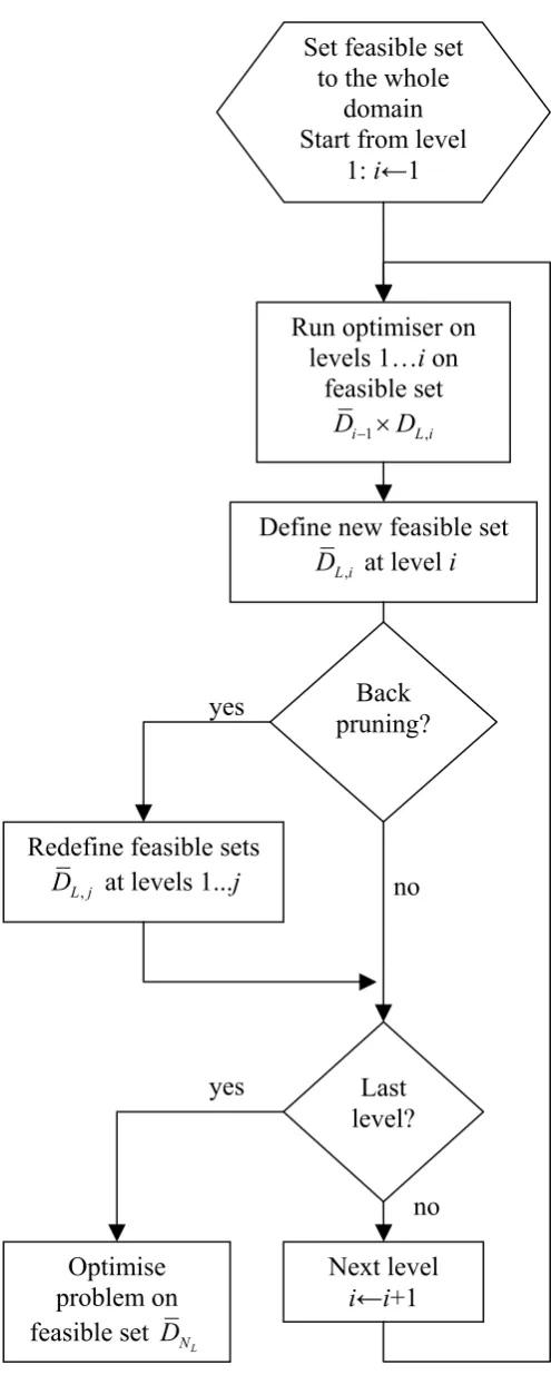
This process is called incremental pruning and f_i is called pruning threshold for level i. What makes this approach interesting is that the evaluation of a partial objective function can be remarkably less expensive than the evaluation of the function f, and the associated search space is easier to explore. Thus it is possible to analyse level 1, using

1

f on D₁ ≡D_L_,1, and ideally remove (or prune) from the search space all the sets of values for which the partial objective function is above the threshold. The result is a pruned partial domain D₁⊆D₁. Then the process continues with level 2, considering

2

f , on D D₁× _L_,2. Note that this partial domain has a smaller volume than D D₁× _L_,2, as there are sets of points in D₁ which have already been discarded during the pruning of level 1. The reduction in the search space at level i makes the search at level i+1 more efficient. At the last level, the complete objective function f is then minimised, on the remaining part of the search domain which was not pruned at previous levels, which is

L N

D .

(34)

33

(35)

Run optimiser on levels 1…i on

feasible set

1 ,

i L i

D₋ ×D

Define new feasible set

,

L i

D at level i

Next level i←i+1 Set feasible set

to the whole domain Start from level

1: i←1

Last level?

Optimise problem on feasible set

L N

D

Back pruning?

Redefine feasible sets

,

L j

D at levels 1...j

yes

[image:35.595.164.412.93.712.2]

Global trajectory optimisation: can we prune the solution space when considering deep space manoeuvres?

Global Trajectory Optimisation:

Can we Prune the Solution Space

when Considering Deep Space

Manoeuvres?

Final Report

TABLE OF CONTENTS

PREFACE

General introduction

Study objectives

Document structure

References

PART 1

MODELLING

1.1

Introduction

1.2

Modelling alternatives

1.3

Velocity formulations vs. position formulations

1.4

Common assumptions

1.5

Trajectory model 1

[ ]

(

)

[ ]

(

)

( )

∑

1.6

Trajectory model 2

1.7

Block model

1.8

References

PART 2

THE INCREMENTAL

APPROACH

2.1

Introduction

2.2

The Incremental algorithm

∏

( )

( )

( )

( )

( )

∑

( )

( )

∑

( )

( )

( )

{

}