Exact computation of one-loop correction to the energy of folded spinning string in AdS(5) x S-5

City, University of London Institutional Repository

Citation

:

10.1088/1751-8113/43/16/165402

This is the accepted version of the paper.

This version of the publication may differ from the final published

version.

Permanent repository link:

Link to published version

:

Copyright and reuse:

City Research Online aims to make research

outputs of City, University of London available to a wider audience.

Copyright and Moral Rights remain with the author(s) and/or copyright

holders. URLs from City Research Online may be freely distributed and

linked to.

City Research Online: http://openaccess.city.ac.uk/ [email protected]

arXiv:1001.4018v3 [hep-th] 2 Nov 2012

AEI-2009-127 Imperial-TP-AT-2010-01

Exact computation of one-loop correction to energy

of spinning folded string in

AdS

_×

S

M. Beccariaa,1_{, G. V. Dunne}b,2_{, V. Forini}c,3 _{, M. Pawellek}d,4 _{and A. A. Tseytlin}e,5

a

Physics Department, Salento University and INFN, 73100 Lecce, Italy

b

Department of Physics, University of Connecticut, Storrs CT 06269-3046, USA

c

Max-Planck-Institut f¨ur Gravitationsphysik, Albert-Einstein-Institut Am M¨uhlenberg 1, D-14476 Potsdam, Germany

d

Institut f¨ur Theoretische Physik III, Universit¨at Erlangen-N¨urnberg, Staudtstr.7, D-91058 Erlangen, Germany

e

The Blackett Laboratory, Imperial College, London SW7 2AZ, U.K.

Abstract

We consider the 1-loop correction to the energy of folded spinning string solution in the

AdS3part ofAdS5×S5. The classical string solution is expressed in terms of elliptic functions so an explicit computation of the corresponding fluctuation determinants for generic values of the spin appears to be a non-trivial problem. We show how it can be solved exactly by using the static gauge expression for the string partition function (which we demonstrate to be equivalent to the conformal gauge one) and observing that all the corresponding second order fluctuation operators can be put into the standard (single-gap) Lam´e form. We systematically derive the small spin and large spin expansions of the resulting expression for the string energy and comment on some of their applications.

1_{[email protected]} 2_{[email protected]} 3_{[email protected]} 4

[email protected]

5

1

Introduction

Classical string solutions in AdS5 ×S5, or non-topological solitons of the string sigma model,

play an important guiding role in the study of gauge-string duality. One of the basic examples is the folded spinning string in AdS [1, 2]. The classical string energy is a non-trivial function

of the spin, interpolating between the flat-space regime, E ∼√S+..., for small spin and the scaling AdS regime,E =S+alnS+..., for large spin. The dual gauge-theory interpretation of the latter was suggested in [1] and since then was used and verified in many papers.

The form of this spinning string solution is determined by an elliptic sn function (a solution of

the sinh-Gordon equation). Computing the quantum correction to its energy inAdS5×S5string

theory is thus a non-trivial problem, first addressed in [3]. In [3] the 1-loop correction to the energy E1(S) was expressed in terms of determinants of the bosonic and fermionic fluctuation

operators with elliptic-function potentials. It was explicitly computed only in the large-spin limit when the solution simplifies drastically (elliptic function potentials become constant). Recently,

attempts were made to compute the first few leading terms in E1(S) in the small S [9] and the

large S [10] expansions.

The aim of the present paper is to solve the problem addressed in [3], i.e. to present the

general analytic expression for the 1-loop correction E1(S) for an arbitrary value of the spin.

This would enable us to systematically expandE1 in the small S or large S limits.

The study of the largeSexpansion of string energy is important for several reasons, e.g., (i) for comparison with the Bethe ansatz predictions (see, e.g., [4, 5, 6, 7]); (ii) for further verification of the reciprocity property at strong coupling [8, 10]; (iii) for understanding the on-set of finite size

(exponential or “wrapping”) corrections in the anomalous dimension of the corresponding twist 2 gauge theory operator (cf. [11, 12, 13]) and the problem of orders of large-spin/large-coupling

limits. The study of the small S expansion may shed light on quantum corrections to quantum string states or “short” operators [9, 14].

It is also interesting to compare the explicit form of the 1-loop string correction derived directly from the string theory action with the expression coming out of the approach based on classical integrability of the string sigma model [15, 16]. The two should match in general

(see [17] and refs. there) but detailed comparison may teach us important lessons about the workings of the integrability in the case of cylindrical world-sheet topology.

We shall start in section 2 with a summary of the basic relations for the classical spinning

in the quadratic fluctuation operators, a complication of the conformal gauge expression for the 1-loop partition function of the string sigma model expanded near this solution is a mixing

of the three AdS3 modes. This mixing is absent in the static gauge [3], and we go beyond the

discussion in [3] by arguing that the conformal-gauge and the static-gauge expressions are indeed

equivalent (in particular, the string correction in the static gauge is also UV finite). This allows us to use the static gauge expression for E1 in which all 8+8 bosonic and fermionic fluctuation

modes are decoupled as a starting point of our investigation.

A further crucial observation made in section 3.3 is that all second-order fluctuation opera-tors in this stationary soliton problem can be put into the standard single-gap Lam´e ordinary

differential operator form on a circle. As discussed in section 4, this allows us to compute their determinants in an explicit way. In section 4.1 we review several equivalent forms of the general expression for the determinant of the second-order ordinary differential operator_O=₋∂2

x+V(x) on a circle: in terms of the discriminant, in terms of the quasi-momentum, in terms of the ζ -function or resolvent. In section 4.2 we specify these relations to the case of the Lam´e potential

V = 2k2sn2(x|k2). Then in section 4.3 we apply this formalism to the case of the fluctuation operators whose determinants appear in the string 1-loop correctionE1.

In section 5 we first demonstrate that the resulting expression forE1 is UV finite as expected.

We then check the equivalence between the conformal gauge and the static gauge expressions for

E1 by numerically evaluating the “mixed” conformal gauge determinant and comparing it with

its static gauge counterpart that we found analytically. We also plot E1 and compare it with

its large spin and small spin asymptotics derived analytically in sections 6 and 7. In section 6

we also check the reciprocity constraints on the few leading terms in the large spin expansion of the energy.

Some concluding remarks are made in section 8. One natural extension that we plan to address in the future [18] is to repeat the analysis of the present paper in the case of the (S, J) folded string solution with an extra orbital momentum in S5 _{[3] . This problem is more complicated}

in that even the static gauge expression for the fluctuation Lagrangian has now two mixed fluctuations and thus the standard expressions for the Lam´e operator determinant cannot be

directly applied.

There are several Appendices containing notation and technical details. In Appendix A we summarise the basic definitions for the elliptic functions, and describe the Landen

transforma-tion used to convert certain fluctuatransforma-tion operators to the Lam´e form. Appendix B describes the Gel’fand-Yaglom numerical method for computing determinants of second-order differential

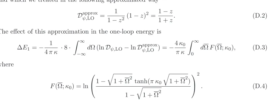
while in Appendix D we evaluate the leading correction due to the (exponentially suppressed) contributions that we neglect in the main calculation. In Appendix E we consider an alternative

approach to the expansion of the one-loop energy in the large spin limit. Appendix F relates our exact results to the perturbative expansion of the associated determinants.

2

Review of folded spinning string solution in

AdS

The folded spinning string inAdS3 space

ds2=−cosh2ρ dt2+dρ2+ sinh2ρ dφ2 (2.1)

is a classical closed string solution given by [1]

t=κ τ, φ=ω τ, ρ=ρ(σ) =ρ(σ+ 2π), (2.2)

whereκ, ωare constant parameters. The equation of motion in conformal gauge6and its solution with initial conditionρ(0) = 0 are 7

ρ′2 = κ2cosh2ρ−w2sinh2ρ, (2.3)

sinhρ(σ) = √ k

1−k2cn(ω σ+K |k

2_{) , ρ}′_{(σ) =κsn(ω σ+K|k}2_{), (2.4)}

where K ≡ K(k2_{) is the complete elliptic integral of the first kind [33], with elliptic modulus}

given by k ≡ κ

ω.8 Here ρ varies from 0 to its maximal value ρ0, which is related to the useful parameterη ork by

coth2ρ0 =

ω2

κ2 ≡1 +η≡

1

k2 . (2.5)

The periodicity implies an extra condition for the parameters

2π =

Z 2π

0

dσ= 4

Z ρ0

0

dρ

p

κ2 _cosh2_ρ−ω2 _sinh2_ρ (2.6)

integrating which one finds (see 2.5)

κ= 2k

π K, ω=

2

π K. (2.7)

6

We use Minkowski signature in both target space and world sheet, so that in conformal gauge √₋g gab =

ηab= diag(₋1,1).

7_{To construct the full (2}

πperiodic) folded closed string solution one should glue together four such functions

ρ(σ) on π

2 intervals and cover the full 0≤σ≤2πinterval. 8

The corresponding induced 2-d metric on the (τ, σ) cylinder and its curvature are

gab =ρ′2(σ)ηab , R(2) =−

∂_σ2lnρ′2

ρ′2 =−2 +

2κ2ω2

ρ′4 (2.8)

The two conserved momenta conjugate to tand φare the classical energy and the spin

E0 =

√

λ κ

Z 2π

0

dσ

2πcosh

2_ρ≡√_{λE, S=}√_{λ ω}Z 2π 0

dσ

2π sinh

2_ρ≡√_{λS (2.9)}

Using (2.3) and (2.6) we get the following explicit expressions in terms of the complete elliptic

integrals K=K(k2) andE=E(k2) (see Appendix A)

E0 =

2

π k

1−k2E, (2.10)

S = 2

π

₁

1−k2 E−K

. (2.11)

To find the energy in terms of the spin one is to solve for k (or η) in terms of S and then substitute it into the expression for the energy _E. This can be easily done in the two limiting cases:

(i) large spin or long string limit: ρ0 → ∞, i.e. η→ 0 ork→1

(ii) small spin or short string limit: ρ0 →0, i.e. η→ ∞ or k→0

In the “long string” limit when the string’s ends are close to the boundary ofAdS5, the spin

is automatically large and the parameter η is expanded around zero as

η= 2 S −

ln(8π_S)₋3

π2_S2 +... , η≪1 (2.12)

Substituting this in (2.10) one obtains for the energy the well known logarithmic behavior [1, 3,

10]

E0=S+

ln(8π_S)₋1

π +

ln(8π_S)₋1

2π2_S +... , S ≫1 , (2.13)

where the leading ln_S term is governed by the so-called “scaling function” (cusp anomaly) and

the subleading ones can be shown to obey non-trivial reciprocity relations [8, 10].

In the “short string” limit, when the string is rotating in the small central (ρ = 0) region of

AdS3, the spin is small and the parameterη is large

1

η = 2S −

1 2S

2₊7

8S

3₋117

64 S

4_{+... , η ≫1 (2.14)}

This results in the usual flat-space Regge relation [1, 3, 9]

E0 =

√

2S1 + 3 8S+...

, S ≪1. (2.15)

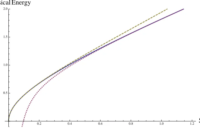
These small and large spin expansions of the classical energy_E0 are shown in Figure 1, compared

0.2 0.4 0.6 0.8 1.0 1.2 Spin 0.5

1.0 1.5 2.0

Classical Energy

Figure 1: Plot (blue, solid curve) of the classical energy_E0 as a function of the spinS, compared

with the large spin expansion (red, dotted curve) in (2.13), and the small spin expansion (gold,

dashed curve) in (2.15).

3

One-loop correction to the spinning string energy

As discussed in [3], one can compute the leading quantum correction to the energy of this solution by expanding the action to quadratic order in fluctuations near the classical solution

e

I =− √

λ

4π

Z

dτ

Z 2π

0

dσ(LBe +LFe ) (3.1)

and computing the corresponding partition function expressed in terms of determinants of the

quadratic fluctuation operators. Then (switching to the euclidean time τ _→ i τ) the 1-loop correction to the energy can be found from the 2d effective action Γ by dividing over the time

interval (t=κ τ)

E1=

Γ

κT , T ≡

Z

dτ → ∞, Γ =−lnZ (3.2)

whereZ is given by the ratio of the fermionic and bosonic determinants.

Since the above rigid spinning string solution is stationary, the coefficients in the fluctuation Lagrangian do not depend onτ. Then the relevant 2-d functional determinants may be reduced to 1-d determinants as in

ln det[−∂_σ2−∂_τ2+M2(σ)] =T

Z +∞

−∞

dΩ

2π ln det[−∂

2

i.e. we may introduce ˜Γ defined by

Γ =T

Z +∞

−∞

dΩ

2π Γ˜ . (3.4)

3.1 Conformal gauge

Following [3] one may use either the conformal gauge or the static gauge to compute the fluctu-ation Lagrangian and thus the corresponding 1-loop partition function. The bosonic fluctufluctu-ation Lagrangian reads

˜

L(conf)B =−∂a˜t∂a˜t−µt2˜t2+∂aφ∂˜ aφ˜+µ2φφ˜2+∂aρ∂˜ aρ˜+µ2ρρ˜2+

+ 4 ˜ρ(κsinhρ ∂0˜t−ω coshρ ∂0φ˜) + ∂aβu∂aβu+µ2ββu2+∂aζs∂aζs , (3.5)

µ2_t = 2ρ′2₋κ2, µ2_φ= 2ρ′2₋ω2, µ2_ρ= 2ρ′2₋ω2₋κ2, µ2_β = 2ρ′2. (3.6)

Here βu (u= 1,2) are the two AdS5 fluctuations transverse to theAdS3 subspace in which the

string is moving, while ζs (s= 1, ...,5) are fluctuations in S5. The three AdS3 fields (˜t, ρ,˜ φ˜)

are coupled so that the corresponding 1-d determinant in (3.3) will involve the following 3_×3 matrix differential operator acting on the 3 fields X= (˜t, ρ,˜ φ˜) (after τ _→iτ, ∂τ →iΩ)

Otρφ=

   

∂_σ2−Ω2−2ρ′2+κ2 2Ωκ sinhρ 0 −2Ωκsinhρ ₋∂2

σ+ Ω2+ 2ρ′2−ω2 2Ωω coshρ

0 −2Ωω coshρ −∂_σ2 + Ω2+ 2ρ′2−ω2−κ2

  

 (3.7)

In addition to the coefficients being dependent onσaccording to (2.4), this mixing makes finding the determinant of this operator a non-trivial problem. Taking into account the contribution

of the two massless conformal gauge ghosts,9 the bosonic contribution to ˜Γ = ˜ΓB+ ˜ΓF in (3.4) may be written then as

˜

Γ(conf)_B = 1 2

ln detOtρφ+ 2 ln detOβ + 3 ln detO0

, (3.8)

Oβ =−∂_σ2+ Ω2+ 2ρ′2 , O0 =−∂σ2+ Ω2 . (3.9)

The fermionic part of the quadratic fluctuation Lagrangian can be put into the form [3]

˜

LF = 2i( ¯Ψγ

a_∂aΨ−iµ

FΨ¯γ3Ψ), µF =ρ′ , (3.10)

where γa are 2-d gamma matrices (times a unit 8×8 matrix) and γ3 = diag(I,−I). It may

be interpreted as describing a system of 4+4 2-d Majorana fermions with σ-dependent masses

9

Here we are implicitly assuming that fluctuation determinants are defined with flat rather than (in general curved, forρ′

6

±ρ′. Squaring the corresponding Dirac operator, the fermionic contribution to the 2-d effective action ˜Γ in (3.4) can be written as (see also [9])

˜

ΓF =−1 2

4 ln detOψ+ + 4 ln detOψ−

, (3.11)

Oψ±≡ −∂ 2

σ+ Ω2+µ2ψ± , µ 2

ψ± =±µ

′

F +µ 2 F =±ρ

′′_+ρ′2 _{. (3.12)}

3.2 Static gauge

Another approach considered in [3] was to start with the Nambu action and use the same classical

solution but impose the static gauge on quantum fluctuations: ˜t= ˜ρ = 0. 10 In this case the remainingAdS3 mode ˜φis decoupled and is described by

˜

L(stat)φ =∂aφ∂˜ aφ˜+ ¯µ2φφ˜2 , (3.13)

¯

µ2_φ= 2ρ′2+2κ

2_ω2

ρ′2 . (3.14)

Then the static gauge analog of (3.8) takes the form (the masses of other modes are the same

as in the conformal gauge but there is no ghost determinant contribution)

˜

Γ(stat)_B = 1 2

ln detOφ+ 2 ln detOβ+ 5 ln detO0

, (3.15)

Oφ=−∂_σ2+ Ω2+ 2ρ′2+ 2κ

2_ω2

ρ′2 , (3.16)

while the fermionic contribution to 1-loop partition function is the same as in (3.12).

The advantage of the static gauge expression for the effective action is that here all fluctuation

modes are decoupled and are described by elliptic differential operators of the same type,−∂_σ2+

V(σ). On general grounds, one may expect to find the same expression for the on-shell 1-loop partition function in the two gauges.11 _{In this case one should get the following relation between}

the determinants of the conformal-gauge operator Otρφ in (3.7) and the static-gauge operator Oφ (3.16)

det_Otρφ= det_Oφ (det_O0)2 , (3.17)

where O0 is the massless operator in (3.9).12 A concern about this equality was raised in [3]

based on the fact that while the conformal gauge 1-loop partition function is UV finite [21], the

10

The classical solution of section 2 is also the solution of the Nambu action as the induced metric is conformally flat. We may define the static gauge by the condition thatτ and σ are such that tand ρ have their classical

values, i.e. do not fluctuate.

11

For example, in the case of string theory in flat target space the static-gauge Nambu and conformal-gauge Polyakov 1-loop partition functions (with nontrivial boundary conditions on a disc) are indeed the same [20].

12

static gauge one apparently contains an extra divergent term. Indeed, observing that the 1-loop logarithmic UV divergence of lnZis given by the sum of mass-squared terms and that ¯µ2

φin (3.14) may be written in terms of the curvature of the induced metric (2.8) as ¯µ2_φ = √−g(4 +R(2)), one finds that this extra divergence is proportional to Rdτ dσ √₋gR(2)_{. This is proportional}

to the Euler number of the world surface, so one may suggest [3] that it may be cancelled by the contribution of some extra “topological” factor representing the ratio of measures in the Polyakov and Nambu path integrals.

However, this extra divergence actually vanishes in the case of the cylindrical world sheet appropriate for computing the correction to the energy of a closed string state: since √₋gR(2)

is a total divergence, as long as the induced metric and thus its curvature are defined to be periodic in σ, the integral over σ should vanish.13

As we shall explicitly show in Section 5 below, the effective action in the static gauge given by the sum of (3.15) and (3.11) is indeed UV finite. Moreover, we shall also verify the relation (3.17), i.e. demonstrate the equivalence of the conformal gauge and static gauge results for the

finite 1-loop correction to folded string energy. In [3] this equivalence was seen only in the long-string (infinite-spin) limit when the solution (2.2) approaches the following asymptotic solution

[19] (ω →κ≫1)

t=κτ , φ=κτ , ρ=κσ , κ= 1

πlnS ≫1 , (3.18)

for which ρ′ _=κ=const,R(2) _{= 0 and the relation (3.17) can be easily checked.}

Proving (3.17) analytically for any κ by direct approach appears to be non-trivial. One indirect way to demonstrate (3.17) is to notice that since the corresponding quadratic fluctuation

operators appear in the linearized (near folded string solution) form of the string equations of motion in the two gauges, one may be able to relate these operators by relating the two sets of equations.

The conformal-gauge equations for small fluctuations following from (3.5)

(∂_τ2−∂_σ2) ˜t+µ2_t˜t+ 2κ sinhρ ∂τρ˜= 0 (3.19) (∂_τ2−∂_σ2) ˜ρ+µ2_ρρ˜+ 2 (κ sinhρ ∂τ˜t−ω coshρ ∂τφ˜) = 0 (3.20) (∂_τ2−∂_σ2) ˜φ+µ_φ2φ˜+ 2ω coshρ ∂τρ˜= 0 , (3.21)

13

More explicitly, here the relevant integral isR2π

0 dσ(lnρ

′ )′′

= [(lnρ′)′ ]2π

0 = [ρ

′′

ρ′]

π/2

0 + [

ρ′′

ρ′]

π π/2+ [

ρ′′

ρ′] 3/2π

π +

[ρ′′

ρ′] 2π

3/2π, whereρ ′′

= (κ2

−ω2_{) sinh}

ρcoshρ, ρ′=_±pκ2_cosh2

ρ−ω2_sinh2

should be supplemented with the conformal gauge conditions (Virasoro constraints)

−κ cosh2ρ ∂τ˜t+ (ω2−κ2) sinhρcoshρρ˜+ρ′∂σρ˜+ω sinh2ρ ∂τφ˜= 0 (3.22) −κ cosh2ρ ∂σ˜t+ω sinh2ρ ∂σφ˜+ρ′∂τρ˜= 0. (3.23)

The latter should allow one, in principle, to eliminate the two modes (say ˜t and ˜φ) in terms of the third one (˜ρ), getting an effective equation for the latter. Since theρ-background does not depend onτ and since the above equations are linear we may do this elimination at the Fourier mode level, i.e. replacing ˜t _→ eiΩτ_{¯t(σ), φ}˜ _{→ e}iΩτ_φ¯_{(σ), ρ˜ → e}iΩτ_{ρ¯(σ). Then (3.22),(3.23)} imply (changing to euclidean time notation, i.e. Ω→iΩ)

¯

t = sinhρ 2κΩ

∂_σ2−2ρ′∂σ+κ2−ω2−Ω2

¯

ρ , (3.24)

¯

φ = −coshρ 2ωΩ

∂_σ2+ 2ρ′∂σ−κ2+ω2−Ω2

¯

ρ . (3.25)

Substituting this into the equations of motion (3.19)-(3.21) we find that one of them is satisfied

automatically while the other two become equivalent to the following fourth-order differential equation for ˜ρ, i.e. _O(4)ρ¯= 0, where

O(4)≡∂_σ4+ 2(ω2+κ2−Ω2−4ρ′2)∂_σ2−8ρ′ρ′′ ∂σ +κ4+ (Ω2+ω2)2+ 2κ2(Ω2−ω2) . (3.26)

Remarkably, this operator can be factorized as a product of two second-order operators as

follows:

O(4)=_O1· O2 , O1 = (ρ′)−1 Oφ ρ′ , O2 =ρ′ O0 (ρ′)−1 , (3.27)

where Oφ and O0 are the same as the static-gauge operator in (3.16) and the massless mode

operator in (3.9), respectively. The algebraic ρ′ _{and (ρ}′₎−1 _{factors may be attributed to a}

change of normalization of the corresponding fluctuations.14 This way we see how the static gauge operator_Oφ emerges from the mixed conformal gauge fluctuation operator, i.e. provides

support for the relation (3.17).

In Section 5 below we shall verify that the effective action in the static gauge is indeed UV finite, and we demonstrate the equivalence (3.17) between the conformal gauge and the

static gauge results for the finite 1-loop correction to the folded string energy by computing the corresponding functional determinants.

14

A similar discussion could be given at the level of path integral with the conformal gauge condition accounted for by two delta-functions (as appropriate if one starts with the Nambu path integral). The step analogous to (3.24),(3.25) would then produce an extra det_O0 factor as required for balance of degrees of freedom. For

3.3 Lam´e form of the second-order fluctuation operators

To summarize, the simplest starting point for computing the 1-loop correction to the folded string energy is thus its representation in terms of the 1-loop effective action in the static gauge

given by the sum of (3.15) and (3.11), i.e. is expressed in terms of determinants of the following three types of operators defined on periodic functions f = (β, φ, ψ_±)

Of =₋∂_σ2+Vf(σ) + Ω2 , f(σ) =f(σ+ 2π) , (3.28)

where (using the form of the classical solution (2.4))

Vβ = 2ρ′2 = 2κ2sn2(¯σ|k2) , σ¯≡ω σ+K, (3.29)

Vφ= 2ρ′2+ 2κ2_ω2

ρ′2 = 2κ

2_sn2_(¯σ|k2_{) + 2ω}2_ns2_(¯σ|k2_{) , (3.30)}

Vψ± =ρ′

2_±ρ′′ _=κ2_sn2_(¯σ|k2_{)±κ ωcn(¯σ|k}2_{) dn(¯σ|k}2_{) . (3.31)}

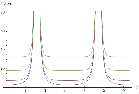
These potentials are plotted in Figures 2, 3, 4 where we have chosen four particular values of

the elliptic modulusk= κ_ω=0.5, 0.9, 0.99, 0.999.

1 2 3 4 5 6 Σ

5 10 15

VΒHΣL

Figure 2: Potential Vβ in (3.29), for k= 0.5,0.9,0.99 and 0.999, from bottom to top.

It is convenient to introduce the rescaled spatial variable (cf. (2.7))

x≡ω σ= 2K

π σ , (3.32)

and write _Oβ as (we ignore a trivial overall constant factor)

Oβ =−∂_x2+ 2k2sn2(x+K|k2) + π

2_Ω2

1 2 3 4 5 6 Σ 20

40 60 80

VΦHΣL

Figure 3: PotentialVφin (3.30), for k= 0.5,0.9,0.99 and 0.999, from bottom to top. Note that singularities appear at the turning points whereσ = n+1₂π.

1 2 3 4 5 6 Σ

-5 5

VΨHΣL

Figure 4: Potentials Vψ+ (red) andVψ− (blue) in (3.31) , for k = 0.5,0.9,0.99 and 0.999, from

which is now defined on the periodic functions β(x) = β(x+ 4K). The expression in (3.33) is recognized as being a Lam´e differential operator in thesingle-gap form (which will be reviewed in the next section).

Remarkably, all other fluctuation operators entering the effective action, i.e. _Oφ and _Oψ±,

whose structure is apparently much more involved, can also be cast into the single-gap Lam´e form. Their transformation has several steps involving rescaling the coordinate and the elliptic

modulus a special way, see (A.18)-(A.21) forOφ, and (A.22)-(A.31) forOψ±.

We can summarize the results as follows: each (static gauge) fluctuation operator is a

single-gap Lam´e operator with the following periodic eigenvalue problem

h

−∂_x2+ 2 ¯k2sn2(x|¯k2) + ¯Ω2ifΛ(x) = ΛfΛ(x) , fΛ(x) =fΛ(x+L), (3.34)

wherex is a rescaledσ variable with periodLand ¯kand ¯Ω are rescaled modulus and euclidean frequency in (3.29)-(3.31), namely,

(a) for the bosonic operator Oβ:

x= 2K

π σ+K, k¯=k , Ω¯

2 ₌πΩ

2K

2

, L= 4K (3.35)

(b) for the bosonic operator_Oφ: the elliptic modulus is ˜k2= ₍₁₊4k_k)2 and

x= 2Ke

π σ+iK˜

′_, ¯_{k= ˜k≡} 2 √

k

1 +k , Ω¯

2₌πΩ

2Ke

2

+ ˜k2, L= 4Ke (3.36)

(c) for the fermionic operators _Oψ±:

x=

  

e

K

π σ+ e

K

2, forψ+

e

K

π σ+3 e

K

2 , forψ−

, ¯k= ˜k_≡ 2

√

k

1 +k , Ω¯

2₌πΩ

e

K

2

+ ˜k2, L= 2Ke (3.37)

Here Ke ≡K(˜k2), andk′_≡√1₋k2_{, see Appendix A for notation and details.}

As we shall discuss in the next section, the remarkable feature of this Lam´e spectral problem

(3.34) is that it can be solvedexactly, and hence the corresponding determinant can be computed

analytically (with a result that is independent of constant shifts in the coordinates).

4

Determinants of single-gap Lam´

e operators

Below we shall first review the method that allows one to compute the determinant of a single-gap Lam´e operator without having to solve the corresponding spectral problem explicitly. We will then apply this technique to the computation of determinants of the fluctuation operators

4.1 Floquet theory of determinants of 2-nd order one-dimensional operators

Consider the following eigenvalue problem for an ordinary differential operator,O=−∂_x2+V(x), with a periodic potential

−∂_x2+V(x)f(x) = Λf(x), V(x+L) =V(x) . (4.1)

For either periodic or antiperiodic boundary conditions onf(x), we find a discrete spectrum of eigenvalues {Λn}, and the associated determinant is then formally given by DetO=Q_nΛn.

Given a general potential V(x) it is of course difficult to find the eigenvalues, and even given the eigenvalues, the infinite product must be regulated. Both difficulties can be overcome in the following way. Consider two independent solutions f1,2(x; Λ) to (4.1) satisfying the conditions

f1(0; Λ) = 1, f1′(0; Λ) = 0 ,

f2(0; Λ) = 0, f2′(0; Λ) = 1, (4.2)

wheref′ _{=∂xf. Then thediscriminant ∆(Λ) of the operator O is defined as [34]}

∆(Λ) =f1(L; Λ) +f2′(L; Λ) (4.3)

The periodic and the antiperiodic eigenvalues are given by the following (in general

transcen-dental) equations:

∆(Λ) =

  

+2 (periodic)

−2 (antiperiodic)

(4.4)

Remarkably, the determinant can be computed without knowing these eigenvalues explicitly. Indeed, the Hill determinant, i.e. the ratio of determinants with non-zero V and V = 0 has a simple expression in terms of the discriminant [34]:

det[₋∂_x2+V(x)₋Λ] det[₋∂2

x−Λ]

= ∆(Λ)−2

−4 sin2_(L√_Λ/2) (periodic) (4.5)

det[₋∂2

x+V(x)−Λ] det[−∂2

x−Λ]

= ∆(Λ) + 2

4 cos2_(L√_Λ/2) (antiperiodic) (4.6)

In what follows we shall always assume that determinants we consider are normalized to the trivial free determinant det[₋∂2

x], and thus omit the resulting Λ− and V-independent overall constant (such constants will cancel in the string partition function due to balance of the degrees of freedom). Then we may write the above relations simply as

det_P,AP[−∂_x2+V(x)−Λ] =

 



∆(Λ)−2 (periodic)

∆(Λ) + 2 (antiperiodic)

It is useful to relate this representation for the determinant to a familiar physical notion of “quasi-momentum”. By the Floquet/Bloch theory [34], the equation (4.1) has two independent

solutions of the formf_±(x) =e±i p(Λ)xχ_±(x), whereχ_±(x) are periodic, so that under translation through one period the Bloch solutionsf_±(x) change by a phase

f_±(x+L) =e±ip(Λ)L f_±(x) (4.8)

where, by definition, p(Λ) is the “quasi-momentum”. Then ∆(Λ) = 2 cos(L p(Λ)), and we can re-write (4.7) in terms of the quasi-momentum as follows [34]:

det_P,AP[₋∂_x2+V(x)₋Λ] =

  

−4 sin2 L₂ p(Λ) (periodic) +4 cos2 L

2 p(Λ)

(antiperiodic)

(4.9)

Thus, knowing the quasi-momentum p(Λ) amounts to knowing the discriminant and also the determinant.

Another interesting and useful relation is the link between the determinant and the

discrimi-nant through the contour integral representation for the spectral zeta function. For definiteness, let us consider the case of the periodic boundary conditions. Then the spectral zeta function is

ζ(s) = 1 2πi

Z

γ

dΛ Λ−s ∂

∂Λln [∆(Λ)−2] = 1 2πi

Z

γ

dΛ Λ−s R(Λ), (4.10)

where the resolvent

R(Λ) = ∆′(Λ)

∆(Λ)₋2 (4.11)

has simple poles exactly at the values of Λ corresponding to the points of the periodic spectrum.

The contour γ in (4.10) runs counter-clockwise above and below the positive real axis enclosing all poles of the resolvent. Wrapping the contour along the branch cut along the negative real line gives [25]

ζ(s) =₋sin(πs)

π

Z _∞

0

dΛ Λ−s R(₋Λ). (4.12)

According to the zeta function definition of the functional determinant

det₋∂_x2+V(x)=e−ζ′(0) (4.13)

to compute the determinant we need to know

−ζ′(0) =₋

Z _∞

0

dΛ ∂

∂Λln [∆(−Λ)−2] = ln

[∆(0)₋2]

[∆(−∞)−2] (4.14)

Here we subtracted the divergent term ln[∆(_−∞)₋2] by assuming that we again divide by a

“free” reference determinant. Then finally

detP

Shifting the potential by a constant −Λ, we reproduce the representation in (4.7).

The important feature of the above expressions is that the determinants can be calculated in

closed form without computing any of the eigenvalues. There is yet another way to compute the determinants, known as the Gel’fand-Yaglom method [30, 38], which for periodic systems

re-duces essentially to a numerical evaluation of the discriminant giving the determinants via (4.7). This method is described in Appendix B, where we also consider systems of coupled equations,

which will be important for demonstrating explicitly the equivalence of the computation in the conformal and static gauges.

It is useful to illustrate the above general relations on the simple example of constant potential

V(x) =m2, x_∈(0, L) . (4.16)

Then the two independent solutions in (4.2) are f1(x; Λ) = cosh(

√

m2_{−Λx) and f}

2(x; Λ) =

sinh(√m2_−Λx)/√_m2_{−Λ. Therefore, the discriminant (4.3) and the determinants (4.9) are}

∆(Λ) = 2 cosh(Lpm2_{−Λ), (4.17)}

det_P,AP(−∂_x2+m2−Λ) =

  

 

4 sinh2L₂ √m2_−Λ

4 cosh2L₂ √m2_−Λ

(4.18)

The quasi-momentum in (4.8) here is p(Λ) = √Λ₋m2_{, so these relations are consistent with}

(4.9). Furthermore, in this case we know the explicit eigenvalues (n∈Z):

Λn=

  

m2+ 2nπ_L 2 (periodic)

m2₊ (2n+1)π L

2

(antiperiodic)

(4.19)

Then the expressions in (4.18) also follow from the infinite product representations for the sinh

and cosh functions, combined with zeta function regularization.

4.2 Case of single-gap Lam´e potential V₍x_{) = 2}k2_sn2₍x_|k2₎

The important example which is our main interest here is provided by the single-gap Lam´e operator in (3.34), i.e.

h

−∂_x2+ 2k2sn2(x|k2)if(x) = Λf(x). (4.20)

The two independent Bloch solutions of (4.20) here are [33]

f_±(x) = H(x±α) Θ(x) e∓

whereH,Θ, Z are the Jacobi Eta, Theta and Zeta functions defined in (A.10), andα=α(Λ) is given implicitly by

sn(α_|k2) =

r

1 +k2_−Λ

k2 . (4.22)

Using the period properties of the Jacobi functions (A.12) we see that

f_±(x+ 2K) =₋f_±(x)e∓2KZ(α) _≡ f_±(x)e2iKp(α) , (4.23)

which defines the quasi-momentum as

p(Λ) =i Z(α|k2) + π

2K . (4.24)

Therefore, from (4.9) we immediately find analytic expressions for the determinants. Assuming the period is L= 2K, we find

det(_P,APL=2K)h₋∂_x2+ 2k2sn2(x_|k2)₋Λi=

  

−4 cosh2[KZ(α|k2)]

−4 sinh2[KZ(α_|k2_)] (4.25)

where the relation between Λ and α is given by (4.22). On the other hand, for the period

L= 4K, we find

det(_PL=4K)h₋∂_x2+ 2k2sn2(x_|k2)₋Λi= 4 sinh2[2KZ(α_|k2)] (4.26)

Note that this is the same as the product of the periodic and antiperiodic determinants (4.25) with the period 2K, as it should be.

The periodic potential in (4.20) has the special property that its band spectrum has only a single gap, and is known therefore as a one-gap potential, as illustrated in Fig. 5. The spectrum

has three band edges (which are also the lowest eigenvalues of the periodic spectrum of the problem on the interval 4K):

Λ1 =k2 , Λ2 = 1 , Λ3 = 1 +k2 . (4.27)

One can rewrite the relation between Λ and α in (4.22) in terms of the band edges as follows

ksn(α;k2) =

r

1

2(Λ1+ Λ2+ Λ3)−Λ. (4.28)

The resolvent is

R(Λ) = d

dΛ ln [∆(Λ)−2] =L

dp dΛ cot

L

2 p(Λ)

L=k2

L=1 L=1+k2

L=Μ

2 4 6 8 10 L

-4

-2 2 4 6 8

DHLL

Figure 5: The discriminant ∆(Λ) for the Lam´e potential V(x) = 2k2_sn2_(x|k2_{) with k= 0.9.}

The three band edges occur at the points Λ1,Λ2,Λ3 where ∆(Λ) cuts the lines ±2, while the

remainder of the periodic/antiperiodic spectrum consists of points where ∆(Λ) touches the lines ±2.

We can also expressdp/dΛ simply in terms of the band edges:

dp dΛ =i

Λ₋µ

2p(Λ1−Λ)(Λ2−Λ)(Λ3−Λ)

(4.30)

where

µ= 1 2

Λ1+ Λ2+ Λ3− hVi

, hVi ≡ 1

L

Z L

0

V(x)dx (4.31)

To see this, note that from (4.8)

dp dΛ =

dp dα

dα dΛ =i

dZ(α_|k2)

dα

dα dΛ =i

1₋k2sn2(α_|k2)₋ E(k

2₎

K(k2₎

dα dΛ

where we have used the definition (A.16) of the Zeta function. Also, from (4.28) we have

dα dΛ =

1

2k2_dn(α|k2_{) cn(α|k}2_{) sn(α|k}2₎ =

1

2p(Λ1−Λ)(Λ2−Λ)(Λ3−Λ)

.

Finally, for the potentialV(x) = 2k2_sn2_(x|k2_{) we find for L= 2K}

hVi= 1

L

Z L

0

dx2k2sn2(x|k2) = 21− E(k

2₎

K(k2₎

, (4.32)

and the same forL= 4K. Thus, taking into account (4.27), we get

µ=k2+ E(k

2₎

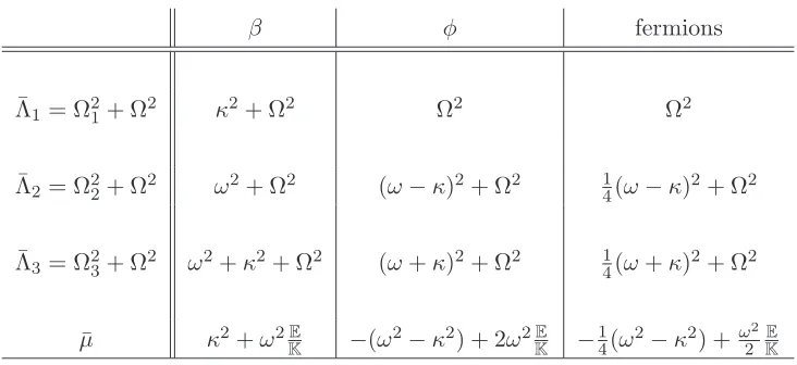
β φ fermions

¯

Λ1= Ω21+ Ω2 κ2+ Ω2 Ω2 Ω2

¯

Λ2= Ω22+ Ω2 ω2+ Ω2 (ω−κ)2+ Ω2 14(ω−κ)2+ Ω2

¯

Λ3= Ω23+ Ω2 ω2+κ2+ Ω2 (ω+κ)2+ Ω2 14(ω+κ)2+ Ω2

¯

µ κ2+ω2E

K −(ω

2_−κ2_{) + 2ω}2E K −

1

4(ω2−κ2) +ω

2

2 KE

Table 1: The lowest (analytically known) eigenvalues of the fluctuation operators

Thus we obtain a compact expression for the resolvent of the single gap Lam´e potential with

periodL in terms of the quasi-momentump(Λ) and the band edges as

R(Λ) = L 2

Λ₋µ

p

(Λ1−Λ)(Λ2−Λ)(Λ3−Λ)

cothL p(Λ) 2i

. (4.34)

4.3 Results for determinants of static-gauge fluctuation operators

Let us now apply the above results to the case of the fluctuation operators defined by (3.34)-(3.37). The results in Eqs. (4.22) and (4.25)-(4.26) are actually all that we need in order to write

downexact analytic expressions for the determinants of these operators. The analytically known

eigenvalues or band edges can be obtained from (4.27) with the appropriate shifts (Λi →Λi−Ω¯2) and rescalings, and an analogous procedure applies to the corresponding resolvents in (4.34).

The results can be summarized as follows.

(a) for the β operator, in view of (3.35), the determinant reads

detOβ(Ω) = 4 sinh22KZ(αβ|k2)

, (4.35)

sn(αβ;k2) =

q

1 +k2_{+ (}πΩ 2K)2

k . (4.36)

The band edges are obtained from (4.27) by shifting and rescaling

¯ Λi=

_2K

π

2

(Λi+ ¯Ω2)≡ Ω2i + Ω2 , Ω¯2 =

_πΩ

2K

2

(4.37)

the eigenvalues in the first column of Table 1 that can now be re-expressed in terms of the parameters of the classical solution

{Λ¯1,Λ¯2,Λ¯3} =

_2K

π

2n

k2+ ¯Ω2,1 + ¯Ω2,1 +k2+ ¯Ω2o

≡ nκ2+ Ω2, ω2+ Ω2, κ2+ω2+ Ω2o. (4.38)

(b) For the φ operator in (3.36) we have ˜k2= _(k+1)4k 2, and thus

detOφ(Ω) = 4 sinh22KeZ(αφ|˜k2)

, (4.39)

sn(αφ|˜k2) =

q

1 + (πΩ

2Ke)

2

˜

k . (4.40)

The band edges are obtained from (4.27) by shifting and rescaling

¯ Λi=

_2Ke

π

2

(Λi+ ¯Ω2)≡ Ω2i + Ω2 , Ω¯2 =

_πΩ

2Ke

2

+ ˜k2 , (4.41)

getting thus the eigenvalues in the second column of Table 1.

(c) For the ψ_± operators in (3.37) the elliptic parameter is ˜k2 = _(k+1)4k 2, and we get

det_Oψ(Ω) =₋4 cosh2eKZ(αψ|k˜2), (4.42)

sn(αψ|˜k2) =

q

1 + (π_eΩ

K ) 2

˜

k . (4.43)

Since the determinant is independent of constant shifts of coordinates like the one in (3.37)

(see, e.g., Appendix B) the expressions for the determinants ofOψ− andOψ+ are the same

and therefore we will not distinguish them in what follows. The band edges follow from

(4.27)

¯ Λi =

e_K

π

2

(Λi+ ¯Ω2)≡ Ω2i + Ω2, Ω¯2=

_πΩ

e

K

2

+ ˜k2 (4.44)

5

Exact expression for one-loop correction to string energy

As follows from the above discussion (see (3.2),(3.15),(3.11),(4.35),(4.39),(4.42)) the 1-loop

cor-rection to the energy of the folded spinning string may be written as

E1 =−

1 4πκ

Z _∞

−∞

dΩ ln det

8_Oψ

detOφ det2Oβ det5O0

where κ = 2_πkK, K = K(k2) (see (2.7)) and the determinants as functions of Ω have the following explicit expressions15

det_Oβ = 4 sinh22KZ(αβ|k2)

where sn(αβ|k2) =

q

1 +k2_{+ (}πΩ 2K)2

k (5.2)

detOφ = 4 sinh2h2KeZ(αφ|k˜2)

i

where sn(αφ|k˜2) =

q

1 + (πΩ

2Ke)

2

˜

k (5.3)

detOψ = −4 cosh2hKeZ(αψ|˜k2)

i

where sn(αψ|k˜2) =

q

1 + (π_eΩ

K ) 2

˜

k (5.4)

det_O0 = 4 sinh2[πΩ] (5.5)

The computation ofE1 is thus reduced to inverting the transcendental equations for αβ, αφ, αφ, finding the corresponding values ofZ-function (A.15). The integral is then a function of k= _ωκ and Ω.16 _{Doing the integral over Ω we then end up with a function ofkonly or the spin (2.11).}

It is straightforward to evaluate the Ω integral numerically, as discussed below.

5.1 UV finiteness

Let us first check that the resulting expression forE1 is indeed UV finite, i.e. the integral over

Ω is convergent at infinity. The large Ω behavior of the determinant factors in (5.1) can most easily be extracted from the general large Ω behavior of the associated resolvents. Changing

variable from Λ to −Ω2, we define

R(Ω)≡ −2 ΩR(−Ω2) (5.6)

Then we find from (4.34) that the general structure of the expansion is

R(Ω) =r0+

r1

Ω2 +

r2

Ω4 +O(Ω−

6_{) , Ω→ ∞ (5.7)}

r0 = 2π , r1 = 2π

¯

µ₋1

2(¯Λ1+ ¯Λ2+ ¯Λ3)

= 2π_hV_i (5.8)

Therefore, the large Ω behavior of the log determinant is

ln det_O=r0Ω−

r1

Ω +O(Ω−

3_{), Ω→ ∞ (5.9)}

15

The determinant of the massless operatorO0 is found by taking the regularized infinite product of its

eigen-valuesλn=n2+ Ω2.

16

Note that in the limit whenk= 0, i.e. potentials vanish all determinants take the same value as det_O0, i.e.

Using the corresponding values of ¯µand Li of the three non trivial fluctuation modes given in Table 1, we find [we have also used the elliptic identities (A.28)–(A.29)]:

ln det_Oβ = 2πΩ + 4ω(K−E) Ω−1+_O(Ω−3), (5.10) ln det_Oφ = 2πΩ + 8ω(K−E) Ω−1+_O(Ω−3), (5.11) ln detOψ = 2πΩ + 2ω(K−E) Ω−1+O(Ω−3) , (5.12)

ln detO0 = 2πΩ +O(Ω−3) . (5.13)

The leading (quadratically divergent) terms cancel in (5.1) due to the balance of world-sheet degrees of freedom in (5.1). The subleading (logarithmically divergent) terms also cancel in the

combination appearing in (5.1), (2×4 + 8−8×2)(K−E) Ω−1 = 0. We thus confirm that the static gauge result for the 1-loop energy is indeed UV finite, as was argued in section 3.2.

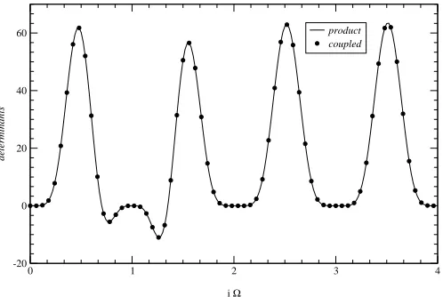
5.2 Equivalence between the static gauge and conformal gauge results

To check the equivalence between the static gauge and conformal gauge results one needs to verify the factorization relation (3.17). This can be done numerically, as follows. To evaluate

the left hand side of (3.17) we used the Gel’fand-Yaglom method (for details, see Appendix B) to compute numerically the determinant of the operator _Otρφ in (3.7) as a function of Ω for

various values of k. The right hand side of (3.17) can be computed directly using the expression for the determinant of_Oφ found above (5.11). We find perfect agreement. In Figure 6 we have

plotted the expressions on both sides of (3.17) as functions of Ω fork= √1

10. Similar agreement

is found for anyk.

5.3 General form of the 1-loop correction E₁

Going back to the complete expression for E1 in (5.1) it is useful, in order to safely expand in

one of the interesting limits analyzed below, to separate there the contributions of the massless modes of _O0 (i.e. Ω2) and the lowest eigenvalues (¯Λ1 in Table 1) ofOβ,Oφ and Oψ. Then we

get

E1 =−

1 4πκ

Z _∞

−∞

dΩ

ln (det

′_Oψ)8

det′_Oφ(det′_Oβ)2 _(det′_O

0)5

+h(Ω)

(5.14)

where

det′Oβ,φ,ψ ≡ detOβ,φ,ψ_¯ Λ1

, det′O0 ≡

detO0

Ω2 (5.15)

0 1 2 3 4 i Ω

-20 0 20 40 60

determinants

product coupled

Figure 6: Comparison between the left-hand-side and the right-hand-side of Eq.(3.17), for

k= √1

10. The circles represent the numerical Gel’fand-Yaglom result for the determinant detOtρφ

of the three coupled fluctuations in conformal gauge, while the solid line is a plot of the

corre-sponding analytic static gauge expression, given by the product of the determinant (5.3) for the massive fluctuationφand the square of the determinant (5.5) of a massless mode. To emphasize the precision of the agreement we have plotted the oscillatory form, as a function of iΩ.

Using that

Z _∞

−∞

dΩh(Ω2) =₋4π κ (5.17)

the one-loop correction to the energy (5.1) takes the form

E1 = 1−

1 4πκ

Z _∞

−∞

dΩ ln (det′Oψ)

8

det′Oφ (det′Oβ)2 _(det′_O

0)5

. (5.18)

This expression is straightforward to evaluate numerically for various values of k or the spin_S in (2.11), and thus to plotE1.

To gain more analytic control over the form ofE1as a function of spinS we may consider the

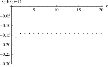
expansion of it in the large spin (“long string” ork_→1) limit or in the small spin (“short string” or k→ 0) limit. This will be done in detail in the following two sections 6 and 7 respectively. In figure 7 we presented together the results – the plots ofE1(k) found analytically in the large

spin expansion (right-most green curve) and in the small spin expansion (left-most red curve) and also the plot of the exact E1 found numerically from (5.18) (blue curve connecting the two

0.2 0.4 0.6 0.8 1.0 k

-2

-1 1

E1

Figure 7: Plots of E1 as a function of k: the blue, solid, curve is found numerically from the

exact expression (5.18) for generic values ofk; the green, dotted, curve is found from an analytic expansion in the k→1 or large spin limit, using the first two terms in (6.36); the red, dashed, curve is found from an analytic expansion in thek _→0 or small spin limit, using the first two terms in (7.7). The agreement is excellent in both extreme limits.

2 4 6 8 10 Spin

-2.0

-1.5

-1.0

-0.5

0.5 1.0

1-loop Energy

Figure 8: Plots ofE1as a function of the classical spinS. The solid, blue curve is the exact result,

6

Large spin expansion

This limit (see (2.12)) is defined as k→1 or, equivalently, η→0 in (2.5).

6.1 Leading order

In this subsection we will compute the leading term in k_→1 expansion ofE1 in (5.1) and also

comment on first exponential subleading terms.

At the leading order the classical solution is approximated by

ρ′_≈κ0 , ρ′′ ≈0 , ω ≈κ≈κ0 , κ0=

1

π ln

16

η → ∞. (6.1)

If we use these limiting expressions directly in the fluctuation operators then we conclude that their potential terms become constant

Oβ,0=−∂σ2+ 2κ20+ Ω2 , Oφ,0 =−∂σ2+ 4κ20+ Ω2 , Oψ±,0 =−∂ 2

σ+κ20+ Ω2 (6.2)

and thus we find from (5.1) [3]

E₁(0) = 1 2κ0

∞ X

n=−∞ hq

n2_{+ 4κ}2 0+ 2

q

n2_{+ 2κ}2 0+ 5

√

n2₋₈q_n2_+κ2 0

i

(6.3)

where we performed the integration over Ω before commuting the determinants defined on a unit circle. Using the Euler-MacLaurin formula to transform the sum into an integral one finds

E₁(0)= 1

κ0

h

−3κ2₀ ln 2 ₋ 5

12+O(e−

2πκ0₎i_{, κ}

0 → ∞, (6.4)

where the leading term is the result of [3] and the subleading term appeared in [22].

Let us now see what we get if we start instead with the exact expressions for the determinants (5.2)-(5.4). Using the expressions collected in Appendix C (see (C.8)-(C.10)), we get at the

leading order

2K(k2)Z(αβ|k2) ≈ π κ0x with x=

s

2 + Ω

2

κ2 0

, (6.5)

2K(˜k2)Z(αφ|k˜2) ≈ π κ0y with y=

s

4 +Ω2

κ2₀ , (6.6)

K(˜k2)Z(αψ|k˜2) ≈ π κ0z with z=

s

1 + Ω

2

κ2₀ , (6.7)

which would give, once substituted into (5.2)-(5.4), the following expressions for the determinants

det_Oβ(Ω2) _≈ 4 sinh2[π κ0x] (6.8)

det_Oφ(Ω2) _≈ 4 sinh2[π κ0y] (6.9)

Integrating logarithms of (6.8)-(6.10) over Ω one gets the result that may be represented also as

E1 ≈E˜1(0) =

1 2κ0

∞ X

n=−∞ hq

n2_{+ 4κ}2 0+ 2

q

n2_{+ 2κ}2 0+ 5

√

n2₋₈q_(n+1

2)2+κ20

i

. (6.11)

Here the shiftn_→n+1₂ in the fermionic contribution is due to the cosh2 instead of sinh2 form of the determinant (6.10).17 _{While this shift does not affect the result for the two leading terms}

in (6.4), it formally changes the form of the subleading corrections (which should not, however, be trusted in the approximation used to arrive at (6.11)).

Indeed, there is of course no contradiction as the approximation used to derive (6.4) was supposed to be valid only for the leading term in largeκ0 expansion, i.e. the expressions for the

subleading terms should not be trusted a priori. Still, let us briefly comment on the exponential

corrections to the first two leading terms in (6.4) comparing what follows from (6.3) to what follows from (6.11). As was found in [29] usingζ-function regularization of the sums in (6.3)

E₁(0)=−3κ0ln 2−

5 12κ0 −

1 π ∞ X n=1 1 n h

K1(4πnκ0) +

√ 2K1(2

√

2πnκ0)−4K1(2πnκ0)

i

, (6.12)

whereK1 is the Bessel function of the second type

Z _∞

m

dxpx2_−m2_e−2πkx₌ m

2πkK1(2πkm). (6.13)

The K1 terms represent the exponential corrections since

K1(y)→

r

π

2ye−

y _{1 +O(y}−1_{), y→ ∞. (6.14)}

Repeating the same computation in the case of (6.11) one finds that

˜

E₁(0) =E₁(0)+ 4

π

∞ X

n=1

[(₋1)n₋1]K1(2πnκ0). (6.15)

6.2 Beyond the leading order

To find subleading corrections in large κ let us add and subtract the leading order contribution (6.4) from the expression (5.1):

E1 =

1

κ[−3κ

2 0 ln 2−

5

12 +O(η

2_{)] +E}(sub)

1 , κ0 → ∞ (6.16)

E₁(sub) = − κ0 4πκ

Z _∞

−∞

d ¯Ω ln D

8 ψ D2 βDφ . (6.17) 17

This shift may be formally interpreted by saying that fermions have antiperiodic boundary conditions, so that ln det(₋∂2

σ+ Ω2+κ20) =

P+∞

n=−∞ln[(n+

1 2)

2₊

ω2₊

κ2

0]. This interpretation is more of a curiousity and should not

be taken literally as this expression was derived in the largeκ0 limit where the distinction between the periodic

Here we defined

Dβ = detOβ det_Oβ,0

, Dφ= detOφ det_Oφ,0

, Dψ = detOψ det_Oψ,0

(6.18)

and introduced ¯Ω = _κΩ

0 which is the argument the integrand according to (6.5)-(6.7).

Expanding the arguments of the determinants, one finds (see (C.8)-(C.10))

2KZ(αβ|k2) ≈ π κ0x−2 tanh−1x (6.19)

2KeZ(αφ|˜k2) ≈ π κ0y−2 tanh−1y

2 (6.20)

e

KZ(αψ|˜k2) ≈ π κ0z−tanh−1z (6.21)

and therefore

Dβ = sinh

2_[2KZ(α

β|k2)] sinh2[π κ0x] ≈

h_x2_{+ 1}

x2₋₁ −

2x

x2₋₁ coth(π κ0x)

i2

(6.22)

Dφ = sinh

2_[2KeZ(α

φ|˜k2)] sinh2[π κ0y] ≈

h_y2_{+ 4}

y2₋₄−

4y

y2₋₄ coth(π κ0y)

i2

(6.23)

Dψ = cosh

2_[KeZ(α

ψ|˜k2)] cosh2[π κ0z] ≈

1 1−z2

1−z tanh(π κ0z)

2

(6.24)

Neglecting the tanh and coth terms in the square brackets for largeκ0 one finds that the second

contribution in (6.16), first contribution at next-to-leading order, results in

E₁(sub) ≈ − κ0 4πκ

Z +∞

−∞

d ¯Ω lnh1− √

1 + ¯Ω2

1 +√1 + ¯Ω2

8₁₋√_{2 + ¯Ω}2

1 +√2 + ¯Ω2

₋4₂₋√_{4 + ¯Ω}2

2 +√4 + ¯Ω2

₋1i

= 1 + 6

π ln 2, κ0→ ∞ , (6.25)

where we setκ_≈κ0. The same result for this subleading coefficient was found in [24] using the

integrability (algebraic curve) approach (see also [10] and [7]). As discussed in [10] this correction should be due to the near turning point contribution that is lost in the naive approach that treats

the potential terms perturbatively.

Proceeding to the next order _∼η =k−2₋1, the evaluation of the various functional deter-minant ratios gives

Dβ = (x−1)

2

(x+ 1)2

1 + 2

xη− η π κ0

2 (x2₋₂₎

x(x2₋₁₎ +O(η 2₎

, (6.26)

Dφ = (y−2)

2

(y+ 2)2

1 + 4

yη− η π κ0

4

y +O(η

2₎

, (6.27)

Dψ = 1−z 1 +z

1 +1

zη− η π κ0

1

z +O(η

2₎

so that ln D 8 ψ D2 βDφ

=e( ¯Ω) +ηhf( ¯Ω) + g( ¯Ω)

π κ0

i

+... , (6.29)

wheree( ¯Ω) is the integrand in (6.25). The functions f( ¯Ω) andg( ¯Ω) are

f( ¯Ω) = √ 8 1 + ¯Ω2 −

4 √

2 + ¯Ω2 −

4 √

4 + ¯Ω2 (6.30)

g( ¯Ω) = ₋√ 8 1 + ¯Ω2 +

4 ¯Ω2

(1 + ¯Ω2₎√_{2 + ¯Ω}2 +

4 √

4 + ¯Ω2 (6.31)

and their integrals take the values

Z +∞

−∞

dΩ¯ f( ¯Ω) = 12 ln 2,

Z +∞

−∞

dΩ¯ g( ¯Ω) =₋2 (π+ 6 ln 2) . (6.32)

We conclude that to order η the largeκ expansion of the 1-loop energy reads

E1 =

1

κ

h

−3κ2₀ ln 2 ₋ 5

12 + 1 + 6

π ln 2

κ0

− 1

π

3κ0 ln 2 −

1 2 1 +

6

π ln 2

η+O(η2)i , κ0 → ∞ . (6.33)

Here we did not expanded explicitly the overall factor of 1_κ, 1

κ =

1

κ0

h

1 +1 4(1−

2

πκ0

)η+O(η2)i, η= 16e−πκ0 _{→0 . (6.34)}

The coefficient of the leadingη correction is in agreement with the one found in [10], while the next _κη₀ term is a new result.

In going to higher than first orders of expansion inηthere is a potential problem of accounting for the contributions of terms like coth(πκ0x)−1 in (6.22)- (6.24) we have dropped above. For

example,

e−2κ0πz _∼

_η

16

2h

1−πΩ

2

κ0

+π

2_Ω4

2κ2 0

+3π

4_Ω4_−2π6_Ω6

12κ3 0π3

+...i, (6.35)

and similar terms arise also in the expansion of the reference determinants, see (6.14). Such

terms need to be resummed. and, while there is the possibility that all such terms may cancel, this is not clear at the moment. In Appendix D we present the evaluation of the leading largeκ0

correction to the one-loop energy due to these contributions, while in Appendix E we consider

a different type of expansion in thek→1 limit.

Ignoring this complication, we have found that the one-loop energy has the following structure

of large spin expansion

E1 = κ0

κ

h

c01κ0+c00+

c0,−1

κ0

+ c11κ0+c10+

c1,−1

κ0

η+

+ c21κ0+c20+

c2,−1

κ0

η2+ c31κ0+c30+

c3,−1

κ0

where the explicit values are

c01 = −3 ln 2 , c00= 1 +

6

πln 2 c0,−1 =−

5

12 , (6.37)

c11 = 0, c10=−3

πln 2 c1,−1 =

1 2π +

3 ln 2

π2 , (6.38)

c21 = −

π

32 − 3

32ln 2, c20= 1 16 +

39 ln 2

32π , c2,−1 =−

13 64π −

63 ln 2

32π2 , (6.39)

c31 =

π

32 + 3

32ln 2, c30=− 3 32−

13 ln 2

16π , c3,−1 =

29 192π +

85 ln 2

64π2 . (6.40)

For completeness, we report here the first few orders in the large spin expansion of the 1-loop energy as found using (2.12) in (6.36)

E1 =−

3 ln 2

π ln ¯S+

π+ 6 ln 2

π −

5π

12 ln ¯S − 1

¯ S

h_{24 ln 2}

π ln ¯S −

4π+ 36 ln 2

π +

5π

3 ln2S¯

i +_O 1 ¯ S2 ¯

S = 8π_S, _{S ≫}1 (6.41)

6.3 Test of reciprocity

With the expressions (6.36)-(6.40) at hand, we are able to the confirm and extend the analysis

of [10], in which the reciprocity relations between the coefficients in large spin expansion of the energy (or twist 2 anomalous dimension at strong coupling) [8, 35, 36] were checked up to order

η.

To do this one needs to determine the functions18

∆(_S) = ∆0+

1 √

λ∆1+... , ∆0 =E0(S)− S, ∆1 =E1(S), (6.42)

as functions of the spinS, which as at the classical level is obtained by replacing the parameter

η with its expansionη =η(_S) in terms of the spin (2.14). One is then to compute the function P defined by

∆(S) = P(S+1

2∆(S)). (6.43)

The test of reciprocity amounts to the check of parity of P(S) under S → −S. Solving the functional equation in (6.43) as

P(S) =

∞ X k=1 1 k! −1 2 d dS

k−1

∆(S)k , (6.44)

and expanding the function _P in √1

λ

P =_P0+

1 √

λP1+· · · , (6.45)

18

one finds

P0(S) =

∞ X k=1 1 k! −1 2 d dS

k−1

[∆0(S)]k, (6.46)

P1(S) =

∞ X k=1 1 k! −1 2 d dS

k−1

[k∆0(S)k−1∆1(S)]. (6.47)

Working outP1 and looking at all terms which are odd underS → −S we find that they vanish

if the following reciprocity constraints hold

c10 =

1

πc01 , c1,−1 =

1

2π c00 , c31=−c21 , (6.48) c30 = −c20−

1 6πc01+

1

π c21 , (6.49)

c3,−1 = −c2,−1 +

1 4π2 c01−

1 12πc00+

1

2πc20. (6.50)

As usual, the coefficients of terms with odd powers of η = _S2 +...in (2.12) are determined by coefficients of terms with even powers of η. Using the list of explicit coefficients found above (6.37)-(6.40), we find that these relations are indeed satisfied.

7

Small spin expansion

The small spin or short string limit [9, 14] is realized by sending η→ ∞ or k →0 (see section 2).

The general expansion of the determinants, see (C.13)-(C.18), has the form

detOf =D_f(0)(Ω) +1

ηD

(1)

f (Ω) + 1

η2 D (2)

f (Ω) +· · ·, f = (β, φ, ψ) , (7.1) where

D_β(0)(Ω) =D(0)_φ (Ω) =D(0)_ψ (Ω) = 4 sinh2(πΩ), (7.2)

D_β(1)(Ω) = 2πsinh(2πΩ)

Ω , D

(1)

φ (Ω) =

4πΩ sinh(2πΩ) Ω2_{+ 1} , D

(1)

ψ (Ω) =

4πΩ sinh(2πΩ) 4Ω2_{+ 1} ,

D_β(2)(Ω) = π

2_cosh(2πΩ)

Ω2 −

π 3Ω4+ 6Ω2+ 2sinh(2πΩ) 4 (Ω5_{+ Ω}3₎

D_φ(2)(Ω) = 4π

2_Ω2_cosh(2πΩ)

(Ω2_{+ 1)}2 −

πΩ 3 Ω2+ 4Ω2+ 1sinh(2πΩ) 2 (Ω2_{+ 1)}3 ,

D_ψ(2)(Ω) =−πΩ 48 Ω

4_{+ Ω}2_{+ 1sinh(2πΩ)}

2 (4Ω2_{+ 1)}3 +

4π2Ω2cosh(2πΩ)

(4Ω2_{+ 1)}2 . (7.3)

The first correction to the quantity entering the effective action (5.1) is

ln det

8_Oψ

det_Oφdet2_Oβdet5_O0

= 1

η

2π 2Ω2−1coth(πΩ) Ω (Ω2_{+ 1) (4Ω}2_{+ 1)} +O

1

η2

which is integrable at Ω→ ∞ but has a pole at Ω = 0, i.e. produces an IR divergence. Such an IR effect disappears by integrating separately the lowest eigenvalues (see Table 1), which, in

fact, behave as zero modes around Ω∼0 (in the case of theβ fluctuation this only happens in the short string limit η_{→ ∞})

¯

Λ(₁β)= Ω2+1

η +· · · , Λ¯

(φ)

1 = Ω2, Λ¯ (ψ)

1 = Ω2. (7.5)

This is equivalent to use the definition (5.18) for the 1-loop correction to the energy. Indeed, with the definition (5.15) the quantity one is to evaluate

ln (det

′_Oψ)8

det′_Oφ(det′_Oβ)2_(det′_O

0)5

= 1

η

24Ω4+ 5Ω2+π 2Ω2−1Ω coth(πΩ) + 1

Ω2_(4Ω4_{+ 5Ω}2_{+ 1)} +... (7.6)

is now finite and can be integrated to give 2π(8 ln 2−3). On the other hand, the contribution of the lowest eigenvalues has been shown to give a finite number at (5.17) at all orders in 1/η.

Going to one further order in the large η expansions of the determinants and adding all together one finds for the expansion of the 1-loop energy (5.18)

E1 = 1−

1 4πκ

Z _∞

−∞

dΩ ln (det

′_Oψ)8

(det′_Oβ)2_det′_Oφ(det′_O

0)5

= 1 + 1

κ

h

3

2 −4 ln 2

η−1₋ 1₋3₂ ln 2₋3₈ζ(3)η−2

− − 2716+74 ln 2 +329 ζ(3) +1532ζ(5)

η−3+_O(η4)i. (7.7)

Here we did not expand explicitly the factor

1

κ =

√_η

1 +1 4η−

1_+O(η−2_{). (7.8)}

Substituting the expansion of η in terms of the spin (2.14), we can finally obtain the following small spin expansion of the 1-loop correction to the energy

E1 = E₁(an)+E₁(nan) , (7.9)

E₁(an) = √2S[3₂ −4 ln 2] + [−2316+32ln 2 + 34ζ(3)]S (7.10)

+[689_{256 −}63₃₂ ln 2₋15₃₂ζ(3)₋₁₆15ζ(5)]_S2+_O(_S3), (7.11)

E(nan)₁ = 1 +_O(_S), . (7.12)

We have separatedE1, as in [14], into an “analytic” part (withS-dependence similar to the

clas-sical energy (2.15)) and a “non-analytic” part, containing “would-be IR singular” contributions of the lowest eigenvalues.

We conclude that the procedure adopted in this paper leads to the same structure of the small