A new model for the bouncing regime boundary in binary droplet collisions

This is a repository copy of A new model for the bouncing regime boundary in binary

droplet collisions.

White Rose Research Online URL for this paper:

http://eprints.whiterose.ac.uk/146008/

Version: Accepted Version

Article:

Al-Dirawi, KH and Bayly, AE orcid.org/0000-0001-6354-9015 (2019) A new model for the

bouncing regime boundary in binary droplet collisions. Physics of Fluids, 31 (2). 027105.

ISSN 1070-6631

https://doi.org/10.1063/1.5085762

© 2019 Author(s). This article may be downloaded for personal use only. Any other use

requires prior permission of the author and AIP Publishing. The following article appeared

in Al-Dirawi, KH and Bayly, AE (2019) A new model for the bouncing regime boundary in

binary droplet collisions. Physics of Fluids, 31 (2). 027105. ISSN 1070-6631 and may be

found at https://doi.org/10.1063/1.5085762. Uploaded in accordance with the publisher's

self-archiving policy.

[email protected] https://eprints.whiterose.ac.uk/

Reuse

Items deposited in White Rose Research Online are protected by copyright, with all rights reserved unless indicated otherwise. They may be downloaded and/or printed for private study, or other acts as permitted by national copyright laws. The publisher or other rights holders may allow further reproduction and re-use of the full text version. This is indicated by the licence information on the White Rose Research Online record for the item.

Takedown

If you consider content in White Rose Research Online to be in breach of UK law, please notify us by

1

A new model for the bouncing regime boundary in binary droplet

collisions

Karrar H. Al-Dirawi and Andrew E. Bayly

School of Chemical and Process Engineering, University of Leeds, Leeds, LS2 9JT, United Kingdom

This work experimentally investigates binary collisions of identical droplets over a range of liquid

viscosities, using 2%, 4%, and 8% of hydroxypropyl methylcellulose (HPMC) solutions in water. The

collisions were captured by a high-speed camera, and regime maps of collision outcomes derived. The

performance of existing models of the boundary of the bouncing regime was assessed and found to

give poor predictions. This was attributed to assumptions and errors in the treatment of kinetic energy

and the droplet shape factors used in these models. A new model was derived which addresses these

issues: the definition of the kinetic energy that contributes to deformation was corrected; a new shape

factor that accurately reflects the geometry of the droplet at maximum deformation was proposed

and, importantly, an empirical approach was implemented to account for the effect of the impact

parameter on this shape factor. Moreover, the model includes an estimate of the viscous dissipation,

which is calculated directly from experimentally observed difference between the impact and the

rebound kinetic energies, and measurements of the post-collision droplet oscillations. The proposed

model shows a striking improvement versus the existing models, reducing the mean absolute error by

an order of magnitude.

I.

INTRODUCTION

Droplet collisions are ubiquitous in natural phenomena and many industrial applications, such as

atmospheric studies, combustion engines, and spray drying. Prediction of the collision outcome has a

vital importance in these applications. For instance, spray drying is a process of converting slurries or

solutions into dry powder. In this process the feed liquid is atomized in a drying chamber in which a

turbulent hot air comes in contact with droplets. Consequently, droplet collisions occur and the

outcomes of these collisions play an important role in the prediction of the tower performance and

the product properties (Francia et al., 2017). A good understanding and accurate models of collision

behavior is therefore important for the prediction of both process performance and product

2

In the past few decades, a substantial amount of research has been conducted to construct regime

maps for binary droplet systems, and to understand the fundamental criteria that lead to different

collision outcomes (Orme, 1997; Krishnan and Loth, 2015). Five distinct collision outcome regimes

were reported: slow coalescence, bouncing, fast coalescence, reflexive separation (i.e., the droplets

rebound after temporary coalescence caused by a head-on collision), and stretching separation (i.e.,

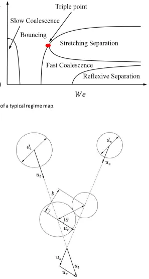
the droplets stretch and then separate due to the off-center collision), the reader is referred to FIG. 4

to distinguish between the collisions outcomes. These regimes are mapped in the parameter space of

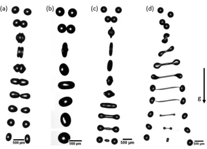
the impact parameter ( ) and Weber number ( ), as shown in FIG. 1. The impact parameter is the

normal distance ( ) from the center of one of the colliding droplets to the vector of the relative

velocity that is plotted from the center of the other droplet, normalized by the sum of the two droplets

radii,

(1)

as sketched in FIG. 2. Where, and Therefore, has a value

between 1 and 0, where 1 indicates a grazing collision and 0 a head-on collision. The Weber number

is the ratio of the kinetic energy, based on the relative velocity, to the droplet surface energy ,

(2)

and are the droplet fluid density and surface tension, respectively. and are the small droplet

3 FIG. 1. A schematic of a typical regime map.

FIG. 2. Schematic of the geometry of droplet collisions.

In FIG. 1 there are four transitional boundaries separating the five regimes: slow coalescence (i.e.,

between slow coalescence and bouncing regimes) , bouncing (i.e., between bouncing and fast

coalescence regimes below the triple point, and continues above the triple point between bouncing

and stretching separation regimes), stretching separation (i.e., between fast coalescence and

4

separation regimes).There were many attempts to model these different transitional boundaries.

Ashgriz and Poo (1990)studied the effect of the size ratio on water droplet collisions and derived two

models to evaluate the boundaries of stretching separation and of the reflexive separation. Although

the models consider the effect of the size ratio, they were for inviscid droplets. Later on, Jiang et al.

(1992) developed a model for the stretching separation boundary in which the viscosity effect was

explicitly involved in a form of two parameters. To the best knowledge of the authors, there has not

been a complete reflexive separation model considering the viscous dissipation. Nevertheless, Qian

and Law (1997) reported that the onset of the reflexive separation at head-on collision can be

correlated with Ohnesorge number ( ); where, is the dynamic viscosity of the droplet.

number is the ratio of the viscous energy to the surface energy. Gotaas et al. (2007b) used the

approach of Qian and Law (1997) to correlate the onset of the reflexive separation with a wide range

of viscosities (1-50 mPa s). Although Qian and Law (1997) and Gotaas et al. (2007b) were able to

correlate the onset of the reflexive separation to Oh number which allows consideration of the

viscosity effect, the size ratio of the colliding droplet was not considered. Tang et al. (2012) provided

a more detailed model for the onset of the reflexive separation taking into account both the effect of

viscosity and size ratio. The modelling of the slow coalescence boundary has received less attention

due to the difficulties of colliding droplets at very low . Bouncing modelling was conducted by

Estrade et al. (1999) who developed a model for the lower boundary of the bouncing regime based on

ethanol droplet collisions data at different size ratios. The model includes, a shape factor that can be

used as a parameter to fit the data.

Kuschel and Sommerfeld (2013) conducted extensive experimental work for solutions with different

solid content and thereby different viscosities to investigate the role of viscosity. The authors reported

that the stretching separation and the reflexive separation re gimes are shifted toward higher Weber

Numbers by increasing the viscosity. Therefore, the inviscid models of Ashgriz and Poo (1990) are not

adequate for high viscosity droplet collisions, while the Jiang et al. (1992) model was able to predict

the boundary of the stretching separation region by adapting the viscous loss parameters in the model

to fit the experimental data. Sommerfeld and Kuschel (2016) further extended the study of Kuschel

and Sommerfeld (2013) by conducting more experiments on pure liquids. The authors were able to

correlate the critical of the onset of the reflexive separation (at ) for different viscosities with

the Capillary number, which is the ratio of the viscous forces to the surface tension forces (

.The difference between the value of the onset of reflexive separation of water and this critical is then used to shift the boundary curve from the model of Ashgriz and Poo (1990) toward

higher . This approach successfully predicted the transitional boundary of reflexive separation

5

stretching separation boundary and mentioned that the adapted values of the two parameters in this

model can be correlated with a normalized relaxation velocity ( ).

On the other hand, the modelling of the lower boundary of the bouncing regime has received less

attention in comparison with the modelling of the other boundaries. Sommerfeld and Kuschel (2016);

Kuschel and Sommerfeld (2013); Sommerfeld and Lain (2017) reported that the model of Estrade et

al. (1999) can reasonably predict the lower boundary of the bouncing regime above the triple point

by adapting the shape factor to let the curve fit the experimental data. However, the model fails to

predict the boundaries below the triple point. The only attempt to modify this model was by Hu et al.

(2017) who altered the considered kinetic energy, which will be explained later in section IV, and

added a viscous loss term. However, the performance of this model was only validated against

simulation data of alumina droplets

In this paper, new experimental regime maps of binary droplet collisions of 2%, 4%, and 8% HPMC will

be reported to examine the effect of the viscosity. The collisions are restricted to identical droplets

size at room conditions. The three different concentrations have different viscosities, so this paper

shows the effect of the viscosity on the regime maps. In addition, the modelling of bouncing regime

will be discussed in detail. This will be through examining the performance of the existing models and

defining the neglected physics that undermine the performance of the models. Finally, we propose a

modified model to predict the boundary of the bouncing regime. It should be noted that, the models

of the other regime boundaries are not considered in this study as the aim of this paper is to shed the

light on the bouncing regime.

II.

THEORY OF BOUNCING

In this section, the theory of bouncing will be explored based on what have been reported in the

previous studies of binary droplets collisions. The theory provides a simple background, about

bouncing phenomenon of binary droplets collisions, which helps to understand the logic behind the

assumptions of bouncing modelling that will be explained in sections IV and V.

The phenomenon of droplet bouncing has been widely studied expe rimentally and numerically.

Bouncing occurs at a critical impact kinetic energy range, above and below which merging occurs (Qian

and Law, 1997; Tang et al., 2012). This is widely attributed to the presence of an air layer between the

two colliding droplets (Orme, 1997). At low impact velocity the air has sufficient time to be discharged.

However, if the velocity is increased the air will be trapped between the two droplets and hence the

droplets deform. A flattened interface will be formed between the two droplets, which causes

6

of the impact kinetic energy by the deformation of the droplets, as it will be converted into surface

energy and internal flow that relaxes later by the effect of the viscous dissipation. Once the impact

kinetic energy vanished, bouncing occurs by the action of the surface tension which tends to recover

the spherical shape to minimize the surface energy. Further increasing the impact velocity forces the

air layer to be discharged and rupture the interface and therefore merging with large deformation

would occur (fast coalescence).

Apart from the impact velocity, the bouncing regime was found to depend on the material of the

droplets and the surrounding gas. For example, at atmospheric pressure hydrocarbon droplets show

bouncing at the entire range of the impact parameter, whilst water shows bouncing only at high values

of impact parameter. In addition, milk droplets show no bouncing at the entire range of impact

parameter (Finotello et al., 2018). The merging of two droplets was attributed to van der Waals forces

(Zhang and Law, 2011; Pan et al., 2008). However, the thickness of the air layer between the colliding

droplets should be small enough for the van der Walls forces to be effective. Therefore, the difference

in the bouncing observation could be more related to the difference in molecular dynamics at the

surface of the droplets of different liquids. In addition, changing the conditions of the surrounding gas

shows a noticeable effect on the collision outcome (Krishnan and Loth, 2015; Qian and Law, 1997).

Increasing the gas pressure, density or molecular weight would promote the bouncing regime.

However the presence of the droplet s liquid vapor in the surrounding gas would promote the

coalescence regime (Qian and Law, 1997). All that makes it difficult to define a bouncing criteria that

is allows to distinguish between bouncing and coalescence based on the impact details such as

and .

III.

EXPERIMENTAL METHODS

The apparatus

The experimental setup is illustrated in FIG. 3. It consists of two custom-made monodisperse nozzles,

two high pressure syringe pumps, a high-speed camera (Photron mini AX100), a camera

(acA1300-200um - Basler ace), two strobe lights, two function generators, a pulse generator and two amplifiers.

The fluid is driven by the syringe pumps to the nozzles to create a continuous jet. Two square wave

signals are programmed in the function generator and sent via 20X amplifier (PiezoDrive PDu150CL)

to a piezo chip that is built into the nozzle. The piezo provides the required vibration to excite the jet

and hence break it up into a reproducible droplet stream. By directing the nozzles towards each other

7

collide. The bases of the nozzles posts have XYZR micro traversers, which all ow the alignment of the

droplet streams to be collided in the same plane. The side industrial camera that is attached to a

microscopic lens is used to make sure that droplet streams collide in the same plane. The maximum

frame rate of this camera is 200 fps; therefore, it is used with a strobe illumination source in order to

freeze the movement of the droplet streams. This is done by synchronizing the pulse generator, which

controls the strobe light, with one of the nozzles via the function generator. The collision outcome is

recorded using the high-speed camera at 30000 fps, which allows 256 x 384 pixel in the Field of View

(FOV). The high-speed camera is synchronized with another strobe light via the other function

generator. This puts more control on the exposure time as the strobe light can provide 10 ns pulse

duration. However, images with less light reflection were obtained at 3 of light pulse duration.

The high-speed camera was attached to a Navitar microscopic zoom lens by which magnification can

be controlled. However, although we can decrease the number of microns per pixel by zoo ming in,

this would reduce the FOV. A pixel was selected as balance between resolution and FOV for

the droplet size in this study. Based on this resolution, the measurement of the droplet size has an

uncertainty of 4%.

I ID This dispensing tip

size produces droplets diameter of 360- flow rate and the physical

properties of the fluid; data on droplets size variation due to frequency change are provided in the

Supplemental Material. The flow rate range used is 2.5-6 ml/min. The applied frequency in the nozzles

ranged from 1.5-1.85 KHz depending on the jet flow rate and the physical properties. The impact

parameter was controlled by using the aliasing method of Gotaas et al. (2007a). This was done by

applying a frequency shift of 3 Hz, between the two nozzles, which leads to periodically sweeping the

impact parameter between 1 and 0. The number is varied by changing the angle between the two

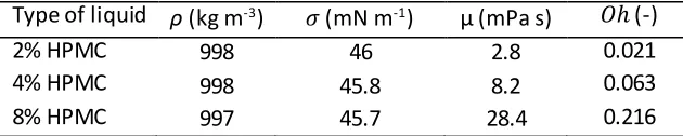
streams as wider angle produces higher relative velocity ) and hence higher . Four regimes

were produced in this study, bouncing, fast coalescence, reflexive separation and stretching

separation as shown in FIG. 4. The slow coalescence regime was not considered in this study due to

8 FIG. 3. Droplet collisions rig.

FIG. 4. Four different collisions outcomes of 2% HPMC droplets collisions, bouncing (a), fast coalescence (b), reflexive separation (c) and stretching separation (d).

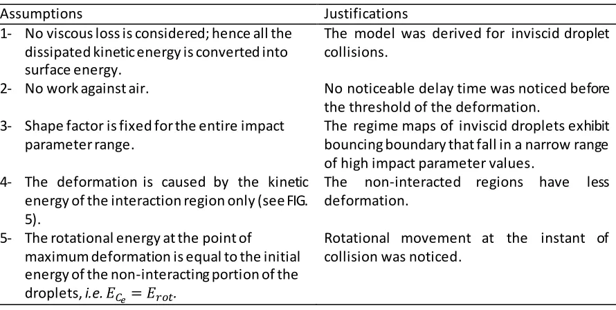
Droplet fluids

Three different concentrations, 2%, 4%, and 8%, of Hydroxypropyl Methylcellulose grade 603

Shin-Etsu Chemical's PHARMACOAT® (HPMC) solutions, in deionised water, were used for this study. The

viscosities of the solutions were measured in a Rheometer (Bohlin Gemini) by using a cone and plate

geometry and shear rate range from 1 to 270 . The solutions exhibit a Newtonian behaviour within

9

tensiometer (KSV CAM 200). The density was measured by weighting 50 ml of the solution using an

analytical balance. Table I illustrates the physical properties of the three solutions. The measured

values agree with the values that have been reported in the literature (Parker et al., 1991; Kokubo and

Obara, 2008). All collisions experiments and measurements carried at atmospheric conditions and

room temperature 20 °

TABLE I. Physical properties of the three HPMC systems that are used in this work.

Type of liquid (kg m-3_{) (mN m}-1₎ P _(-)

2% HPMC 998 46 2.8 0.021

4% HPMC 998 45.8 8.2 0.063

8% HPMC 997 45.7 28.4 0.216

Tracking methodology

A tracking algorithm was developed to obtain the impact details from the recorded videos. the

tracking algorithm is implemented by using a MATLAB based tracking software, called Droplet

Morphometry and Velocimetry (DMV) that was developed by Basu (2013), to track droplets before

the collision point. For each droplet, DMV provides the XY positions of droplet center, XY velocities,

equivalent diameter, time, frame number, and droplet ID (as a number). Based on this data provided

by DMV, the impact details are then extended with very small increments to the exact collision point

using a MATLAB code that was developed by the author. The impact parameter and are then

evaluated at the collision point. The advantage of this method is to avoid cases when the exact

collision point does not appear in the recording (i.e. occurred in an instance between two consequent

frames), especially at high . It should be noted that the use of the MATLAB code alongside with

DMV is essential, because the latter is not designed to estimate the impact parameter. More details

on the tracking methodology can be found in Appendix A.

IV.

CURRENT MODELS FOR THE BOUNCING REGIME BOUNDARY

Estrade et al. (1999) model for the bouncing regime boundary is based on an energy criterion. It states

that bouncing occurs if the component of kinetic energy that contributes to the deformation of the

droplets is less than the increase in surface energy required to reach the limit of maximum

10

assumed to occur. A number of assumptions are made to derive this criterion and the subsequent

equation for the boundary, these are detailed in Table II.

Applying the assumptions 1 and 2 in Table II an energy balance can be written between the system

energy just prior to collision and at the point of maximum deformation

. (3)

Where, is the part of the droplet kinetic energy that does not contribute to the deformation,

is the kinetic energy that contributes to the deformation, is surface energy of the droplets before

the collision, is surface energy of the droplets at the maximum deformation, and is the

rotational kinetic energy.

TABLE II. Assumptions that Estrade et al. (1999) made to develop the bouncing model.

Assumptions Justifications

1- No viscous loss is considered; hence all the dissipated kinetic energy is converted into surface energy.

The model was derived for inviscid droplet collisions.

2- No work against air. No noticeable delay time was noticed before

the threshold of the deformation. 3- Shape factor is fixed for the entire impact

parameter range.

The regime maps of inviscid droplets exhibit bouncing boundary that fall in a narrow range of high impact parameter values.

4- The deformation is caused by the kinetic energy of the interaction region only (see FIG. 5).

The non-interacted regions have less deformation.

5- The rotational energy at the point of

maximum deformation is equal to the initial energy of the non-interacting portion of the droplets, i.e. .

Rotational movement at the instant of collision was noticed.

Applying assumption 4, the kinetic energy that contributes to the deformation is that of the interacting

volumes shown in FIG. 5 and is given by

cos (4)

Where is the volume of the interaction region, which is given by

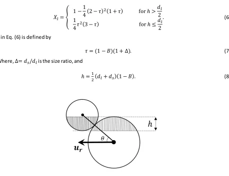
(5)

Where is the ratio of the interaction region volume, of the large droplet, to the total droplet

11

for

for

(6)

in Eq. (6) is defined by

. (7)

Where, is the size ratio, and

. (8)

FIG. 5. A schematic representation of the interaction regions (in grey).

The surface energy of a droplet is the production of the surface tension and the droplet surface area.

Thus, the total surface energy of the droplets before the collision is given by

. (9)

The droplets reach the maximum deformation limit just before bouncing separation, i.e. when the

kinetic energy of the interaction regions (Eq. (4)) is completely converted into surface energy

(assumptions 1 and 2). Estrade et al. (1999) described the surface energy at the maximum

deformation by

(10)

Where, is a shape factor that is given by

12

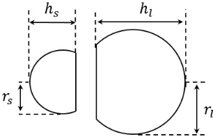
Estrade et al. (1999) reported that in case of collisions between unequal size droplets the shape

factor can be either calculated based on the small droplets, or it can be based on the

large droplet, , see FIG. 6.

FIG. 6. Droplet shape at the instance of maximum deformation according to Estrade et al. (1999).

Substituting Eq. (4), Eq. (9), and Eq. (10), in Eq. (3) and applying assumption 5 with rearrangement

gives

(12)

which is the critical that describe the boundary of the bouncing regime as a function of .

Hu et al. (2017) extended the model of Estrade et al. (1999) to higher viscosity systems, by considering

the viscous dissipation within the droplet . Thus, the energy balance becomes

(13)

The viscous dissipation was considered a fixed percentage (independent of ) of the kinetic energy

that contributes to the deformation. Thus, Eq. (13) becomes

. ₍₁₄₎

Moreover, Hu et al. (2017) used a different approach in defining the kinetic energy that contributes

to the deformation, as given by

cos cos (15)

Where, and Importantly, Eq. (15) considers the entire

13

Substituting Eq. (15), Eq. (9), and Eq. (10), in Eq. (14) , as well as applying assumption 5, gives the

model of Hu et al. (2017), which predicts the critical of the lower boundary of the bouncing

regime as a function of :

(16)

It should be noted that Estrade et al. (1999) and Hu et al. (2017) have different definition to the kinetic

energy that contributes to the deformation at head-on collisions (i.e. where both models use the

entire mass of the droplets in ) Eq. (4) and Eq. (15), respectively. As Estrade et al. (1999) approach

assumes one droplet is not moving while the other approaching at the relative velocity . Whereas, Hu

et al. (2017) considers the movement of both droplets. This will be investigated in further details in

section V.B.1.a.

V.

RESULTS AND DISCUSSION

A.

HPMC regime maps

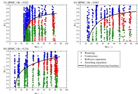
The regime maps of 2% HPMC, 4% HPMC, and 8% HPMC are shown in FIG. 7. The expect regimes were

seen and their overall shapes are consistent with previous work, for instance (Qian and Law, 1997;

Kuschel and Sommerfeld, 2013). The Figures clearly show that the reflexive separation boundary is

shifted toward higher by increasing the viscosity. The reflexive separation regime disappeared at

8% HPMC for the investigated range of . That qualitative trend of the viscosity effect agrees with

the previous studies of Kuschel and Sommerfeld (2013); Sommerfeld and Kuschel (2016); Gotaas et

al. (2007b); Finotello et al. (2018); Finotello et al. (2017), where more details about these trends can

be found.

The regime maps also show that as the viscosity increases the bouncing regime boundary shifts toward

lower . This might be because at higher viscosity, more kinetic energy is viscously dissipated and

hence less energy is converted into surface energy. This results in less deformation and consequently

less trapped air between the droplets which can be easily discharged to promote the coalescence

regime.

In the following sections, the modelling of the bouncing boundary will be discussed by assessing the

existing models and proposing a new model. In FIG. 7 the solid black curve is fitted manually to the

bouncing boundaries of the three HPMC systems. This curve will be used as reference in the oncoming

discussion to allow for removing the data points and reducing the noise in the Figures. It should be

14

FIG. 7. HPMC regime maps for the three concentrations 2%, 4%, and 8%.

B.

Assessment of the existing bouncing models

To assess the performance of the models of Estrade et al. (1999) and Hu et al. (2017) a line defining

the boundary of the bouncing regime was manually fitted to the experimental data, see FIG. 7. This

curve was digitized using Origin 2017 with a increment of 0.01. These data points were used to

optimize the shape factor by minimizing the Mean Absolute Error:

MAE (17)

The use of the MAE quantitatively characterizes the performance of the models. The viscous

dissipation parameter in Hu et al. (2017) model was set as 0.5 for the three HPMC solutions. This

value was used as an approximation based on the numerical simulation of Xia and Hu (2014) who

reported that the viscous loss of alumina droplets that has viscosity 14 mPa.s is approximately 50%

of the kinetic energy.

FIG. 8 clearly reveals that the models of Estrade et al. (1999) and Hu et al. (2017) are not adequate to

predict the boundary of bouncing regime for all range of . However, plotting them with different

viscosities would be helpful to theoretically analyzing their limitations, as will be shown in the

following discussion.

0 10 20 30 40 50 60 70 80 90 100 0.0 0.1 0.2 0.3 0.4 0.5 0.6 0.7 0.8 0.9 1.0

0 10 20 30 40 50 60 70 80 90 100 0.0 0.1 0.2 0.3 0.4 0.5 0.6 0.7 0.8 0.9 1.0

0 10 20 30 40 50 60 70 80 90 100 0.0 0.1 0.2 0.3 0.4 0.5 0.6 0.7 0.8 0.9 1.0 B [ - ]

We [ - ]

2% HPMC, Oh = 0.021

B

[ -

]

We [ - ]

4% HPMC,Oh = 0.063

Bouncing Coalescence Reflexive separation Stretching separation

Experimental bouncing boundary

B

[

-

]

We [ - ]

15

FIG. 8. The performance of Estrade et al. (1999) model in Eq. (12) and Hu et al. (2017) model in Eq. (16) on the HPMC regime mapes for the three concentrations that used in this work, 2%, 4%, and 8%.

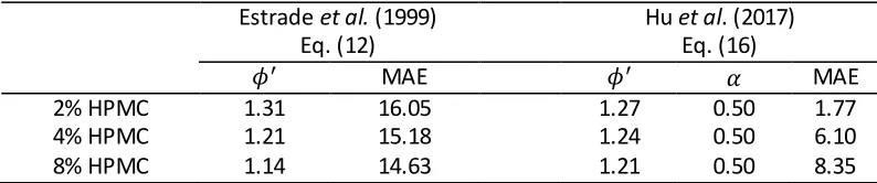
TABLE III. A quantitative summery of the performace of the models of Estrade et al. (1999) and Hu et al. (2017).

Estrade et al. (1999) Eq. (12)

Hu et al. (2017) Eq. (16)

MAE MAE

2% HPMC 1.31 16.05 1.27 0.50 1.77

4% HPMC 1.21 15.18 1.24 0.50 6.10

8% HPMC 1.14 14.63 1.21 0.50 8.35

Table III, shows an overall improvement in the prediction when Hu et al. (2017) model is used where

the MAE remains in the range of 1.74 to 8.35 for the three systems, whereas, Estrade et al. (1999)

model shows MAEs in the range of 14.63 to 16.05. It can also be noticed from Table III and FIG. 8 that

Estrade et al. (1999) model shows an increasing accuracy as the viscosity increases, as the MAE was

reduced from 16.05 in 2% HPMC to 14.63 in 8% HPMC. In contrast, Hu et al. (2017) model exhibits an

opposite behavior, where the MAE increased from 1.74 in 2% HPMC to 8.35 in 8% HPMC, respectively.

Moreover, qualitatively, for the three systems the model of Estrade et al. (1999) could not follow the

0 20 40 60 80 100 120 140 0.0 0.1 0.2 0.3 0.4 0.5 0.6 0.7 0.8 0.9 1.0

0 20 40 60 80 100 120 140 160 180 0.0 0.1 0.2 0.3 0.4 0.5 0.6 0.7 0.8 0.9 1.0

0 20 40 60 80 100 120 140 160 180 200 0.0 0.1 0.2 0.3 0.4 0.5 0.6 0.7 0.8 0.9 1.0 B [ - ]

We [ - ] 2% HPMC, Oh = 0.021

B

[ -

]

We [ - ] 4% HPMC,Oh = 0.063

Estrade et al. (1999) Hu et al. (2017)

Experimental bouncing boundary

B

[

-

]

We [ - ]

16

trend of the experimental boundary starting from under-prediction of at low and crosses the

experimental curve above the triple point to over-prediction of at high . However, the boundary

predicted by the model of Hu et al. (2017) crosses the experimentally observed boundary near the

triple point, especially in the cases of 4% and 8% HPMC, by over-predicting at low and

under-predicting at high . The following paragraphs explain the reasons behind these observations.

In both models it is assumed that the maximum deformation limit is independent of the impact

parameter (i.e. constant shape factor, assumption 3 in Table II). However, the maximum deformation

limit decreases significantly as the impact parameter increases, as can be seen in case of 2% HPMC in

FIG. 9. Consequently, an over-prediction of would be expected at high values if the model is

fitted to the experimental at =0, as shown in FIG. 10. This explains the trend of the model of

Estrade et al. (1999) in FIG. 8, as the minimum MAE fits the model at a value near the triple point

(the cross point). This means the selected value produces less surface area at the maximum

deformation limit than that at near head-on collisions and thereby under-prediction of below the

cross point and higher than that at high values above the cross point which cause the

over-prediction of .

However, Hu et al. (2017)et al. (2017) shows an under-prediction of at high values of when the

model fits the experimental boundary at =0, as shown in FIG. 10. This trend is contrary to

expectations due to the constant shape factor assumption. This can be explained by the

overestimation of kinetic energy, at high values, that is considered by using of the entire droplet

mass regardless the percentage of interaction regions. The excessive kinetic energy that is considered

to contribute to the deformation has an opposite effect to the constant shape factor assumption. This

opposite effect reduces the impact of these assumptions on the model, which explains the overall

improvement in the prediction of the model of Hu et al. (2017) compared to the model of Estrade et

al. (1999). However, the excessive kinetic energy seems to have a larger impact on the curve than

that of the constant shape factor assumption. This leads to an under prediction of at high

values when the model is fitted to the experiments at head-on collisions, as shown in FIG. 10. That

explains the trend of the model of Hu et al. (2017) in FIG. 8, as the Minimum MAE selects value

that fits the model at a cross point near the triple point and thereby an under-prediction of above

this point and an over-prediction of below it.

The case of 8% HPMC in FIG. 9 shows that at high viscosity, the assumption of constant shape factor

has less significance in comparison to the case of 2% HPMC. This because that the bouncing boundary

occur at low and hence at low kinetic energy. Due to the high viscosity, significant amount of this

17

energy and hence low deformation occurs at low , which makes the shape factor more comparable

with that at higher values in comparison to the bouncing of lower viscosity droplets. Therefore, the

prediction accuracy increases with the increase of the viscosity by using the model of Estrade et al.

(1999). However, the accuracy of the model of Hu et al. (2017) decreases by increasing the viscosity

as the opposite effect of the constant shape factor to the effect of the excessive kinetic energy is lower

than that at low viscosity.

Although Estrade et al. (1999) and Hu et al. (2017) have different definition to the kinetic energy that

contributes to the deformation at head-on collisions, this should not affect the above discussion as

both models are optimized by fitting the shape factor for the minimum MAE. This means any

difference due to the difference in the kinetic energy will be recovered by the fitted shape factor.

Similarly, the existence of the viscos loss term in the model of Hu et al. (2017) should not affect the

discussion. Ultimately, the difference in the shape of the two models is due that Estrade et al. (1999)

consider the mass of the interaction regions in the kinetic energy that contributes to the deformation

while Hu et al. (2017) consider the entire mass; this cannot be recovered by the fitted shape factor

because X is a function of B while the shape factor is not.

From the discussion in this section, an accurate model that can evaluate the boundary of the bouncing

regime requires, a shape factor that accurately reflexes the geometry of the droplet at maximum

deformation, correct definition of the kinetic energy that contribute s to the deformation, good

estimation to the viscous losses, and implementing the effect of the impact parameter on the shape

factor and the kinetic energy that contributes to the deformation. Therefore, in the next sections,

these parameters will be assessed firstly at head-on collisions then the analysis will be extended to

18

FIG. 9. The maximum deformation of 2%and 8% HPMC at differenet values of impact parameter for Weber numbers that occur on the boundary of the bouncing regime.

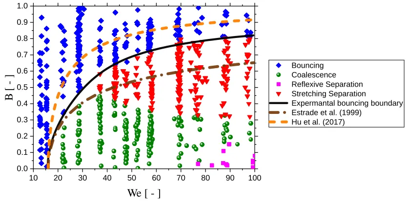
FIG. 10. The performance of the existing models when they are fitted to the onset of coalescence at head-on collisions, which show the over-prediction of the model of Estrade et al. (1999), Eq. (12), and the under-prediction of the model of Hu et al. (2017), Eq. (16) on 4% HPMC regime mape. is 5.0 in the model of Estrade et al. (1999) while it is 3.5 in the model of Hu et al. (2017) and is 0.5.

A

head-on collisions

a. Kinetic energy assessment

10 20 30 40 50 60 70 80 90 100 0.0

0.1 0.2 0.3 0.4 0.5 0.6 0.7 0.8 0.9 1.0

Bouncing Coalescence Reflexive Separation Stretching Separation

Expermantal bouncing boundary Estrade et al. (1999)

Hu et al. (2017)

B

[ -

]

19

As mentioned earlier, the two models have different definition to the kinetic energy that contributes

to the deformation. To assess the validity of these two different approaches, they are examined for

head-on collisions, where both approaches consider the kinetic energy of the total drop mass.

The momentum of a moving droplet is given by , where and are mass and velocity of the droplet respectively. Therefore, the kinetic energy of the droplet is given by:

(18)

This relation will show if the two approaches of the kinetic energy are conserve the momentum in a

zero-momentum frame.

In head on bouncing collision of equal diameter ( ) droplets, if each droplet has a velocity equal to

, the total momentum of the two colliding droplets is

(19)

Substituting Eq. (19) in Eq. (18) gives the total kinetic energy of the droplets

(20)

At head on collisions, and cos are both equal one. Thus, the kinetic energy of the model of Estrade et al. (1999), from the combination of Eqs. (4-6), is . This reveals that

Estrade et al. (1999) double the kinetic energy that contributes to the deformation by compared to

Eq. (20). However, the approach of Hu et al. (2017) more universal, as simplifying Eq. (15), for

head-on collisihead-ons of equal size droplets, gives , which recovers Eq. (20). Thus, the

approach of Hu et al. (2017) will be the considered in the rest of this paper.

b. Shape factor assessment

By looking at the both aforementioned models (Eq. (12) and Eq. (16)) it can be realized that the shape

factor should always have a value >1, otherwise the models would produce zero or negative values

of . This implies that must have a value that is always less than 0.40, according to Eq. (11), as

shown in FIG. 11. However, 2 for grazing collisions ( =1), and the direct measurement at

head-on collisihead-on from the images of 2% HPMC in FIG. 9 at maximum deformatihead-on reveals that 0.648

for 2% HPMC. This range of (from 2 to 0.648) is above 0.4, which implies that the shape factor

<1, as shown in FIG. 11. Thus, this shows that the commonly used shape factors of the existing models

are not seen in reality, and hence the suggested equation for the maximum deformation seems to be

invalid. To verify the validity of this equation, the shape factor of spherical cup was rederived in this

work, see Appendix B. The new derivation of the shape factor proved that Eq. (11) should be in the

20

(21)

and the form of Eq. (11) is might be due to a derivation mistake by Estrade et al. (1999). Eq. (21) shows

that >1 for the visible range of (from 0 to 2), as shown in FIG. 11.

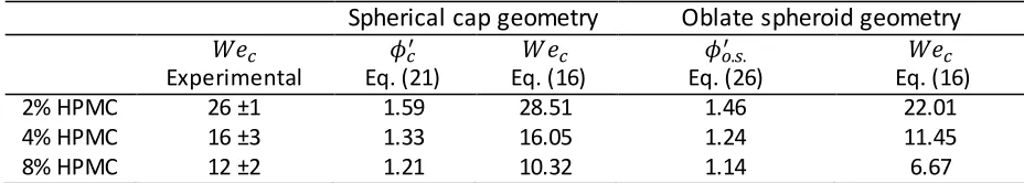
As the shape factor was corrected in Eq. (21), it would be interesting to use it, by measuring from

the experimental images, to evaluate the critical of the onset of coalescence at head-on

collisions. This by using the model of Hu et al. (2017) as it implements the correct kinetic energy as

justified in the previous section. The model firstly tested without considering the viscous losses (i.e.

). The model slightly over-predicts the onset of coalescence in case of 2% HPMC and gives a

reasonable agreement in 4% HPMC and 8% HPMC, as illustrated in Table IV. However, adding viscous

losses would further over-estimates . This implies that the spherical cup geometry over-estimates

the surface energy at the maximum deformation. Thus, there is a requirement for a shape factor that

has a better agreement with the geometry of the droplets at the maximum deformation. Thus, a new

shape factor will be proposed, in the next sub-section.

TABLE IV. Comparison between the experimental and the predicted of the onset of coalescence using Eq. (16) using different shape factors (spherical cup and oblate spheroid) at , and .

Spherical cap geometry

Oblate spheroid geometry

Experimental Eq. (21) Eq. (16) Eq. (26) Eq. (16)

2% HPMC 26 ±1 1.59 28.51 1.46 22.01

4% HPMC 16 ±3 1.33 16.05 1.24 11.45

21

FIG. 11. The shape factor in Eq. (11) and Eq. (21) as a function of the shape parameter .

c. The proposed shape factors

The images in FIG. 9 reveals that the maximum deformation of the droplets at head-on collisions have

a shape that approximates an oblate spheroid more than spherical cup. The surface area of an oblate

spheroid is given by

ln

(22)

Where, and are shown in FIG. 12, and . Thus, the surface energy equation at the

maximum deformation can be given by

ln

ln

(23)

which considers the effect of size ratio by implementing

and

and . It should be noted that and are expected to be unequal in case of

collisions between droplets that have non-identical size. This is due to the difference in the capillary

pressure ( ) between the droplets, as the small droplet has higher capillary pressure and hence

higher resistance to the deformation. This is in contrary to the assumption of Estrade et al. (1999)

that .

0.0 0.2 0.4 0.6 0.8 1.0 1.2 1.4 1.6 1.8 2.0 0

1 2 3 4 5

Corrected shape factor



'

Estrade et al. (1990) shape factor



'

Sha

pe

f

ac

tor

[ - ]

22

FIG. 12. The oblate spheroid shape that proposed for the maximum deformation at head-on collisions.

From mass conservation before the collision and at the maximum deformation, the volume of the

oblate spheroid, given by , is equal to a volume of a sphere, given by

, that has a diameter equal to the droplet diameter before the collision.

(24)

Solving Eq. (24) for , , and and substituting it in Eq. (23) gives

ln

ln

(25)

From the analogy between Eq. (25) and Eq. (10), the shape factor of an oblate spheroid geometry

( ) is given by

ln

ln

23

Using the new shape factor of the oblate spheroid, Eq. (26), rather than the shape factor of the

spherical cap, Eq. (21), with keeping , results in an under-prediction of for the three HPMC

solutions, as shown in Table IV, which is the expected scenario due to the neglect of the viscous losses.

This reveals that the oblate spheroid geometry is better in describing the geometry of the droplet at

the maximum deformation, since its produce shape factor that have less value than the spherical cup,

as illustrated in Table IV, and hence lower surface energy at the maximum deformation.

d. Viscous losses estimation

The process of bouncing can be divided into two stages: the initial deformation from the time of

contact, , to the point of maximum deformation, , and a period of oscillating relaxation where

the droplets return to their original spherical shape at , as shown in FIG. 13. The total viscous

dissipation in the bouncing collision process takes place during both these periods due to the induced

internal flow. Assuming viscous losses are the only sources of energy loss, then the viscous energy

loss, , is equal to the difference in the system kinetic energy before and after the head on collision,

i.e. . Where, is the kinetic energy of the droplets a post collision is given by

and where is the velocity of each of the rebounding droplets. This velocity can be measured by

tracking the separating droplets.

The viscous loss in the bouncing model, is that due to the deformation in the period from to . Therefore, to estimate it is necessary to estimate the ratio of the viscous losses during period of

- to the total viscous losses, . If the droplets are viscous and recovered their spherical shape

without oscillation, this fraction will be 50% and hence . This is based on the

assumption that the losses during the compression period from to , is equal relaxation period

when the droplet returns to its spherical shape at . In the more general case when the droplets

show oscillations during the relaxation period, see FIG. 14, estimating requires an estimate of the

24 FIG. 13. The stages of bouncing process.

FIG. 14. The radial oscillation of the droplets during the bouncing collision.

If the assumption is made that the viscous energy loss in each overshoot is proportional to the

elongation of the droplet,

,

to the total viscous losses can be approximated by

.

Where, is the length of the droplet measure along it principal axis. However, the viscous loss that

considered in the bouncing model is roughly half the viscous loss in the period . Thus, the

viscous losses factor is in the order of

t r n t

r n-1

t r4 t

r3

t_r2

t r1

t m n-1

t m n t

m4 t

m3

t m2 t

m1 _{Oscillation of the radial diameter}

Non deformed droplet diameter

Radia

l exp

an

tion

Time

25

.

8% HPMC shows that 88% of is dissipated by the total viscous losses, and no oscillation after ,

which means 44%, as shown in Table V. While, 4% HPMC shows 70% of is dissipated by the

total viscous losses, and of one cycle after (i.e. reaches its final relaxation state at ). More

oscillations were noticed in 2% HPMC, which shows six cycles after ; and 75% of is dissipated

by the total viscous losses. Applying Eq. (28) to 2% HPMC and 4% HPMC gives that the viscous

dissipation factor is approximately 0.11 and 0.33, respectively, as shown in Table V. Using these

approximated values of in the model of Hu et al. (2017) with the measured values of the proposed

shape factor Eq. (26), shows good agreement of the predicted with the experiments, as shown

in Table V.

TABLE V. Comparison, at head-on collisions, between the experimental and the predicted of the onset of coalescence using Eq. (16) with the oblate spheroid shape factor, Eq. (26), and Eq. (28) for the viscous dissipation factor.

Eq. (28) Eq. (26) experimental Eq. (16)

2% HPMC 0.11 1.46 26 ±1 24.72

4% HPMC 0.23 1.24 16 ±3 15.8

8% HPMC 0.44 1.14 12 ±2 11.90

The effect of the impact parameter

a. Kinetic energy assessment

As mentioned early, considering the total mass of the droplet in leads to under-predict at

high values of . Therefore, the mass of the interaction regions should be considered in the approach of Hu et al. (2017) in evaluating the kinetic energy that contributes to the deformation. This should be

considered for both small and large droplet, in case of collisions of unequal size droplets. Therefore,

the equation of the kinetic energy that contributes to the deformation will be

l s cos s s cos (29)

Where, is given by Eq. (6) and

for

for

26

Where, and are defined in Eq. (7) and Eq. (8), respectively.

b. Shape factor assessment

As mentioned before the degree of deformation decreases with the impact parameter (i.e. decrease

in the surface area at the maximum deformation), see FIG. 9. Therefore, to predict the lower boundary

of the bouncing regime, for the entire range of B, the decrease in the surface area of the droplet at

the maximum deformation needs to be considered. In FIG. 9, it can be noticed that the deformation

has less dependency on the impact parameter at the range from 0 to 0.3 than at the range from 0.3

to 0.7, especially in case of 2% HPMC. Thus, we need to account for the non-linear decrease in shape

factor see with increasing . As the factor e is an indicator of deformation, the surface area can be

correlated with via and the following power law correlation is proposed

. (31)

Where, , and are positive constants that can be optimized to fit the data. Therefore, is the

new shape factor that account for the effect of which is similar to that in Eq. (26) but using

instead of . Eq. (31) allows for that at , and hence .

c. The performance of the new model

Using Eq. (29) and the proposed shape factor , the bouncing boundary model will be

(32)

Using this model, Eq. (32), with the approximated values of in section V.B.1.d., and the measured

values of at head-on collisions, in Table VI, and then Optimizing , and instantaneously for the

minimum MAE, show significant improvement in the prediction of the bouncing boundary, as shown

qualitatively in FIG. 15. The proposed model shows excellent agreement with experimental data

whether above or below the triple point for the three HPMC solutions. Quantitatively, Table VI shows

that the MAE of the proposed model is significantly reduced compare to that of the models of Estrade

et al. (1999) and Hu et al. (2017) in Table III. Compare to the model of Estrade et al. (1999), the MAE

was reduced by 99%, 97%, and 87% for 2% HPMC, 4% HPMC, and 8% HPMC, respectively. And

compare to the model of Hu et al. (2017), it was reduced by 87%, 93%, and 77% for 2% HPMC, 4%

27

TABLE VI. The performance of the proposed model in Eq. (32) in predicting the bouncing boundary of 2%. 4%, and 8% HPMC.

Eq. (28) (at ) MAE

2% HPMC 0.11 1.46 0.86 2.75 0.23

4% HPMC 0.23 1.24 1.05 3.93 0.40

8% HPMC 0.44 1.14 1.11 4.70 1.91

FIG. 15. The performance of the proposed model Eq. (32) compare to bouncing boundaries on the HPMC regime mapes for the three concentrations, 2%, 4%, and 8% .

VI.

CONCLUSION

In this work, three novel regime maps of binary droplet collisions outcomes for three different

concentrations of HPMC aqueous solution, 2%, 4%, and 8% were developed experimentally. Increasing

the concentration of HPMC, increases the solution viscosity, and shifts the boundary of the separation

regimes toward higher due to the higher viscous dissipation. In, contrast the bouncing regime

boundary shifted toward lower ; because, the higher viscous dissipation reduces the deformation

and hence faster air discharge between the colliding droplets.

0 20 40 60 80 100

0.0 0.1 0.2 0.3 0.4 0.5 0.6 0.7 0.8 0.9 1.0

0 20 40 60 80 100

0.0 0.1 0.2 0.3 0.4 0.5 0.6 0.7 0.8 0.9 1.0

0 20 40 60 80 100

0.0 0.1 0.2 0.3 0.4 0.5 0.6 0.7 0.8 0.9 1.0 B [ - ]

We [ - ]

2% HPMC, Oh = 0.021

B

[ -

]

We [ - ]

4% HPMC,Oh = 0.063

Bouncing Coalescence

Reflexive Separation Stretching Separation The proposed model

B

[

-

]

We [ - ]

28

The performance of the existing models predictions of the boundary of bouncing regime was assessed

against the experimental data using the mean absolute error as a quantitative measure. Generally,

the model of Hu et al. (2017) shows better accuracy than the model of Estrade et al. (1999). The poor

performance of the model of Estrade et al. (1999) is primarily attributed to the assumption that the

surface energy at the maximum deformation is independent of the impact parameter, i.e. constant

shape factor. However, for the more viscous system studied here the experimental images clearly

show that the deformation reduces significantly with the impact parameter and consequently a

constant shape factor cannot be assumed. H also assumes a constant shape factor

however the inclusion of the entire droplet kinetic energy in the energy balance, in contrast to Estrade

et al. (1999)who only include the interacting regions, counteracts this assumption and reduces the

deviation of the model from the experimental data. (The H

does not help improve the fit as it does not change the shape of the curve.)

Several errors in the derivation of the models were also identified. The derivation of the spherical cap

shape factor of Estrade et al. (1999), which was reapplied by Hu et al. (2017), was shown to contain

an error. However, an oblate spheroid geometry was found to give a better fit to the droplet shape

at maximum deformation for head-on collisions than the spherical cap. Therefore, the oblate spheroid

surface area was applied to derive a new shape factor. Additionally, it was found that, the definition

of the collisional kinetic energy in the model of Estrade et al. (1999) was not general and led to errors,

for example it doubles the kinetic energy in the case of head on collisions. The definition of Hu et al.

(2017) is universally applicable and conserves momentum

Using the proposed oblate spheroid shape factor, the kinetic energy definition of Hu et al. (2017) but

accounting only for the mass of the interaction regions, a modified model for the bouncing regime

boundary was proposed. The shape factor for head-on collisions was taken directly from

measurements, and the reduction in shape factor with increasing B fitted empirically using a power

law model. Viscous dissipation was also taken into account in the proposed model and for each

HPMC concentration, a viscous dissipation factor was estimated directly from the experimental

observations by analyzing the decay in the oscillations of bubble shape which occurs after each

collision.

The proposed model shows a great fit to the experimental results. For all three HPMC concentrations

the critical We number for head on collisions is well predicted and the fit to the boundary of the

bouncing regime is excellent for across the range of We numbers tested, whether above or below the

triple point. Quantitatively, the MAE was reduced an order of magnitude compare to the literature

29

T

outcomes, which is very important for many applications such as spray drying. To make a better use

from the model, more investigation is required to quantify the maximum deformation limit and to

avoid the need for the direct measurements of the shape factor. This might need a deep

understanding of the role of the intervening gas layer.

VII.

Supplemental material

Data on the droplet sphericity prior to the collisions, and about the droplet size variation due to the

change of the frequency is provided.

ACKNOWLEDGMENTS

The authors gratefully acknowledge the useful discussions and assistance of Prof Phil Threlfall -Holmes, Prof Nik

Kapur and Gurdev Bhogal from the University of Leeds . The work was supported by EPSRC project:

E D D F ion of Micro- F P F

(grant ref: EP/N025245/1) and the University of Leeds.

APPENDIX A: DROPLETS TRACKING METHODOLOGY

The tracking starts by uploading the high frame rate video into DMV. In DMV, the frames are cut for

the region before collision point, as shown in FIG. 16. From each frame, DMV evaluates time ( ),

diameter ( ), and position (x, y) for each droplet. Every droplet is given ID number to enable the

tracking of each droplet through different frames. From every two successive frames, DMV evaluates

the velocity in x and y direction for each droplet, details on DMV can be found in Basu (2013). These

data are saved in excel sheet, which is then loaded into MATLAB to extend the position of the droplets

to the collision point. The extension procedure is as follow:

1. The (x, y) position of the tracked droplets in frame 4 in

FIG. 16

increment of time ( to become (x + , y + ). The increment of the time that

selected in this study is

2. The time will be updated by adding to the time of the last frame that the tracked droplet

appeared in, frame 4 in the example in FIG. 16.

3. When the newly calculated (x, y) positions of droplets and

satisfy at , the impact

30

The angle is a function of (x, y) positions of droplets and and can be estimated using the

following procedure considering that the frame of reference on the center of the droplet in FIG.

16:

1. Estimating the angle between the two streams of droplets ( and ) by using

tan tan .

2. Estimating the angle between the x axis and the line that cross the centers of the colliding

droplets and at the collision point using tan .

3. Estimating the relative velocity using cos .

4. Estimating the angle between the relative velocity vector and stream using

sin sin

5. The angle is estimated using tan .

FIG. 16. Tracking methodology to estimate the collision point and hence the impact parameter.

APPENDIX B:

SPHERICAL CUP SHAPE FACTOR DERIVATION

The volume of a spherical cup is

31

Where, is the radius of the deformed droplet (spherical cup), and is defined in FIG. 16. From the

mass conservation, Eq. (B1) will be equal to sphere volume, hence

(B2)

where, is the diameter of the non-deformed droplet. The surface area of the spherical cup is given

by

. (B3)

Substituting Eq. (B2) in Eq. (B3) and evaluating for the surface energy of colliding droplets at maximum

deformation give

(B4)

From mass conservation and substituting ,

(B5)

Sub (B5) in (B4) gives

. (B6)

From the analogy between Eq. (B6) and Eq. (10), the correct shape factor of spherical cup is

. (B7)

REFERENCES

Ashgriz, N. and Poo, J. 1990. Coalescence and separation in binary collisions of liquid drops. Journal of Fluid Mechanics.221, pp.183-204.

Basu, A.S. 2013. Droplet morphometry and velocimetry (DMV): a video processing software for time-resolved, label-free tracking of droplet parameters. Lab on a Chip.13(10), pp.1892-1901. Estrade, J.-P., Carentz, H., Lavergne, G. and Biscos, Y. 1999. Experi mental investigation of dynamic

binary collision of ethanol droplets a model for droplet coalescence and bouncing. International Journal of Heat and Fluid Flow.20(5), pp.486-491.

Finotello, G., Kooiman, R.F., Padding, J.T., Buist, K.A., Jongsma, A., Innin gs, F. and Kuipers, J. 2018. The dynamics of milk droplet droplet collisions. Experiments in Fluids.59(1), p17. Finotello, G., Padding, J.T., Deen, N.G., Jongsma, A., Innings, F. and Kuipers, J. 2017. Effect of

viscosity on droplet-droplet collisional interaction. Physics of Fluids.29(6), p067102. Francia, V., Martín, L., Bayly, A.E. and Simmons, M.J. 2017. Agglomeration during spray drying:

32

Gotaas, C., Havelka, P., Jakobsen, H.A. and Svendsen, H.F. 2007a. Evaluation of the impact parameter in droplet-droplet collision experiments by the aliasing method. Physics of fluids.19(10),

p102105.

Gotaas, C., Havelka, P., Jakobsen, H.A., Svendsen, H.F., Hase, M., Roth, N. and Weigand, B. 2007b. Effect of viscosity on droplet-droplet collision outcome: Experimental study and numerical

comparison. Physics of fluids.19(10), p102106.

Hu, C., Xia, S., Li, C. and Wu, G. 2017. Three-dimensional numerical investigation and modeling of binary alumina droplet collisions. International Journal of Heat and Mass Transfer.113,

pp.569-588.

Jiang, Y., Umemura, A. and Law, C. 1992. An experimental investigation on the collision behaviour of hydrocarbon droplets. Journal of Fluid Mechanics.234, pp.171-190.

Kokubo, H. and Obara, S. 2008. Application of HPMC and HPMCAS to aqueous film coating of pharmaceutical dosage forms. Aqueous Polymeric Coatings for Pharmaceutical Dosage

Forms, Third Edition. CRC Press, pp.299-342.

Krishnan, K. and Loth, E. 2015. Effects of gas and droplet characteristics on drop-drop collision outcome regimes. International Journal of Multiphase Flow.77, pp.171-186. Kuschel, M. and Sommerfeld, M. 2013. Investigation of droplet collisions for solutions with different

solids content. Experiments in fluids.54(2), p1440.

Orme, M. 1997. Experiments on droplet collisions, bounce, coalescence and disruption. Progress in Energy and Combustion Science.23(1), pp.65-79.

Pan, K.-L., Law, C.K. and Zhou, B. 2008. Experimental and mechanistic description of merging and bouncing in head-on binary droplet collision. Journal of Applied Physics.103(6), p064901. Parker, M., York, P. and Rowe, R. 1991. Binder-substrate interactions in wet granulation. 2: The

effect of binder molecular weight. International journal of pharmaceutics.72(3), pp.243-249. Qian, J. and Law, C. 1997. Regimes of coalescence and separation in droplet collision. Journal of Fluid

Mechanics.331, pp.59-80.

Sommerfeld, M. and Kuschel, M. 2016. Modelling droplet collision outcomes for different substances and viscosities. Experiments in Fluids.57(12), p187.

Sommerfeld, M. and Lain, S. 2017. Numerical analysis of sprays with an advanced collision model. Tang, C., Zhang, P. and Law, C.K. 2012. Bouncing, coalescence, and se paration in head-on collision of

unequal-size droplets. Physics of Fluids.24(2), p022101.

Xia, S.-y. and Hu, C.-b. 2014. Numerical investigation of head-on binary collision of alumina droplets. Journal of Propulsion and Power.31(1), pp.416-428.