specifications and uncertainty analysis
3 4
H. Manz*,1, P. Loutzenhiser1,2, T. Frank1, P.A. Strachan3, R. Bundi1, and G. Maxwell2 5
6
1 Empa, Materials Science & Technology, Laboratory for Applied Physics in Building, CH-7
8600 Duebendorf, Switzerland
8
2 Iowa State University, Dept. of Mechanical Engineering, Ames, Iowa 50011, USA 9
3 University of Strathclyde, Dept. of Mechanical Engineering, ESRU, Glasgow G1 1XJ, 10
Scotland
11
* Corresponding author ([email protected])
12 13 14
Abstract: Empirical validation of building energy simulation codes is an important
15
component in understanding the capacity and limitations of the software. Within the
16
framework of Task 34/Annex 43 of the International Energy Agency (IEA), a series of
17
experiments was performed in an outdoor test cell. The objective of these experiments was
18
to provide a high-quality data set for code developers and modelers to validate their solar
19
gain models for windows with and without shading devices. A description of the necessary
20
specifications for modeling these experiments is provided in this paper, which includes
21
information about the test site location, experimental setup, geometrical and thermophysical
22
cell properties including estimated uncertainties. Computed overall thermal cell properties
23
were confirmed by conducting a steady-state experiment without solar gains. A transient
24
experiment, also without solar gains, and corresponding simulations from four different
25
building energy simulation codes showed that the provided specifications result in accurate
26
thermal cell modeling. A good foundation for the following experiments with solar gains was
27
therefore accomplished.
28 29
Keywords: Building energy simulation; Empirical validation; Test cell specification
30 31 32 33
1. Introduction
34
The use of building energy simulation codes has been continuously evolving since the 1970s
35
and 1980s. The integral approach, by which all relevant energy transport paths are
36
simultaneously processed, makes building energy simulation codes powerful tools for the
37
design of energy-efficient buildings, which may explain their growing popularity. Numerous
38
commercial and freeware codes are now available with varying levels of modeling versatility,
39
complexity and user interfaces. An overview of the theory and application of this type of tool
40
is given by Clarke [1].
41 42
Validation of models implemented in the codes is a prerequisite for a successful application.
43
Studies performed by Judkoff [2] and Judkoff and Neymark [3] have shown large
44
disagreements between different codes. Code validation is therefore seen as an essential
45
part of the development of building energy simulation software. Clarke [1] stressed this point
46
by noting that in new code development a code that has successfully passed a validation test
47
may fail the same test at a later time. Hence, validation checks must be made on a regular
48
basis to guarantee the accuracy of the code. An excellent way in which to do this was
49
proposed and performed within IEA Annex 21 [3]: a set of diagnostic tests was implemented
50
into a software package. A similar approach was pursued by Ben-Nakhi and Aasem [4], who
51
developed a module for integrating into simulation codes to validate transient heat flow
52
computation through opaque multi-layered constructions.
53 54
A number of authors have been working on validation methodology [2, 5, 6, 7, 8]. Code
55
checking - i.e. testing if the code behaves as expected and is basically free of programming
errors - and documentation of the functions of each routine can be thought of as the first
1
steps towards quality assurance and validation. Judkoff [2] provides an overview of additional
2
validation techniques and discusses advantages and disadvantages of three different
3
approaches, which are (i) analytical (comparison of simulation results with analytical
4
solutions), (ii) comparative (code-to-code comparisons), and (iii) empirical (comparisons of
5
simulation results with experimental data). The advantages of analytical and comparative
6
tests are that there is no uncertainty associated with the input parameters and tests are
7
relatively inexpensive to perform. The disadvantage of the analytical test is that a limited
8
number of analytical solutions are available and that in comparative teststhere is no truth
9
standard. On the other hand, empirical validation has a truth standard within the limits of the
10
experimental uncertainty and, in addition, complex cases can be performed. But empirical
11
validation is the most time-consuming and expensive of the three techniques and has
12
therefore only been performed on a very limited basis.
13 14
Highly glazed buildings are becoming increasingly popular around the world. It is particularly
15
important to model the thermal performance of the transparent façade when predicting the
16
thermal behavior of the building in summer. Energy flows through the glazing and shading
17
devices are determined by optical, thermodynamic and fluid-dynamic processes [9]. Because
18
of the complexities of the systems, no analytical solutions are available for such validations.
19
Code-to-code comparisons are not sufficient because it is not obvious which model, if any, is
20
correct. The only suitable approach is therefore to perform high-quality experiments for
21
validation purposes.
22 23
The series of experiments discussed here was performed in a test cell on the Empa campus
24
in Duebendorf, Switzerland. According to Strachan [10], test cells represent an economic and
25
practical alternative between laboratory experiments and full-scale monitoring of buildings
26
and provide the best available environment providing high-quality data sets needed for the
27
empirical whole-model validation. The facility used in this study, the cell concept was first
28
described by Simmler et al. [11], has guarded zones for thermal shielding of the cell.
29
Compared with previous empirical validation projects using test cells without guarded zones
30
[10, 12, 13], the guarded zones offered much better control of boundary conditions in this
31
study. The data acquired at the Empa facility meet all nine criteria described by Lomas et al.
32
[13] for high-quality data sets.
33 34
The goal of this project is to provide a set of empirical data from a series of experiments.
35
The experiments will increase in complexity and can be used for validation of window models
36
with and without external or internal shading devices. Previous test cell empirical validation
37
work by Moinard and Guyon [14] has shown that determining the overall thermal cell
38
characteristics is of the greatest importance. Two experiments without solar gains were
39
therefore performed in our work during the first phase of the project. These experiments
40
included (i) a steady-state experiment to characterize the overall thermal performance of the
41
cell, and (ii) a transient experiment with pseudo-random heat inputs.
42 43
Empirical validation exercises are always tests of (i) the experiment itself, (ii) the simulation
44
tool, and (iii) the modeler. Four building energy simulation codes were used to model the
45
transient experiment in this study. The specific codes were DOE-2.1E [15], EnergyPlus [16],
46
ESP-r [17] and HELIOS [18]; inputs were made by different modelers. Results from those
47
experiments, which included solar gains through a window with or without a shading device
48
and corresponding building energy simulation code predictions, will be presented in future
49
papers.
50 51
In empirical validation work measured and predicted uncertainty bands need to be evaluated
52
and parameters identified to which the results are particularly sensitive. Lomas and Eppel
53
[19] described three different sensitivity analysis techniques and its applicability to building
54
simulation codes. Macdonald and Strachan [20] implemented algorithms for uncertainty
55
analysis based on differential sensitivity and the Monte Carlo method into a building energy
simulation code called ESP-r. In this paper, uncertainties are given for all measured and
1
code input parameters as well as uncertainty bands of simulated results obtained using
ESP-2
r.
3 4
2. Concept of test cells with guarded zones
5
Details of the test cell location and orientation are shown in Table 1. The facility comprising
6
two identical test cells was designed for calorimetric measurements on façade elements and
7
is shown in Figure 1. Table 2 depicts the main geometrical parameters of the cell, including
8
estimated uncertainties. The wooden structure building surrounding the cells is insulated with
9
a layer of 0.12 m glass wool. Both cuboid shape cells adjoin a guarded zone at five faces
10
(Figure 2). Each test cell and each guarded zone employs its own air conditioning unit. The
11
temperature in the test cells is controlled by means of an air-water heat exchanger. The
12
cooling power (max. 5000 W) can be determined by measuring the mass flow rate and the
13
temperature difference in the water circuit. The heating power (max. 3500 W) is directly
14
determined by measuring the electrical power. If the temperature differences between the
15
guarded zone and cell are small, energy flows through the external wall become far greater
16
than the flows through the remaining faces and energy flows through the external wall can
17
therefore be measured more precisely. A PC with data acquisition equipment was located in
18
the guarded zone and was shielded from the test cell by an airtight curtain.
19 20
The goal of the test cell ventilation (Figure 2) was to minimize the temperature stratification
21
and to obtain a well-defined cell air temperature. Temperature stratification of cell air was
22
smaller than 0.5 K in the experiments presented in this paper. Air was extracted near the
23
ceiling, while conditioned air was supplied close to the floor at low speed by means of two
24
large cylindrical fabric outlets. Except for locations near the extract grills, air speeds in the
25
whole cell were below 0.1 m/s. Using one fan only, the flow rate of recirculated air was ~ 40
26
air changes per hour; this value could be increased by switching on a second fan.
27 28
Equipment for air recirculation in the guarded zone maintained a more uniform air
29
temperature distribution. Recirculated air was supplied near the south wall of the cell by
30
means of four large cylindrical fabric outlets that were mounted horizontally and vertically
31
around the test cell. The air was extracted near the north cell wall to obtain a flow pattern
32
close to a piston flow. Outer surface temperatures of the cell adjacent to the guarded zone
33
were within a range of 2 K during experiments described in this paper.
34 35
To control the outside environment of all six faces of the test cell, an external chamber
36
shown in Figures 2 and 3 was mounted at the cell’s south wall. The air temperature in this
37
chamber was controlled by a water/air heat exchanger that was connected to a thermostat
38
apparatus. As can be seen in Figure 3, the external chamber was covered with aluminum foil
39
that reflects solar radiation, in order to minimize the impact of solar energy in the chamber.
40
Air temperature stratification in the exterior chamber was reduced by a fan. All outer surface
41
temperatures of the south cell wall adjacent to the external chamber were within a band of
42
0.3 K during the experiments.
43 44 45 46
3. Thermal properties of test cell envelope
47
3.1 Layer and surface properties
48
Tables 3 to 5 show layer sequences, thicknesses and thermophysical properties of all layers
49
of the cell envelope. Modelers may wish to investigate the impact of uncertainties of input
50
parameters on their results. Estimated uncertainties of all values are therefore given. Layer
51
number 1 denotes the first layer from the outside. Numerical values of thermophysical
52
properties were either based on product specifications, literature data or in-house
53
measurements. If thermophysical properties had to be based on literature data, several
54
literature sources were employed and the mean of these was taken.
1
The reflectances of samples of all relevant surfaces were measured in the wavelength
2
interval of solar radiation (250 to 2500 nm) at approximately perpendicular incident solar
3
radiation using a spectrophotometer. Integral values for solar and visual reflectances were
4
determined according to EN 410 [21] using GLAD software [22]. Emissivities were measured
5
at room temperature using an integral method. Table 6 depicts optical properties of cell
6
surfaces.
7 8 9
3.2 Thermal bridges: door, edges, etc.
10
Total thermal losses - including those at edges, door, sealing at external wall and
11
intersections of pipes or flexes with the cell envelope - were computed using TRISCO
12
software [23]. This code enables 3D steady-state analysis of heat conduction processes.
13
Equivalent thermal conductivities of cavities were calculated according to prEN ISO 10077-2
14
[24]. The final model of the test cell employed 5.6·106 nodes. Figures 4 and 5 show results of 15
these simulations. High heat fluxes were computed at the sealing of the door and at the
16
sealing between cell and removable external wall. Figure 6 shows a picture of the thermal
17
bridges at the door taken with an infrared camera. Dark areas represent regions with higher
18
radiation fluxes corresponding to increased surface temperatures.
19 20
Numerical values of additional thermophysical properties needed for these simulations were
21
also based on product specifications and literature data. The total thermal conductance of
22
the whole cell envelope from cell air to the outer surface of the cell envelope, including all
23
flows at thermal bridges, were calculated at temperatures of 0°C and 20°C as being
24
13.539 W/K and 14.721 W/K, respectively.
25 26 27
3.3 Internal thermal mass
28
The heat capacity of the technical equipment in the cell, which consisted of metallic ducts,
29
grills, fans, a heat exchanger apparatus inside a metallic casing, an electrical cabinet etc.
30
was estimated to be 200 ± 30 kJ/K (Fig. 1, right). Because the steel sheets were a major
31
component of the thermal mass, the thermal response of the internal mass was assumed to
32
be fast compared with the cell envelope. However, simulations showed that the impact of this
33
thermal mass on the overall transient thermal behavior of the cell was rather small.
34 35 36
3.4 Total steady-state thermal properties
37
Tables 7 and 8 show the heat transfer coefficients Λi and the thermal conductances Hi. 38
These parameters refer to the heat flow between the cell air and the outer surface of the cell
39
envelope. In all TRISCO simulations, the heat transfer resistance between cell inside air and
40
the inner surface of the cell envelope was assumed to be 0.13 m2K/W at all locations. It can 41
be seen in Table 7 that 35 % of the heat flow between cell and guarded zone occurs at
42
thermal bridges. Thermal conductance as a function of temperature, θ in °C, are shown in
43
Equations 1 and 2.
44 45
Guarded zone: HGZ(θ) = 11.877 + 0.0534·θ (W/K) (1) 46
Outside: HEW(θ) = 1.662 + 0.0057·θ (W/K) (2)
47 48
This temperature dependence is caused by the temperature-dependent thermal
49
conductivities shown in Tables 3 to 5. Losses at thermal bridges are almost independent of
50
temperature as they are mainly due to heat conduction in metals which is only affected to a
51
very minor extent by temperature changes within ranges considered here.
52 53 54
3.5 Sensitivity and uncertainty of steady-state thermal properties
The numerical accuracy of TRISCO simulations was investigated using a grid sensitivity
1
study and was found to be below 2 %. The total uncertainties of the thermal conductance in
2
Equations 1 and 2 were therefore mainly determined by the uncertainty of the input
3
parameters. Assuming that each individual input parameter is independent of other inputs,
4
the total or combined uncertainty uc can be estimated from the square root of the quadrature 5
sum of the uncertainties due to each of the inputs shown in Equation 3.
6 7
∑
=
= N 1 i
2 i
c u
u (3)
8
9
Table 9 shows the impact of the uncertainties of a few parameters on the uncertainties of
10
thermal conductance. These values were found using TRISCO simulations. Additional
11
uncertainties occurred due to deviations of the model geometry or due to uncertainties in
12
calculating heat transfer in cavities. Total uncertainties of thermal conductance, HGZ and 13
HEW,were assumed to be less than ± 8 %. 14
15 16
4. Sensors
17
All sensors were periodically calibrated according to an Empa internal quality assurance
18
system. About 150 parameters were acquired every 4 minutes during the experiments. After
19
each full hour of data acquisition mean values were computed for the last hour and saved.
20 21
Table 10 shows all meteorological parameters measured at the facility, the type of sensor
22
and uncertainties according to manufacturers’ specifications. Table 11 depicts specifications
23
of the most important parameters which were measured in the test cell, the external chamber
24
and in the guarded zone.
25 26
The locations of sensors in the test cell and in the guarded zone can be seen in Figure 7.
27
The vertical distances of air temperature sensors inside the cell from the floor to ceiling were
28
0.3 m, 1.1 m and 2.1 m.
29 30 31
5. Airtightness of the cell
32
All inner and outer cell surfaces were made of steel sheets, and the gaps between the sheets
33
were sealed with silicone. Two-stage rubber sealings at the door and at the external wall
34
made leak protection possible. The airtightness of the cell was measured using the blower
35
door method. At an overpressure of 50 Pa in the test cell, air exchange was found to be
36
0.2 h-1. The thermal effects of infiltration were therefore assumed to be negligible.
37 38 39
6. Experiment for steady-state cell characterization
40
In addition to the computational approach described in Section 3, a steady-state experiment
41
was performed in order to measure thermal conductances HGZ and HEW directly in the test 42
facility. The external chamber was mounted over the external surface during these for
43
conditioning of the sixth face of the cell. The air inside the test cell, the guarded zone and the
44
external chamber were stirred in order to reduce temperature stratifications. Boundary
45
condition parameters were kept as close as possible to constant values. From a steady-state
46
analysis of the cell results:
47 48
(
T T)
H(
T T)
0H
Pel,A + GZ TC,A− GZ,A + EW TC,A− EC,A = (4)
49
(
T T)
H(
T T)
0H
Pel,B+ GZ TC,B− GZ,B + EW TC,B− EC,B = (5)
50 51
Parameters determined in the experiment were the heating power Pel, space-averaged air 52
temperature in the test cell TTC (8 sensors), space-averaged outer surface temperature of cell 53
external chamber TEC (5 sensors). Because there were two unknowns, HGZ and HEW, two 1
equations, representing two different temperature boundary conditions, were needed. Indices
2
A and B denote these two phases of the experiment. The solutions for HGZ and HEW were 3
found analytically by solving this set of equations (Equations 4 and 5).
4 5
No ideal steady-state situation could be reached in this experiment. Higher fluctuations in
6
boundary conditions occurred particularly on days with high solar irradiances and wide
7
differences between daily minimum and maximum outside air temperature. Hence, time
8
intervals with an overcast sky and, therefore, less fluctuating boundary conditions were
9
chosen for analysis. Figure 8 shows temperatures and heating power in the cell as a function
10
of time during phase B. To eliminate small transient effects in the cell envelope,
time-11
averaged values were used (Table 12). Taking into account that the uncertainties were
12
dominated by systematic effects, the uncertainties given here were higher than uncertainties
13
of individual sensors from information in Table 11. It was assumed that mean temperatures
14
and heating power were independent of each other and the total uncertainty was therefore
15
again estimated from the square root of the quadrature sum of the uncertainties due to each
16
of the inputs (see Equation 3).
17 18
Based on this steady-state experiment and the procedure described above, numerical values
19
and total uncertainties for the thermal conductances were calculated to be HGZ = 12.23 W/K ± 20
0.53 W/K and HEW = 2.12 W/K ± 0.59 W/K. These values refer to the mean temperatures in 21
the cell envelope of 36.6°C in the external wall, and, 31.6°C in the cell envelope adjacent to
22
the guarded zone, occurring during this experiment. Comparison of the values found in this
23
steady-state experiment and those determined by the numerical method described in Section
24
3 are depicted in Fig. 9. Uncertainty bands of the results of the two methods overlap in both
25
cases. The uncertainty of HEW determined in the steady-state experiment was relatively large. 26
The real value of HGZ seems to be close to the lower end of the uncertainty band computed 27
numerically by the method described in Section 3.
28 29 30 31
7. Transient experiment for cell characterization
32
The goal of this transient experiment was to verify whether specifications given in Tables 2,
33
3, 4, 5, 7 and 8 provide an accurate characterization for modeling transient thermal behavior
34
of the cell. This transient experiment was configured in the same way as the steady-state
35
experiment. Constant temperatures of approximately 23°C were maintained in the guarded
36
zone and the external chamber. Fluctuations of less than ± 1 K occurred during this
37
experiment.
38 39
Due to one constantly running recirculation fan inside the cell, there was an internal heat
40
source of ~77 W during the entire experiment. After a preconditioning phase, the last 50 h of
41
this phase shown in Figure 10, an additional pseudo-random heat source of ~196 W was
42
switched on and off in the cell. This source was located inside the recirculation / conditioning
43
apparatus (Figures 1 right and 2) and can, therefore, be considered as a purely convective
44
heat load. Figure 10 also depicts eight air temperatures measured in different locations and
45
heights in the cell and mean surface temperatures of all six faces as a function of time.
46
During the experiment the measured air temperature stratification was less than 0.5 K.
47 48
The time constant of the cell was determined by analyzing the temperature response of the
49
cell to the first step increase of heating power and was found to be 17 h.
50 51 52 53
8. Simulation of transient experiment
54
Four building energy simulation codes were used to model the transient experiment. These
55
codes included DOE-2.1E, EnergyPlus, ESP-r and HELIOS. When the experiment was
modeled, hourly averaged values of six outside cell envelope surface temperatures as
1
boundary conditions and thermal power, including the pseudo-random heat source, were
2
scheduled into the models. For all simulations, the thermophysical cell properties were taken
3
from Tables 2, 3, 4, 5, 7 and 8. As in most building energy simulation codes thermophysical
4
properties cannot be defined as a function of temperature, constant values were therefore
5
employed. The time-and-space averaged cell envelope temperature during the transient
6
experiment of 28.38°C was used to calculate the thermal conductivities of the PU and EPS
7
foam.
8 9
HELIOS [18, 25] was developed in the early 1980s and has been recently upgraded. In this
10
code, the thermal bridges were simulated by adding an additional heat transfer surface with a
11
fictitious area to the zone that had the same layer sequence as the walls and the ceiling. This
12
element employed the same thermal conductance as computed for the thermal bridges
13
(Tab. 7). Because the thermal bridges were not located at one face, a mean outer surface
14
temperature of all five faces was used. The thermal mass in the room was modeled as a
15
2 mm metal sheet using thermophysical properties of steel. HELIOS requires a constant
16
value as input for the combined radiative and convective inside heat transfer coefficient. With
17
regard to radiative heat transfer, view factors were calculated using the test cell geometry
18
and assuming grey and diffuse inside cell surfaces. Because the surface temperatures in the
19
cell were nearly the same at any given hour in this experiment, it could be shown that
20
radiation is of very minor importance, and radiative heat transfer coefficient was therefore
21
assumed to be zero. The convective heat transfer coefficients for the walls, ceiling and floor
22
were taken according to ISO/WD 6946 [26].
23 24
The development of EnergyPlus began in 1996 by the US Department of Energy (DOE), and
25
is described in detail by Crawley et al. [27]. Thermal bridges were simulated in this code by
26
adding non-radiating surfaces to the back of the space with a constant outer cell surface
27
temperature of 23.22°C, which was the time-averaged outer cell surface temperature during
28
the transient experiment. Because EnergyPlus calculates the radiation heat transfer using
29
view factors and assuming gray and diffuse surfaces, six additional surfaces that faced each
30
other were added to the model. For the other surfaces, a detailed approach was used to
31
compute the convective heat transfer coefficient as a function of temperature difference
32
between surface and cell air [28]. The thermal mass in the test cell was modeled in a similar
33
way as in HELIOS.
34 35
The original version of DOE-2.1E was released in November 1993 by Lawrence Berkley
36
Laboratories (LBL). To use the outer surface temperatures as boundary conditions, adjacent
37
zones were created with a single zone air conditioner for each test cell surface. The zone
38
temperature was scheduled as the outer cell surface temperature. The inside film resistance
39
for these zones was specified as zero, thus making the adjacent zone temperature and the
40
outer cell surface temperatures equal. For the inside of the test cell, numerical values of heat
41
transfer coefficients were the same as in HELIOS. The thermal mass inside the cell was
42
simulated by adding an equivalent amount of 0.139 m slab ofEPS foam in the zone because
43
using thermophysical properties of steel resulted in an error message.
44 45
ESP-r [17] is an open source program, developed by the Energy Systems Research Unit at
46
the University of Strathclyde with input from many other organizations. It has been developed
47
over a 28 year period. Full details of the underlying theory can be found in [1]. Because
ESP-48
r requires a fully bounded zone, it was not possible to simulate the thermal bridges by simply
49
adding additional surfaces connecting the internal air temperature with the external
50
environment to represent the thermal bridges. Different approaches for modeling edge
51
effects were tried, but the one giving the best agreement with measured data was the use of
52
a “fin” added to the back of the test cell with a total surface area of 25.39 m2. This allowed 53
the edge losses to be modeled without affecting the convective and radiative heat transfer
54
from the 1-D heat transfer surfaces. Boundary temperatures were modeled by creating
55
additional zones and imposing the measured temperatures. Several different convective
regimes can be modeled by ESP-r, but the results presented here were based on the same
1
convective coefficients as used in HELIOS. The thermal mass in the test cell was modeled
2
as steel sheets in the room of appropriate dimensions.
3 4
A comparison plot between values of mean cell air temperature computed by all four codes is
5
shown in Figure 11.
6 7
For HELIOS, discrepancies at the higher and lower temperatures were found that may
8
mainly result from using a constant thermal conductivity (e.g. deviations tended to be smaller
9
at the beginning and the end of the experiment, when a correct average envelope
10
temperature of 26°C was used to calculate the thermophysical properties). Comparisons
11
were made between the measured and predicted surface temperature for HELIOS. HELIOS
12
under-predicted all cell surface temperatures. The wall surface temperatures were about 1 K
13
lower at higher temperatures and 0.5 K lower at lower temperatures. Better agreement was
14
seen at the ceiling where the temperature difference was about 0.3 K lower during the test.
15
The largest discrepancies were seen when predicting the floor temperature; the error at high
16
temperatures was nearly 3 K lower and at low temperatures was about 1 K lower.
17 18
For EnergyPlus, there were small discrepancies at the lower and higher temperatures. The
19
deviations at lower temperatures may also be caused by using constant thermal
20
conductivities for the PU and EPS foam. As in HELIOS, EnergyPlus under-predicted all the
21
surface temperatures. The temperature differences for the walls were about 1 K at higher
22
temperatures and 0.5 K at lower temperatures. The temperature differences for the floor
23
during the experiment remained relatively constant at about 0.6 K. At the ceiling, the
24
temperature differences for the high temperatures and low temperatures were about 0.7 K
25
and 0.3 K, respectively. Large differences between surface temperatures for EnergyPlus and
26
HELIOS were thought to be due to the selection (constant values were used in HELIOS and
27
a temperature dependent algorithm was used in EnergyPlus) of convective heat transfer
28
coefficients.
29 30
Similar discrepancies seen in the other simulations were also apparent in DOE-2.1E and
31
ESP-r and are thought to come from assuming constant thermophysical and convective heat
32
transfer coefficient properties. The surface temperature was not an available output in this
33
version of DOE-2 and this model of ESP-r; comparisons between measured and predicted
34
surface temperatures therefore could not be made.
35 36 37 38
9. Statistical analysis of transient experiment results
39
To quantitatively evaluate the measured and simulated air temperatures, a set of statistical
40
and comparative quantities was chosen and will also be used in future work within this IEA
41
project. The arithmetic mean,
x
, maximum,x
max, and minimum,x
min,
values and sample 42standard deviation,
s
, were computed for both the experimental and simulated results for all43
the 600 hours of the test.
44 45
To compare each simulation to the experiment, the differences between the experiment and
46
the respective simulations,
D
i (where i represents any given hour), were computed. The 47arithmetic mean,
D
, maximum,D
max,
and minimum,D
min,
differences were determined for 48each simulation. The average absolute difference,
D
, was computed using Equation 6. This49
quantity was used to show the overall magnitude of the difference between the simulations
50
and the experiment.
51 52
∑
==
n1 i
i
D
n
1
D
(6)1
A root mean squared difference,
D
rms,
was used to compare the experiment and the 2simulations shown in Equation 7. In this analysis larger deviations in the simulations for the
3
experiment are weighted more for heavily; this quantity is essentially a standard deviation
4
where the expected value would be zero.
5 6
∑
= = n 1 i 2 irms n D
1
D (7)
7
8
For additional comparisons, 95 % quantiles,
D
95%,
using the absolute values of the 9temperature differences were computed for all simulations. Uncertainties associated with the
10
average temperature calculation,
MU
i, were calculated using propagation of error analysis 11(sometimes referred to as an uncertainty analysis) shown in Equation 8 to estimate the
12
impact of measurement error in the individual air temperature measurements on the average
13
air temperature calculation. The uncertainty in the individual air temperature measurements,
14
u
ij, (where j represents an individual thermocouple) was taken from Tab. 11. For this 15analysis, all the partial derivatives reduced to 1/m (where m is the number of sensors).
16 17
m
u
u
m
1
MU
i 2 1 m 1 j 2 iji
=
=
∑
= / (8) 18 19The uncertainties associated with the position of the sensors,
PU
i, were estimated by taking 20the sample variance for the eight air temperature sensors at each hour. Because the
21
measurement errors were Bayesian in nature, overall 95 % error bounds,
OU
I,Experiment,
for 22any given hour were estimated using Equation 9; the standard deviation for the
23
measurement error was evaluated assuming a uniform distribution [29]. This analysis was
24
done neglecting time-series interactions, which would also impact the overall uncertainty.
25
The mean value,OU, is reported in Table 13.
26 2 1 2 i i Experiment i 3 MU PU 96 1 OU / , . +
= (9)
27
28
An uncertainty analysis was performed in ESP-r using the Monte Carlo Analysis (MCA) to
29
quantify overall output uncertainty for the building energy simulation codes due to
30
uncertainties in input parameters. This analysis involves running a large number (100 in this
31
study) of simulations. In each simulation, all input parameters are perturbed by a random
32
selection of their input values assuming a normal distribution with the standard deviation set
33
as in the above table. The advantage of MCA over a Differential Sensitivity Analysis (DSA),
34
which is often used to quantify uncertainty due to input parameters, is that it does not
35
assume linearity and parameter independence and, therefore, gives a more accurate
36
measure of overall output uncertainty bands.
37 38
Ninety-five percent error bounds,
OU
i,ESP-r,
for each hour were also calculated and the mean 39quantity, OU, is reported in Table 13 under the ESP-r column.
40 41
To compare the performance of the individual building energy simulation codes, an
42
uncertainty ratio,
UR
i,
was devised to compare hourly differences with experimental and 43input errors and is shown in Equation 10. Mean, maximum and minimum uncertainty ratios
44
are reported in Table 13.
r ESP i Experiment i
i i
OU OU
D UR
− +
=
, ,
(10)
1
2
If UR ≤ 1 then the agreement between the code and the experiment is within the 95 %
3
uncertainty bands given by the experimental uncertainty and the uncertainties of the input
4
parameters. A summary of these statistics is shown in Table 13. A plot of the input
5
uncertainties, experimental uncertainties, and the summation of these two quantities is
6
shown in Figure 12.
7 8
A DSA using uncertainties provided in Table 2, 3, 4, 5, 7 and 8 revealed that computed cell
9
air temperatures are most sensitive to (i) thermal bridge conductance, (ii) PU foam thermal
10
conductivity, (iii) cell surface temperatures, (iv) overall cell dimensions, (v) EPS foam thermal
11
conductivity, and (vi) PU foam thickness (ranking with decreasing importance).
12 13 14 15
10. Conclusions and outlook
16
If test cells are used for empirical validation of building energy simulation codes, determining
17
the overall thermal cell characteristics is very important. Hence, the thermal properties of the
18
Empa test cell were thoroughly analyzed both experimentally and numerically. Specifications
19
were used as input parameters for modeling the cell in four building energy simulation codes.
20
Taking into account the uncertainties of experimental data and those of computed cell air
21
temperatures, it seems certain that specifications given in this paper adequately describe the
22
transient thermal behavior of the Empa test cell. These results are a good foundation to
23
begin investigating solar gains with and without internal and/or external window shadings.
24
The data of the transient experiment is of high quality and can therefore be used by code
25
developers and modelers for validation purposes.
26 27
To our knowledge, this study is the most detailed and comprehensive work - in terms of
28
reliability of input data and boundary conditions - in the field of empirical validation of solar
29
gain models in building energy simulation codes using test cells. The additional work in the
30
Empa test cell in conjunction with the IEA Task 34/Annex 43 project includes a series of six
31
experiments that are initially simple and increase in complexity. These six experiments
32
include: (i) Glazing only, (ii) Glazing with external shading screens, (iii) Glazing with internal
33
shading screens, (iv) Glazing with external venetian blinds, (v) Glazing with internal venetian
34
blinds, and, (vi) Window (i.e. glazing with frames). The results from these experiments will be
35
reported in future publications.
36 37
In view of the complexity and diversity of real building models and correspondingly huge
38
parameter spaces, it is obvious that absolute validation of building energy simulation codes
39
can never be achieved. However, high-quality empirical data remain absolutely essential for
40
specific model and algorithm validations. Numerous modelers simulated the transient
41
experiment presented in this paper using a number of different codes. These exercises have
42
confirmed that modeling has to be done very carefully and that the modeler can also be a
43
major source of deviations even for very simple models such as that of a cuboid shape test
44
cell, where detailed information about all the input parameters are available, because thermal
45
bridges or convective heat transfer at surfaces can be modeled differently. In addition to
46
validation purposes, the provided data may also be valuable for educational purposes at
47
universities and in engineering training courses.
48 49
Note: Data of the transient experiment (Exp. 2) and all subsequent experiments can be
50
downloaded from our website at www.empa.ch/ieatask34.
51 52 53
Acknowledgements
We acknowledge with thanks the financial support of the Swiss Federal Office of Energy
1
(BFE) for building and testing the experimental facility (Project 17’166) as well as the funding
2
of Empa participation in IEA Task 34/43 (Project 100’765). R. Judkoff (NREL, USA) and
3
numerous Task 34 participants provided valuable input for this project. We thank also our
4
colleagues at Empa, B. Binder, R. Blessing, S. Carl, M. Christenson, C. Tanner and R.
5
Vonbank for their contributions. We would also like to acknowledge the assistance provided
6
by S. Vardeman at Iowa State University for his valuable direction in the statistical analysis.
7 8 9
References
10 11
[1] Clarke JA. Energy simulation in building design. Oxford: Butterworth Heinemann;
12
2001.
13 14
[2] Judkoff RD. Validation of Building Energy Analysis Simulation Programs at the Solar
15
Energy Research Institute. Energy and Buildings 1988; 10: 221-239.
16 17
[3] Judkoff RD, Neymark J. International Energy Agency Building Simulation Test
18
(BESTEST) and Diagnostic Report, Report TP-472-6231. NREL, Golden CO; 1995.
19 20
[4] Ben-Nakhi AE, Aasem EO. Development and integration of a user friendly validation
21
module within whole building dynamic simulation. Energy Conversion and
22
Management 2003; 44 (1): 53-64.
23 24
[5] Jensen SØ. Validation of building energy simulation programs: a methodology.
25
Energy and Buildings 1995; 22: 133-144.
26 27
[6] Palomo Del Barrio E, Guyon G. Theoretical basis for empirical model validation using
28
parameters space analysis tools, Energy and Buildings 2003; 35 (10): 985-996.
29 30
[7] Palomo Del Barrio E, Guyon G. Application of parameters space analysis tools for
31
empirical model validation, Energy and Buildings 2004; 36 (1): 23-33.
32 33
[8] Bloomfield DP. An overview of validation methods for energy and environmental
34
software. ASHRAE Transactions 1999; 685-693.
35 36
[9] Manz H, Frank T. Thermal simulation of buildings with double-skin façades. Energy
37
and Buildings; accepted November 2004.
38 39
[10] Strachan P. Model Validation using the PASSYS Test Cells. Building and
40
Environment 1993; 28: 153-165.
41 42
[11] Simmler H, Binder B, Vonbank R. Heat loads of transparent façade components and
43
shading devices. Empa Materials Science & Technology; 2000 (in German).
44 45
[12] Wouters P, Vandaele L, Voit P, Fisch N. The use of outdoor test cells for thermal and
46
solar building research within the PASSYS project. Building and Environment 1993;
47
28: 107-113.
48 49
[13] Lomas KJ, Eppel H, Martin CJ, Bloomfield DP. Empirical validation of building energy
50
simulation programs. Energy and Building 1997; 26: 253-275.
51 52
[14] Moinard S, Guyon G. Empirical Validation of EDF ETNA and GENEC Test-Cell
53
Models. A Report of Task 22, Project A.3 Empirical Validation. International Energy
54
Agency; 1999.
[15] DOE-2.1E Software (Version-119). Building Energy Simulation Code. Lawrence
1
Berkley Laboratories (LBL), Berkley CA; 2002.
2 3
[16] EnergyPlus Software (Version 1.2.0.029). Building Energy Simulation Code.
4
http://www.energyplus.gov; 2004.
5 6
[17] ESP-r Software (Version 9). Building Energy Simulation Code. University of
7
Strathclyde, Glasgow. http://www.esru.strath.ac.uk; 1999.
8 9
[18] HELIOS Software (Version 2000). Building Energy Simulation Code. Empa Materials
10
Science & Technology, Duebendorf, Switzerland; 2004.
11 12
[19] Lomas KJ, Eppel H. Sensitivity analysis techniques for building thermal simulation
13
programs. Energy and Buildings 1992; 19: 21-44.
14 15
[20] Macdonald I, Strachan P. Practical application of uncertainty analysis. Energy and
16
Buildings 2001; 33: 219-227.
17 18
[21] European Standard EN 410. Glass in building – Determination of luminous and solar
19
characteristics of glazing. European Committee for Standardization, Brussels,
20
Belgium; 1998.
21 22
[22] GLAD Software. Empa Materials Science & Technology, Duebendorf, Switzerland;
23
2002.
24 25
[23] TRISCO (Version 10.0w). A computer program to calculate 3D steady-state heat
26
transfer. Physibel, Heirweg 21, Maldegem, Belgium.
27 28
[24] prEN ISO 10077 - 2.Thermal performance of windows, doors and shutters -
29
Calculation of thermal transmittance — Part 2: Numerical method
30
for frames(Final Draft). European Committee for Standardization, Brussels; 2003.
31 32
[25] Frank T. Manual HELIOS 1. NF-Project Report: Radiation Exchange at Building
33
Surfaces. Empa Materials Science & Technology, Duebendorf, Switzerland; 1982 (in
34
German).
35 36
[26] EN ISO 6945. Building components and building elements — Thermal resistance and
37
thermal transmittance — Calculation methods. Draft Revision. ISO; 2004.
38 39
[27] Crawey DB, Lawrie LK, Winkelmann FC, Buhl WF, Huang YJ, Pedersen CO,
40
Strand RK, Liesen RJ, Fisher DE, Witte MJ, Glazer J. EnergyPlus: creating a
new-41
generation building energy simulation program. Energy and Buildings 2001; 33:
319-42
331.
43 44
[28] EnergyPlus Engineering Document. The Reference to EnergyPlus Calculations.
45
University of Illinois and LBL, 2004.
46 47
[29] Gleser LJ. Assessing Uncertainty in Measurement. Statistical Science 1998; 13:
277-48
290.
49 50 51
Altitude above sea-level 430 m
Time zone Greenwich Mean Time (GMT) + 1h
Orientation of external wall 29° (south = 0°, west = 90°)
Table 2 Geometrical parameters of test cell. Areas shown in this table are in contact with internal air.
Internal height 2.360 m ± 0.02 m b
Internal width 2.850 m ± 0.02 m b
Internal length 4.626 m ± 0.02 m b
North / south wall 6.726 m2± 0.074 m2 a
East / west wall 10.917 m2± 0.104 m2 a
Floor / ceiling 13.184 m2± 0.107 m2 a
Internal volume 31.114 m3 ± 0.368 m3 a
a is an estimate of error using propagation of error (uncertainty analysis) with individual Bayesian error estimates. b is a Bayesian estimate of error.
c is a frequentist error which represents a sample standard deviation using literature values from different sources.
[image:13.595.68.567.375.435.2]d is an estimate of error using propagation of error (uncertainty analysis) with estimates of error from linear regression analysis.
Table 3 Layer properties: Ceiling, north (incl. door), east and west wall. Layer
number Material Thickness mm Thermal conductivity W/(m K) Density kg/m3 Specific heat J/(kg K)
1 Sheet steel 0.7 ± 0.1 b 53.62 ± 6.56 c 7837 ± 42 c 460.8 ± 25.4 c
2 PU foam 138.6 ± 1 b 0.01921 + 0.000137·θ ± 6.5 % *d 30 ± 0.3 b 1800 ± 72 b
3 Sheet steel 0.7 ± 0.1 b 53.62 ± 6.5 c 7837 ± 42 c 460.8 ± 25.4 c
[image:13.595.66.567.480.568.2]*Own measurement, θ Temperature in degree Celsius
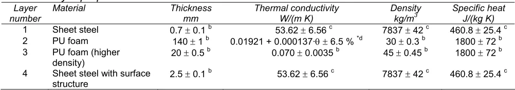
Table 4 Layer properties: Floor. Layer
number
Material Thickness mm
Thermal conductivity W/(m K)
Density kg/m3
Specific heat J/(kg K)
1 Sheet steel 0.7 ± 0.1 b 53.62 ± 6.56 c 7837 ± 42 c 460.8 ± 25.4 c
2 PU foam 140 ± 1 b 0.01921 + 0.000137·θ± 6.5 % *d 30 ± 0.3 b 1800 ± 72 b
3 PU foam (higher
density) 20 ± 0.5
b 0.070 ± 0.0035 b 45 ± 0.45 b 1800 ± 72 b
4 Sheet steel with surface
structure 2.5 ± 0.1
[image:13.595.65.567.604.662.2]b 53.62 ± 6.56 c 7837 ± 42 c 460.8 ± 25.4 c
Table 5 Layer properties: External Wall. Layer
number
Material Thickness mm
Thermal conductivity W/(m K)
Density kg/m3
Specific heat J/(kg K)
[image:13.595.65.398.715.782.2]1 Plywood 10 ± 0.5 b 0.136359 + 0.000175·θ ± 2.5 %*d 850 ± 17 b 1605 ± 7.1 b 2 EPS foam 130 ± 1 b 0.03356 + 0.000127·θ± 4.3 %*d 28 ± 0.28 b 1460 ± 58.4 b 3 Plywood 10 ± 0.5 b 0.136359 + 0.000175·θ ± 2.5 %*d 850 ± 17 b 1605 ± 7.1 b
Table 6 Optical properties of cell surfaces. Solar reflectance
-
Visible reflectance
-
Emissivity
-
Area A
m2
Heat transfer coefficient
Λ20°C
W/(m2 K)
Thermal conductance H20°C
W/K
Ceiling, north (incl. door), east and
west wall 41.745 0.155 6.478
Floor 13.184 0.147 1.941
Thermal bridges guarded zone - - 4.526 ± 10 % b
[image:14.595.69.549.96.187.2]Total 12.945
Table 8 Heat transfer coefficients and thermal conductances of cell to the outside (cell air to outer surface of cell envelope).
Area A
m2
Heat transfer coefficient
Λ20°C
W/(m2K)
Thermal conductance H20°C
W/K
External wall 6.726 0.258 1.736
Thermal bridges outside - - 0.040 ± 10 % b
[image:14.595.63.551.246.311.2]Total 1.776
Table 9 Sensitivity of thermal conductance to changes of important input parameters.
Input parameter Change of input parameter Impact on thermal conductances
HGZ HEW
Thermal conductivity of PU foam ± 5 % ± 3.4 % -
Thermal conductivity of EPS foam ± 5 % - ± 4.7 %
Thermal conductivity of steel ± 10 % ± 0.3 % -
Thermal conductivity of stainless steel ± 10 % ± 0.9 % -
Table 10 Weather data parameters and equipment.
Parameter Unit Type of sensor / measurement Number of
sensors Accuracy
Solar global irradiance, façade plane
W/m2 Pyranometer (Kipp & Zonen CM 21) 1 ± 2 %
Solar global horizontal irradiance
W/m2 Pyranometer (Kipp & Zonen CM 21) 1 ± 2 %
Solar diffuse horizontal irradiance
W/m2 Pyranometer, mounted under the
shading ball of a tracker (Kipp & Zonen CM 11)
1 ± 3 %
Direct-normal irradiance W/m2 Pyrheliometer, mounted in an automatic sun-following tracker (Kipp & Zonen CH 1)
1 ± 2 %
Infrared irradiance, façade plane
W/m2 Pyrgeometers (Kipp & Zonen CG 4) 1 ± 2 %
Outside air temperature, in
front of façade °C Radiation shielded, mechanically ventilated thermocouples 2 ± 0.5 K
Wind speed, in front of façade m/s Ultrasonic anemometer (WindMaster ) 1 ± 1.5 %
Horizontal illuminance Lx Luxmeter (Kipp & Zonen LuxLite, Minolta T-10W)
2 ± 3 %
Pressure hPa Barometric Pressure Measuring Device
(Vaisala PTA 427)
1 ± 0.5 hPa
Relative humidity % Humidity Transmitter (Vaisala HMP
130Y Series)
1 ± 1% (0-90%)
[image:14.595.64.555.358.427.2] [image:14.595.73.553.459.706.2]Parameter Unit Type of sensor / measurement Number of sensors
Accuracy
Air temperatures, inside test cell °C Thermocouple, radiation shielded by two cylinders
8 ± 0.3 K
Air temperatures, in external chamber °C Thermocouple, radiation shielded by two cylinders
5 ± 0.3 K
Air temperatures, in guarded zone, 0.1 m in front of cell surface
°C Thermocouple, radiation shielded by two cylinders
25 ± 0.3 K
Surface temperatures, inner surface of cell envelope
°C Thermocouple 30 ± 0.3 K
Surface temperatures, outer surface of cell envelope
°C Thermocouple 30 ± 0.3 K
Heating power, inside test cell W Electric power (Infratek 106A) 1 ± 0.1 %
Cooling power, inside test cell W Electromagnetic flowmeter
(Endress+Hauser Promag 53H) and temperature difference
measurement (PT100)
3 ± 2 %
Illuminance, horizontal inside cell Lx Luxmeter (Minolta T-1H) 3 ± 2 %
Table 12 Steady-state experiment: Time-averaged values and uncertainties for thermal conductance calculations.
Pel TTC TGZ TEC
Phase A 282.26 W ± 4 W 43.13°C ± 0.5°C 23.50°C ± 0.5°C 23.24°C ± 0.5°C
[image:15.595.65.557.95.287.2]Phase B 145.04 W ± 3 W 36.45°C ± 0.5°C 23.33°C ± 0.5°C 43.74°C ± 0.5°C
Table 13 A summary of the descriptive and comparative statistics.
Parameter Experiment Helios EnergyPlus DOE-2.1e ESP-r
x 33.55 °C 33.44 °C 33.41 °C 33.48 °C 33.18 °C
s 4.89 K 5.05 K 4.94 K 5.00 K 4.97 K
xmax 42.3 °C 42.54 °C 42.33 °C 42.6 °C 42.19 °C
xmin 28.65 °C 28.48 °C 28.57 °C 28.5 °C 28.37 °C
D - 0.11 K 0.14 K 0.06 K 0.36 K
D - 0.31 K 0.18 K 0.25 K 0.37 K
Dmax - 0.8 K 0.72 K 1.22 K 0.94 K
Dmin - 0.01 K 0.00 K 0.00 K 0.01 K
Drms - 0.34 K 0.24 K 0.33 K 0.42 K
D95% - 0.62 K 0.50 K 0.73 K 0.72 K
OU 0.26 K - - - 1.17 K
UR - 0.24 0.14 0.2 0.29
URmax - 0.8 0.6 1.16 0.65
[image:15.595.76.520.405.614.2]Fig. 1 Outdoor view (left) of test cells with two removable façade elements (3.4 m × 3.4 m) and indoor view (right) showing HVAC cabinet and extract and supply ducts.
PCell
PWater Circuit
PEl
PSurround Panel
PSolar PGlazing
Supply Air Extract Air
Guarded Zone External
[image:16.595.78.443.292.439.2]Chamber (Option)
Fig. 2 Concept of test facility with air conditioning of the cell, guarded zone, energy flows into and out of the test cell and optional external chamber.
[image:16.595.71.308.510.685.2]
Fig. 4 Computed heat fluxes at the outer surfaces of the test cell at a temperature difference of 1 K between cell air and guarded zone.
Fig. 5 Computed heat fluxes in a horizontal cross-section of the door.
[image:17.595.70.191.552.733.2]Fig. 7 Location of temperature sensors on inner (30 sensors) and outer (30 sensors) surface of cell envelope. For air temperature (8 sensors) projections on floor, north and west wall are shown.
10 15 20 25 30 35 40 45
100 120 140 160 180
660 680 700 720 740
Cell Air Outside Air North Wall East Wall
West Wall Floor Ceiling South Wall
Te
m
per
at
ur
e (
°C
)
Po
we
r (
W
)
Time (h) Power
Temperatures:
Fig. 8 Mean air temperature inside cell and outside, mean surface temperatures of all six faces and heating power inside the cell as a function of time during phase B of the steady-state experiment (duration 96 h).
North Ceiling
Floor
West East
[image:18.595.79.289.332.569.2]8 10 12 14
1 2 3 4
15 20 25 30 35 40
Temperature (°C) External Wall 1
2
14
T
he
rm
al C
on
du
cta
nc
e (
W
[image:19.595.76.265.73.254.2]/K
Fig. 9 Comparison of thermal conductances HGZ and HEW as function of temperature found
by simulation and the steady-state experiment.
20 25 30 35 40 45
0 100 200 300 400
0 100 200 300 400 500 600
Te
m
pe
rat
ur
e (
°C
)
Pow
er
(
W
)
Time (h)
Power Cell air
[image:19.595.78.288.291.469.2]Surfaces
Fig. 10 Measured pseudo-random internal heating power, cell air temperatures (total eight sensors) and mean surface temperatures of all six outer cell surfaces.
25 30 35 40 45
0 100 200 300 400 500 600
Experiment DOE-2.1E EnergyPlus ESP-r Helios
Te
m
pe
ra
tu
re (
°C
)
Time (h)
0 0.5 1 1.5 2 2.5
0 100 200 300 400 500 600
Total
O
ut
pu
t Un
ce
rt
ai
nt
y
(K
)
Time (h) OU
[image:20.595.79.256.81.300.2]Experiment + OUESP-r