Int. J. Electrochem. Sci., 14 (2019) 1529 – 1545, doi: 10.20964/2019.02.47
International Journal of
ELECTROCHEMICAL
SCIENCE
www.electrochemsci.org
Numerical Study of Stainless Steel Pitting Process Based on the
Lattice Boltzmann Method
Jing Cui, Fan Yang, Ting- Hao Yang, Guang-Feng Yang*
Civil Aviation University of China Airport College, Tianjin 300300,China
*E-mail: [email protected] & [email protected]
Received: 12 September 2018 / Accepted: 27 Nobember 2018 / Published: 5 January 2019
The application of computers to numerical calculations has become an important means of studying corrosion problems, and in this work, the lattice Boltzmann method (LBM) was used to numerically simulate the pitting corrosion of stainless steel. The multi-phase multi-component model, electrochemical reaction model and phase change model were applied to construct a new lattice Boltzmann corrosion model based on the Lattice Boltzmann method and corrosion kinetics behaviour. Moreover, the passivation probability was employed for modifying the chemical reaction rate, and the Volume of Pixel method was adopted for treating the migration of the solid boundary. A realistic liquid corrosion environment was constructed using the lattice Boltzmann method to simulate the concentration profiles of different components. The pitting corrosion characteristics of stainless steel were investigated numerically using this proposed model. Moreover, the unsteady topological structures of the corrosion pit and the instantaneous concentration distribution of the various components were obtained. In addition, specific chemical reactions and electrochemical reactions were introduced into the corrosion model to ensure the conservation of mass. The reaction mechanism of stainless steel pitting corrosion was clearly explained by using this model.
Keywords: Lattice Boltzmann method, Pitting on stainless steel, Electrochemical reactions, Volume of Pixel, Passivation probability
1. INTRODUCTION
equipment, affecting the normal operation of the equipment. Thus, pitting increases the maintenance cost of the equipment. Therefore, prediction of pitting and protection of metal from pitting are highly important for saving metal resources and prolonging the service life of metal equipment.
The pitting corrosion of stainless steel can be divided into two stages, namely, the initiation stage and the development stage. Currently, three widely accepted pitting models have been used for theoretical understanding of pitting corrosion. The first is the penetration theory[1] proposed by Zamaletdinov[2] that states that metal ions accelerate the rate of transport from the substrate to the boundary of the passive film/solution, resulting in the initiation of pitting on the interface of the passive film and metal substrate. When the pitting grows to a certain size, the passive film will break down, and the pitting would nucleate. Second, adsorption theory developed by Marcus[3] argues that competitive absorption may occur on the surface of the passive film by the chloride ions and hydroxyl groups, thereby forming metal chloride with strong solubility that will cause the passive film to grow at a rate lower than the dissolution rate. The weak part of the passive film is the first to rupture and exposes the substrate, while the chloride ions will also be adsorbed on the metal substrate surface, continuing to replace the hydroxyl groups and preventing the formation of the passive film, leading to nucleation of pitting. Third, the local failure theory of passive film[4] proposed by Xu[5] suggests that the passive film could be ruptured under mechanical stress. When the film is thinned to a certain extent, the film will also rupture under the action of electron contraction pressure, and then the active dissolution occurs at the crack, and the local acidification behaviour may be accompanied by the film thinning that facilitates the development of pitting nucleation. Likewise, many theories have been proposed to describe the development stage of pitting. Currently, the autocatalytic corrosion model of obliterated pitting corrosion occurring in the pit[6] has been generally accepted (Zhang[7] proposed that once the steady pitting is formed, the metal in the pit is activated and dissolved and acts as the anode, while the passive film outside the pit acts as the cathode. Therefore, the "small anode and large cathode" activation-passivation battery is formed around the pit.).
Currently, the finite element method, molecular dynamics simulations and cellular automata method are widely used to simulate corrosion phenomenon. For example, Vagbharathi[12] constructed a steady pitting model using the finite element method. Xu[13] used molecular dynamics model to study the adsorption of 2-pyridine formaldehyde thiosemicarbazone and 4-pyridine formaldehyde thiosemicarbazone (two chemical reagents) on iron ions in a sulphuric acid solution in order to evaluate the corrosion inhibition performance of the two abovementioned chemical reagents. Wang[14] simulated the metastable pitting process of stainless steel using cellular automata. However, each of these methods has its drawbacks. The finite element corrosion model used to simulate the corrosion process strongly depends on method used to treat the thinning of the local material, which is arbitrary and inadequate in the simulation and faces difficulties in addressing the complex boundary and the multi-phase (solid-liquid gas three-phase) problem. Molecular dynamics simulations are mainly applied to study the influence of different particles on the corrosion of materials, but their computational cost is too high due to the high accuracy of the simulations. Generally, cellular automaton is used to describe the morphology of pitting, mostly focusing on qualitative change analysis. The mass transport of different components and corrosion chemical reaction are modelled using oversimplified assumption during the calculations, making the simulations insufficiently accurate.
In recent years, the lattice Boltzmann method (LBM) that has been less frequently used to simulate corrosion has been developed rapidly worldwide. The LBM method has been applied successfully in the dynamic system with microscopic interactions, for example, for multicomponent systems, interfacial kinetics and chemical reactions. LBM method not only guarantees the rationality of the model or method but also takes into account the actual computational cost, enabling its use for the simulation of the corrosion process. Wells[15] and Janecky[16] used the lattice Gas Automata (LGA) model to model the surface reaction. In their model, the phase change problem and the chemical reaction between the solution and the solid interface are not considered. In 2000, He[17] first combined a chemical reaction with the LB method, providing a clear approach for dealing with the coupling of the fluid-wall surface reaction and diffusion for simulating corrosion. In 2002, Kang[18] studied the flow and transportation of single-phase fluid in the dissolution-precipitation problem. Kang believed that the LB method should be combined with the VOP (Volume of Pixel) method to simulate the transport of the components during the corrosion process. Subsequently, Kang[19] extended his model to address the mass transport problem in multiphase multicomponent systems. To solve the problem of phase transition and solution precipitation in multiphase flow, Chen[20] combined the LB method with the VOP method at the pore scale, successfully solving the problems of phase separation, mass transport, chemical reaction and solution precipitation in multiphase flow. Nogues[21] and Yoon[22] studied the corrosion of carbonate using the pore network model. Liu[23] used the D3Q19 model to simulate the corrosion of
rock. Huber[24] studied the dissolution process of minerals using LBM combined with the phase field method. All of the above studies provide theoretical support for the simulation of corrosion conditions with LBM. However, the existing Lattice Boltzmann corrosion models cannot simulate the corrosion of specific metal materials, and use more chemical corrosion methods, only considering anode solid corrosion and rarely treating the cathodic reactions.
remedy the deficiency of the existing LBM corrosion model. The passivation probability was added to the LBM corrosion model to modify the chemical reaction rate and the morphology of the corrosion pits. The entire process of pitting corrosion on stainless steel surface was simulated using the improved model, facilitating the elucidation of the morphologies of the pitting pits and the variation in the concentration of each component.
2. LB MODEL FOR PITTING
The LB model for pitting consists of the following five sub-models:
(1) Electrochemical reaction model solving several problems related to the electrochemical reaction, dissolution of the anode metal and precipitation of the cathode corrosion products.
(2) Multicomponent model for dealing with multiphase flow. (3) Model for multicomponent mass transport.
(4) Solid boundary reaction kinetics model for phase transformation. (5) Passivation model for modifying the corrosion rate.
2.1 Electrochemical reaction model
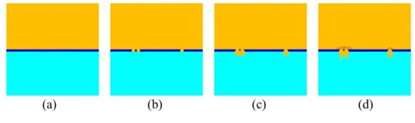
The objective of the present work is to simulate the pitting process of stainless steel in an oxygen-containing NaCl solution. The pitting process is described in Figure 1.
Figure 1. Schematic illustration of pitting model
[image:4.596.147.444.496.584.2]
will be sustained (This process cannot be described by specific chemical reaction equations because the passivation film is very thin and has an extraordinarily complex composition). Then, metastable pitting will begin (Some researchers believe that metastable pitting has a hemispherical morphology[25]). Most metastable pitting will repassivate and stop growing, while only a fraction will develop into stable pitting. During steady pitting process, the degree of corrosion will increase (shown in Figure 1(c)) and secondary holes may appear at the bottom of the corrosion pit (shown in Figure 1(d)). The chemical reactions in the steady pitting process of pitting are given by:
Anode: Fe2eFe2 (1)
Cathode: 2H O2 O2 4e 4OH
(2) Precipitation reaction: 2
2
e 2 ( )
F OHFe OH (3) Precipitation-oxidation reaction: 4Fe OH( )22H O2 O24 e(F OH)3 (4) Ferrous oxidation: 2 3
e
F e Fe (5) Iron ion hydrolysis: 3
2 3
e 3 ( ) 6
F H OFe OH H (6) Autocatalytic reaction: 2
2
e 2
F HFeH (7) Neutralization reaction: H OH H O2
(8)
The metal in the pit undergoing active dissolution acts as the anode, and the region of the passivation film outside the pit acts as the cathode. Thus, “the small anode” reacting according to (1) and the “large cathode” reacting according to (2) comprise the whole corrosive battery system. The concentration of the hydroxyl ions around the opening of pit will increase gradually as a result of reaction (2) with the metal ions in the pit diffusing out. Metal ions react with hydroxyl ions according to (3) and (4) to give rise to the precipitation of hydroxide around the pitting port. As the metal in the pit continues to corrode and dissolve, the amount of the metal ions gradually increases, and then metal ions will hydrolyse (Reaction (6)). The increase in the number of the hydrogen ions in the pit creates an acidic environment that accelerates corrosion (Reaction (7)), as shown in Figure 1(d), with neutralisation reactions also occurring at any time inside or outside the pit (Reaction (8)).
2.2 Multicomponent LB model
The motion of a fluid is described by a set of particle distribution functions. Based on the simple and popular BGK collision operator, the evolution equation of the distribution functions is given by
1
, , , ,
x e x x eq x
v
f c t t t f t f t f t
(8)
where f
x,t is the density distribution function of the corrosion solution at the lattice site x and time step t, and v is the dimensionless relative time. The equilibrium distribution function feq for the D2Q9[27-31] lattice has the form. 2 2
2 4 2
3 9 3
1 ·
2 2
· eq
f
c c c
e u e u u (9)
The weight factors are given by 0=4 / 9,1 4 =1 / 9 and 5 8 =1/ 36. The solution density
and velocity u are obtained from the first and second moments of the density distribution functions:
f
f u e
(11)
In Shan and Chen’s pseudopotential model[32-34], to reduce the error and ensure the stability of the calculation results, molecular force is used to modify u. The molecular force is written as
2 1 N G w
F x e x e e (12) where G is the interaction strength, and
2
w
e
are the weights. If only four nearest neighbours e1 4 2=1 and four next-nearest neighbours2
5 8 =2
e are considered, w
1 1/ 3 and
2 1/12w . Forces between the solution and solid phase are also present and are given by
2 1
N
w ww w s
F x e x e e (13)
where w[26-30] determines the strength of the interaction between the solution and the solid wall. s represents the wall density[31-33], and is 1 for solid nodes and 0 for solution nodes.
The modified velocity is expressed as
v
F
u u
(14)
where F is the sum of the forces and u’ is obtained using Eq. (11).
2.3 LB for mass transport
Several studies have sought to solve the convection diffusion equation of solute transport using the LBM. The following evolution of the LB equation is used to describe species transport:
, , , ,
,
1
, , , ,
x e x x eq x
k k k k
k g
g c t t t g t g t g t (15)
where gk, is the concentration distribution function for component k, and
k g, is the dimensionless relative time for the concentration distribution[34-36]. An equilibrium distribution that is linear in u is adopted:, ,
1 · 2 eq
k k k
g C J
e u
(16) where C is the concentration and Ji is given by
,0 ,
,0
0
(1 ) / 4 1, 2,3, 4
k k k J J J
(17)
where the rest fraction J0 can be selected in the range from 0 to 1. The concentration is given by ,
k k
C g
(18) The diffusivity D is related to the relaxation time by
,0
,
1
1 0.5
2
k k k g
D J
(19)
2.4 Solid boundary reaction kinetic model
According to Reaction (1), the volume[23] of iron is reduced by
1 2
s
s aq
Fe
Fe O
dV
AV k C
dt (20)
The passivation film is complex and very thin, so that the damage process of the passivation film is modelled by simulating metal corrosion. The volume of the passivation film node is reduced by
s
s aq
PF
PF PF Cl
dV
AV k C
dt (21)
According to the Reaction (2), the volume of the corrosion product is increased according to
3 3 3 e( )
e( ) 2
s
s aq
F OH
F OH Fe
dV
AV k C
dt (22) where
e
F
V ,VF OHe( )3and VPF s are the dimensionless volumes of iron, iron oxide-hydroxide and passivation film, respectively. VFe ,
3
e( )
F OH
V and
s
PF
V are the molar volumes of iron, iron oxide-hydroxide and passivation film, respectively. k is the reaction rate constant. The concentration of the components is calculated using (26), (27) and (28). The dimensionless volumes of the three solid components are updated at each time step explicitly according to the following equations:
2
e Fe 1 O
F Fe
V t t V t AV k C t
(23)
PF PF PF PF Cl
V t t V t AV k C t
(24)
3
3
3 ( ) ( 3
H) )
e(O Fe OH Fe OH 2 Fe
F
V t t V t AV k C t (25)
If the values of VFeand
s
PF
V reach zero, corrosion is complete, and the solid node is removed and converted to a fluid node. Meanwhile, the fluid flow and mass information in this new fluid node must be initialised. By contrast, when the volume of the iron oxide-hydroxide node exceeds a certain threshold value, precipitation occurs and one of the fluid nodes with the concentration that reached saturation becomes a solid node.
The boundary concentrations[37] at the solution-solid interface for the aqueous phase are given by Eqs. (26), (27) and (28):
2
2 2
( )
(a ) 1 ( )
O aq
O q O aq
C
D k C
n
(26)
l ( )
l (a ) l ( )
C aq PF
C q C aq
C
D k C
n
(27)
3 3 3 2 e aq aq aq Fe F Fe C
D k C
n
(28)
where k is the reaction rate constant and CO2(aq), CCl- and CFe3+(aq) are the reaction-boundary concentrations of oxygen, chloride ion and iron ion, respectively. The tern n represents the surface normal that points into the solution. DO2(aq), DCl-(aq) and DFe3+(aq) are the diffusivities of oxygen chloride ions and iron ions, respectively.
2.5 Passivation model
probability, defined as the Passivation Probability, will cause the corrosion rate to slow down and the shape of the pitting to be asymmetric. The Passivation function is written as
0 ( )
=
1 ( )
R P R P
(29)
where
is the passivation probability coefficient, and R is a random real number between 0 and 1. P is the passivation probability. Therefore, Eq. (23) must be revised to
1 2e Fe O
F Fe
V t t V t AV k C t (30)
the probability-VOP coupling makes the morphology of pitting random and the corrosion rate asymmetric.
3. SIMULATION RESULTS AND DISCUSSION
[image:8.596.69.537.498.637.2]Based on the Lattice Boltzmann corrosion model, the pitting process of stainless steel was simulated. A 160 × 160 lattice with the thickness of passivation film of 5 layers was used. In the calculation of the interface between the passivation film and the corrosion solution, three points were selected as the initiation points of the pitting corrosion. The coordinates of the three points were (45,80), (55,80), (120,80). The purpose of the selection of various distances between the initiation points is to simulate the corrosion pits merging gradually in the corrosion process when the adjacent pits are close to each other. The boundary around the liquid was treated by non-equilibrium extrapolation, while the solid interface was treated by a rebound boundary. All of the parameters are dimensionless and are obtained from the transformation rules[20,28,34] in Table 1.
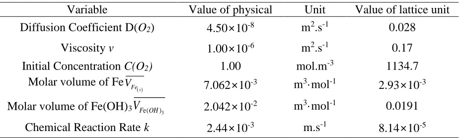
Table 1. Parameters used in the simulation
Variable Value of physical Unit Value of lattice unit Diffusion Coefficient D(O2) 4.50×10⁻⁸ m2.s-1 0.028
Viscosity v 1.00×10⁻⁶ m2.s-1 0.17
Initial Concentration C(O2) 1.00 mol.m-3 1134.7
Molar volume of Fe s
Fe
V 7.062×10⁻³ m3·mol-1
2.93×10⁻³ Molar volume of Fe(OH)3VF OHe( )3 2.042×10⁻² m
3·mol-1 0.0191
Chemical Reaction Rate k 2.44×10⁻³ m.s-1 8.14×10⁻⁵
The pitting morphology of stainless steel at different times and the concentration distribution of each component in the corrosion environment were obtained by the numerical simulations.
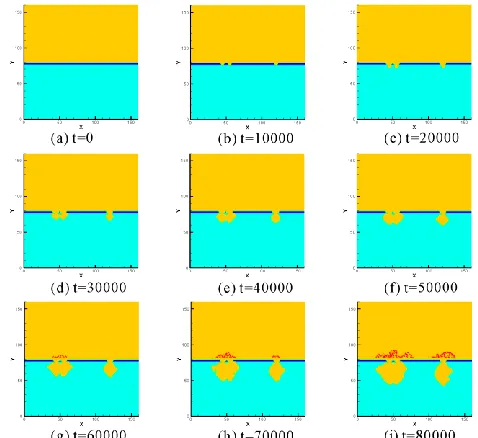
(this is consistent with the first of the pitting growth patterns mentioned in reference[9]) in Fig. 2(f), confirming that the larger pits are apparently composed of several smaller pits, and some pits are formed below the previously formed pits as proposed by Jing[39]. During the process of the pitting transition from the metastable to steady state, iron oxide-hydroxide was formed at the pits’ opening and gradually covered the pits opening, as shown in Fig. 2(g). Meanwhile, experiments conducted by Ernst[40] showed that the pit opening is covered by corrosion products, and Hu[41] used SEM to observe the corrosion products covered around the pitting opening. Except for the primary pit developed by initial pitting nucleation, on the entire pitting process, the secondary pit at the bottom of the primary pit (which was consistent with the second pitting growth mode mentioned in reference[9]) would also grow to maintain the development of the pitting at greater metal depth. Frankel[42] measured the current density and found a secondary pit at the bottom or at the edge of the primary pit.
[image:9.596.172.411.264.483.2]Figure 2. Morphology evolution of the corrosion pit
Figure 3. Morphology evolution of the passive film
[image:9.596.146.448.516.652.2]
The calculation results were consistent with theory proposed by Marcus[48] that the passivation film is gradually thinned, causing the base metal to contact the corrosion solution. Thereafter, the anode was in contact with the corrosion solution as shown in Figure 3(f). When the anodic metal began to dissolve, cathodic action occurred simultaneously on the surface of the passivation film, resulting in a large amount of hydroxyl ions produced by the cathode and leading to the decrease in the damage rate of the passivation film. The simulation results in Figure 3(f) are in agreement with the experimental findings[48] that the hydroxide produced by the cathode adsorbs on the metal surface, giving rise to the repassivation of the metal and the reduction in the thinning rate of the passivation film.
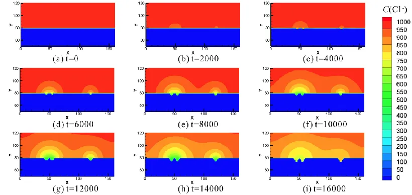
[image:10.596.84.494.382.576.2]The distribution of chloride ion concentration during the damage stage of the passive film is shown in Figures 4(a)-(f). At first, chloride ion was uniformly distributed in the solution, and at the site of pitting initiation, chloride ion and passivated film reacted with each other, resulting in the decrease in the chloride ion concentration near the pitting initiation site. The simulation results in Figure 4(f) were consistent with the Pardo’s theory that the passivating film is eroded by chloride ions, resulting in initial pitting[49]. Meanwhile, Zhang[50] also obtained conclusions that were consistent with the simulation results shown in Figure 4 by using SIMS. Under the action of the concentration difference, chloride ions migrated to the vicinity of pitting initiation. As the passivation film became thinner, the consumption of chloride ion increased[39,48,51,52,53,54].
Figure 4. Time evolution of the chloride ion concentration profile
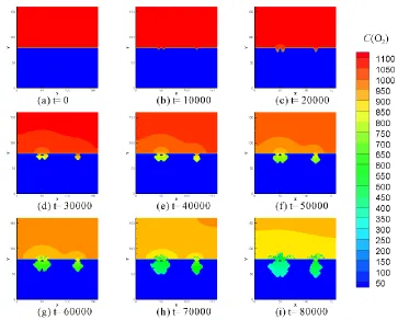
pitting also found that the cathode reaction is carried out on the surface of the stainless steel passivating film, giving rise to oxygen consumption. With the variation of time, the volume of the dissolved anodic metal gradually increased, and oxygen permeated into the corrosion pit[56]. For t=40000, the two pits close to each other merged, and the oxygen concentrated in the pits close to each other began to flow through the corrosion interface after the corrosion pits fused (the oxygen outside the pits diffused into the hole, and the difference in oxygen concentration between the inside and outside of the hole accelerated the dissolution of the metal[57]). As shown in Fig. 5(g), when the pits opening was precipitated by corrosion products, the precipitation hindered the diffusion of the corrosion solution into the pits, resulting in the gradual decrease of the oxygen concentration of the corrosion solution in the pits, confirming the conclusion[58] that the deposition (corrosion products) outside the pit hindered the transport of dissolved oxygen, resulting in a high oxygen concentration outside the pit and a low oxygen concentration inside the pit.
Figure 5. Time evolution of the corrosion solution (oxygen) concentration profile
[image:11.596.116.479.294.586.2]
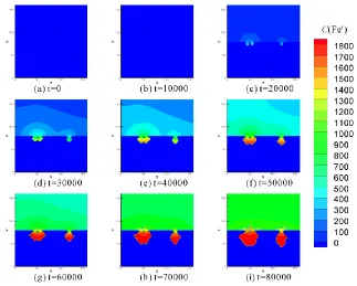
two corrosion pits close to each other merged. Iron ions diffused to the opening of the pits and reacted with the hydroxyl ions outside the pits to produce iron oxide-hydroxide. Once the concentration of iron oxide-hydroxide reached its saturation concentration, a precipitation reaction occurred (A previous study[60] of the corrosion products suggested that when the corrosion product concentration reached its supersaturated concentration, the corrosion product would precipitate. Chen also introduced the concept of saturated concentration in his studies[20,32] on the precipitation of porous media.). The formation of pits' opening precipitation hindered the diffusion of iron ions out of the pits and the increase in the iron ion concentration in the pores shown in Fig. 6(i) accelerated the hydrolysis of iron ions, corresponding to the experimental finding that the metal ions in the pits hydrolyse to produce large amounts of hydrogen ions[61]. The simulated morphology of the pit had a tapered appearance that was similar to the experimentally obtained pit shape[62].
Figure 6. Time evolution of the corrosion products (iron ions) concentration profile
[image:12.596.136.459.277.536.2]
Suter[29] measured the pH in the pits and found that there were many hydrogen ions in the pits, giving rise to an acidic environment inside the pits. Under the strong acidic environment inside pits, the metal node at the corrosion interface underwent reaction (7), leading to the accumulation of iron ions in the pore, and the promotion of the hydrolysis reaction (6) that increased the dissolution rate of the metal and generated the autocatalytic effect[63-68]. This finding is in good agreement with the results of Jing[39], who insisted that local acidification within the pits will accelerate the rate of metal dissolution. Thus, the pitting process entered the steady state[69].
[image:13.596.141.457.222.410.2]Figure 7. Time evolution of the hydrogen ion concentration profile
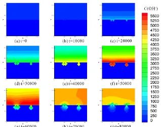
Figure 8. Time evolution of hydroxyl ion concentration profile
[image:13.596.136.454.449.699.2]
with time is shown in Figures 8(a)-(i). Prior to pitting, the hydroxyl ions were distributed uniformly. When pitting nucleated, because of the high potential of the passivation film outside the pit, corrosion due to oxygen atmosphere reacting at the cathode occurred as described by reaction (2); this produced hydroxyl ions that then diffused to the region with the relatively low hydroxyl ion concentration. It was observed that the concentration of hydroxyl ions reached the peak at t=50000. Hydroxyl and iron ions diffused and were consumed prior to t=60000, and when the two iron came into contact with each other, iron oxide-hydroxide was produced[56]. The highest hydroxyl ion and iron ion concentrations were obtained near the opening of the pit. Several previous studies[56,60] also found that the passivating film outside the pits acted as the cathode that consumed dissolved oxygen and produced OH-. The concentration of iron oxide-hydroxide first reached its saturation concentration in the region near the opening of the pit, and then the precipitation reaction occurred, hindering the ion transport inside and outside the pit. This finding is in good agreement with the experimental result of Tian[55], who suggested that iron hydroxide is a corrosion product that covers the pitting. Therefore, the hydroxyl ions in the pit were neutralised by the hydrogen ions in the pit, as shown in Figures 8(g)-(i), causing the concentration of the hydroxide ions in pits to be significantly lower than that outside of the pits[60].
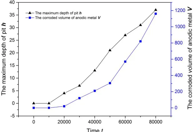
[image:14.596.162.470.463.674.2]Both the anodic metal volume corroded by the electrolyte and the maximum depth[70] of the pits were accurately calculated from the simulation results. After the pitting simulation was completed, the relationship between the anodic metal volume corroded by the electrolyte and time was obtained as shown in Figure 9, with the variation of the maximum depth of the pits with time also shown in Figure 9. An examination of Figure 9 that the anode metal was not corroded until t=10000. With longer time, the passivation film at the site of pitting initiation was completely destroyed, and the anode metal was corroded at t=20000.
Figure 9. Variation of the degree of corrosion with time
this finding is observed because the pitting opening appears to be blocked by corrosion products for t=60000, and the acid environment in the pits leads to the self-catalytic reaction such that the corrosion rate will increase at this time. Both the simulation results presented in Figure 9 and the experimental results obtained by Du[59] found a turning point for the corrosion rate during the pitting process, and the amount of the corroded metal increased with time.
While the Cellular Automaton method has been more widely used to simulate pitting corrosion, the LBM method used in this work represents a breakthrough innovation for simulation of metal pitting. Wang[14] simulated the metastable pitting process of stainless steel using the cellular automata method and obtained the corrosion morphology of single-pit pitting and double-pit pitting. However, both the pitting corrosion morphology of the pit and the variation of the different components in the liquid environment around the pit were also obtained using the LBM corrosion model in this paper. Malki'[71] used the CA corrosion model to simulate the growth process of pitting, and "Pseudo electro-migration" was assumed to be the mechanism of the electrolyte transport, which does not correspond to the Navier-Stokes equations. By contrast, the multicomponent LB model used in this works corresponds to the Navier-Stokes equation and can be used to describe the flow diffusion of liquid components, enabling more realistic simulation of the liquid environment using the LBM method. Additionally, Li[72] also used cellular automata to simulate the metastable pitting process. He used the LGA model to simulate liquid diffusion in the corrosion model, which was more consistent with true liquid diffusion than the pseudo electro-migration. Nevertheless, the LGA method also had some disadvantage such as the statistical noise arising from the Boolean variables and the violation of the Galilean invariance. Therefore, the use of the LBM method for pitting simulation not only overcame the disadvantages of cellular automata but is also innovative.
4. CONCLUSION
In this paper, a pitting model was constructed by combining the lattice Boltzmann method and the volume of pixel method in order to simulate the entire process of stainless steel pitting corrosion. The specific chemical reactions and electrochemical reactions were added into the corrosion model that clearly described the reaction mechanism of stainless steel pitting corrosion. The following conclusions were obtained from the simulations:
1) In the entire corrosion process, the flow field and concentration fields of different components in the solution were described by LBM, enabling simulations of the realistic liquid corrosion environment. Second, the passivation probability was employed for modifying the pit topography, giving rise to the asymmetric morphology of the corrosion pit. The VOP method combined with LBM not only simulated the control of the corrosion reaction rate but also easily handled the transformation between the solid and liquid phases in the corrosion process, rather than relying on random conversion rules. Finally, electrochemical corrosion was simulated through the cathode interacting with the anode.
steady-state. In the steady state process, the acidic environment in the pitting hole provides the conditions for the autocatalytic effect of the anode metal, thereby accelerating the corrosion reaction, causing the pitting to extend deep into the metal and leading to the generation of secondary pores.
ACKNOWLEDGEMENT
This work was supported by National Natural Science Foundation of China(U1633111,51206179) and the Fundamental Research Funds for the Central Universities(3122017036, 3122017040) and the work supported by Fundamental Research Funds for the Central Universities(ZYGX2018044).
References
1. O. Tatsuhiro, Corros. Sci., 31(1990) 453. 2. I. I. Zamaletdinov, Prot. Met., 43 (2007) 470.
3. P. Marcus, V. Maurice, H. Strehblow, Corros. Sci., 50 (2008) 2698.
4. Y. Xu, M. Wang and H.W. Pickering, J. Electrochem. Soc., 140 (1993) 658. 5. A. Pardo, M.C. Merino and A.E. Coy, Corros. Sci., 50 (2008) 1796.
6. S.H. Xiong, Z.P. Zhu and L.L. Jing, Anti-Corros. Methods Mater, 59 (2012) 3. 7. Z.Y. Zhang, Z.Y. Wang and Y.M. Jiang, Corros. Sci., 62 (2012) 42.
8. P. Ernst and R.C. Newman, Corros. Sci., 44 (2002) 943.
9. C.Y. Wang, M.E. Wang and J. Zhu, Journal of Nanjing Tech University, 21 (1999) 26. 10. R. Smallwood, R.B. Pearson and A.P. Brook, Wear, 125 (1988) 97.
11. H. Jung, K. Kwon–J and E. Lee, Corros. Eng., Sci. Technol., 46 (2011) 195. 12. A.S. Vagbharathi and S. Gopalakrishnan, Adv. Mater. Res., (2014) 2979.
13. B. Xu, W.Z. Yang, Y. Liu, X.S. Yin, W.N. Gong and Y.Z. Chen, Corros. Sci., (2014) 78. 14. H.T. Wang and E.H. Han, Materials & Corrosion, 66 (2015) 925.
15. J.T. Wells, D.R. Janecky and B.J. Travis, Phys. D (Amsterdam, Neth.), 47 (1991) 115. 16. W.E. Seyfried, D.R. Janecky and M.J. Mottl, Geochim. Cosmochim. Acta, 48 (1984) 557. 17. X. Y. He, N. Li and B. Goldstein, Mol. Simul., 25 (2000) 145.
18. Q. Kang, D. Zhang and S. Chen, Phys. Rev. E: Stat., Nonlinear, Soft Matter Phys., 25 (2002) 145. 19. Q. Kang, P.C. Lichtner and H.S. Viswanathan, Transp. Porous Media, 82 (2010) 197.
20. L. Chen, Q. Kang, B.A. Robinson,Y. He and W. Tao, Physical Review E Statistical Nonlinear & Soft Matter Physics, 87 (2013) 043306-1.
21. J.P. Nogues, J.P. Fitts and M.A. Celia, Water Resour. Res., 49 (2013) 6006 22. H. Yoon, A.J. Valocchi and C.J. Werth, Water Resour. Res., 48 (2012) 2478. 23. M. Liu and P. Mostaghimi, Chem. Eng. Sci., 161 (2017) 360.
24. C. Huber, B. Shafei and A. Parmigiani, Geochim. Cosmochim. Acta, 124 (2014) 109. 25. B. Maier and G.S. Frankle, J. Electrochem. Soc., 157 (2010) 302.
26. Y.T. Mu, L. Chen and Y.L. He, Build. Sci., 104 (2016) 152.
27. J. Pedersen, E. Jettestuen and M. V. Madland, Adv. Water Resour., 87 (2015) 68. 28. L. Chen, Q. Kang and Y.L. He, Langmuir., 28 (2012) 11745.
29. L. Chen, H.B. Luan and Y.L. He, Int. J. Therm. Sci., 51 (2012) 132. 30. A. Atia and K. Mohammedi, World J. Eng., 12 (2015) 353.
31. L. Chen, Q. Kang and Y. Mu, Int. J. Heat Mass Transfer, 76 (2014) 210.
32. L. Chen, Q. Kang, Q. Tang, B.A. Robinson, Y. He and W. Tao, International Journal of Heat & Mass Transfer, 85 (2015), 935.
37. M. Vincent and P. Marcus, Progress in Corrosion Science and Engineering I, (2009). 38. C.J. Boxley and H.S. White, Journal of the Electrochemical Society , 151 (2004) 265. 39. L. Jing, Z. Zhu and S. Xiong, Anti-Corrosion Methods and Materials, 59 (2012) 3.
40. P. Ernst, N.J. Laycock, M.H. Moayed and R.C. Newman, Corrosion Science, 39 (1997) 1133. 41. L.H. Hu, N. Du, M. Wang and Q. Zhao, Journal of Chinese Society for Corrosion and Protection,
27 (2007) 233
42. G.S. Frankel, National Association of Corrosion, 1986.
43. J. Lv, , W. Guo and T. Liang, Journal of Alloys & Compounds, 686 (2016) 176.
44. J. Shi, W. Sun, J. Jiang and Y. Zhang, Construction & Building Materials, 111 (2016) 805. 45. G. Meng, Y. Li, Y. Shao, T. Zhang, Y. Wang and F. Wang, Journal of Materials Science &
Technology, 30 (2014) 253.
46. Z. Chen and F. Bobaru, Peridynamic modeling of pitting corrosion damage, J.Mech. Phys. Solids,78 (2015) 352.
47. G.S. Frankel, T. Li and J. R. Scully, Journal of the Electrochemical Society, 164 (2017) 180. 48. P. Marcus, V. Maurice and H. Strehblow, Corrosion Science, 50 (2008) 2698.
49. A. Pardo, M.C. Merino, A.E. Coy, R. Arrabal, F. Viejo and E. Matykina, Corrosion Science, 50 (2008) 823.
50. H. Zhang, V. Vignal, O. Heintz and J. Peultier, Revue De Métallurgie,108 (2011) 9. 51. J. Gao,Y. Jiang, B. Deng, Z. Ge and J. Li, Electrochimica Acta, 55 (2010) 4837.
52. C. Gouveia-Caridade, M.I.S. Pereira and C.M.A. Brett, Electrochimica Acta, 49 (2004) 785. 53. Y. Tang, Y. Zuo, J. Wang, X. Zhao, B. Niu and B. Lin, Corrosion Science, 80 (2014) 111. 54. T. Sourisseau, E. Chauveau and B. Baroux, Corrosion Science, 47 (2005) 1097.
55. W. Tian, N. Du, S. Li, S. Chen and Q. Wu, Corrosion Science, 85 (2014) 372.
56. Z. Feng, X. Cheng, C. Dong, L. Xu and X. Li, Journal of Nuclear Materials, 407 (2010) 171. 57. Y. Chao, N. Du, W. Tian, Q. Zhao and L. Zhu, Journal of Chinese Society for Corrosion &
Protection, 35 (2015) 38.
58. W. Tian, S. Li, N. Du, S. Chen and Q.Wu, Corrosion Science, 93 (2015) 242. 59. N. Du, W. Tian, Q. Zhao and S. Chen, Acta Metallurgica Sinica, 48 (2012) 807. 60. G.S. Frankel, Journal of the Electrochemical Society, 145 (1998) 2186.
61. M.P. Ryan, D.E. Williams, R.J. Chater, B.M. Hutton and D.S. McPhail, Nature 415 (2002) 770. 62. A. Broli, H. Holtan and T.B. Andreassen, Materials & Corrosion, 27 (2015) 497.
63. T. Suter, E.G. Webb, H. Bohni and R.C. Alkire, Journal of the Electrochemical Society, 148 (2001) 174.
64. Z. Zhang, C. Cai, F. Cao, Z. Gao, J. Zhang and C. Cao, Acta Metallurgica Sinica(English Letters), 18 (2005) 525.
65. S.R.F. Batista and S.E. Kuri, Anti-Corrosion Methods and Materials, 51 (2004) 205. 66. K.R. Tarantseva, Protection of Metals & Physical Chemistry of Surfaces, 46 (2010) 139. 67. Y. Tsutsumi, A. Nishikata and T. Tsuru, Corrosion Science, 49 (2007) 1394.
68. Z. Zhang, Z. Wang, Y. Jiang, H. Tan, D. Han, Y. Guo and J. Li, Corrosion Science, 62 (2012) 42. 69. P.C. Pistorius and G.T. Burstein, Philosophical Transactions of the Royal Society A Mathematical
Physical & Engineering Sciences, 341 (1992) 531.
70. K.R. Tarantseva, Protection of Metals & Physical Chemistry of Surfaces, 46 (2010) 139. 71. B. Malki and B. Baroux, Corrosion Science, 47 (2005) 171.
72. L. Li, X. Li, C. Dong and Y. Huang, Electrochimica Acta, 54 (2009) 6389.