Angular momentum transport by the GSF instability: non-linear simulations at the equator

simulations at the equator

.

White Rose Research Online URL for this paper:

http://eprints.whiterose.ac.uk/146375/

Version: Published Version

Article:

Barker, AJ orcid.org/0000-0003-4397-7332, Jones, CA and Tobias, SM (2019) Angular

momentum transport by the GSF instability: non-linear simulations at the equator. Monthly

Notices of the Royal Astronomical Society, 487 (2). pp. 1777-1794. ISSN 0035-8711

https://doi.org/10.1093/mnras/stz1386

This article has been accepted for publication in Monthly Notices of the Royal Astronomical

Society. ©: 2019 The Author(s) Published by Oxford University Press on behalf of the

Royal Astronomical Society. All rights reserved.

eprints@whiterose.ac.uk

https://eprints.whiterose.ac.uk/

Reuse

Items deposited in White Rose Research Online are protected by copyright, with all rights reserved unless

indicated otherwise. They may be downloaded and/or printed for private study, or other acts as permitted by

national copyright laws. The publisher or other rights holders may allow further reproduction and re-use of

the full text version. This is indicated by the licence information on the White Rose Research Online record

for the item.

Takedown

If you consider content in White Rose Research Online to be in breach of UK law, please notify us by

Angular momentum transport by the GSF instability: non-linear

simulations at the equator

A. J. Barker ,

C. A. Jones and S. M. Tobias

Department of Applied Mathematics, School of Mathematics, University of Leeds, Leeds LS2 9JT, UK

Accepted 2019 May 15. Received 2019 May 15; in original form 2019 February 8

A B S T R A C T

We present an investigation into the non-linear evolution of the Goldreich–Schubert–Fricke (GSF) instability using axisymmetric and 3D simulations near the equator of a differentially rotating radiation zone. This instability may provide an important contribution to angular momentum transport in stars and planets. We adopt a local Boussinesq Cartesian shearing box model, which represents a small patch of a differentially rotating stellar radiation zone. Complementary simulations are also performed with stress-free, impenetrable boundaries in the local radial direction. The linear and non-linear evolution of the equatorial axisymmetric instability is formally equivalent to the salt fingering instability. This is no longer the case in 3D, but we find that the instability behaves non-linearly in a similar way to salt fingering. Axisymmetric simulations – and those in 3D with short dimensions along the local azimuthal direction – quickly develop strong jets along the rotation axis, which inhibit the instability and lead to predator-prey-like temporal dynamics. In 3D, the instability initially produces homogeneous turbulence and enhanced momentum transport, though in some cases jets form on a much longer time-scale. We propose and validate numerically a simple theory for non-linear saturation of the GSF instability and its resulting angular momentum transport. This theory is straightforward to implement in stellar evolution codes incorporating rotation. We estimate that the GSF instability could contribute towards explaining the missing angular momentum transport required in red giant stars, and play a role in the long-term evolution of the solar tachocline.

Key words: hydrodynamics – instabilities – waves – Sun: rotation – stars: rotation.

1 I N T R O D U C T I O N

The additional mixing and angular momentum transport caused by various hydrodynamic (or magnetohydrodynamic) instabilities of differential rotation can significantly modify the global properties and internal structure of stars (e.g. Aerts, Mathis & Rogers2018). The changes induced by these effects are found to be very sensitive to how they are modelled in stellar evolution codes (e.g. Meynet et al.2013), but the underlying physics behind these processes is at present poorly understood.

Recent observational advances in helio- and asteroseismology have highlighted our poor understanding of the mechanisms of angular momentum transport in the radiation zones of the Sun (Thompson et al.2003; Hughes, Rosner & Weiss2007) and solar-type stars, as well as intermediate-mass stars at various stages of evolution (Aerts et al.2018), particularly during the red giant phase

⋆_{E-mail:A.J.Barker@leeds.ac.uk}

(e.g. Cantiello et al.2014; Eggenberger et al.2017). To interpret these (and future) observations, it is now essential to understand better the mechanisms of angular momentum transport and the resulting mixing of chemical elements in stars.

A potential key player in angular momentum transport in stellar radiation zones is the Goldreich–Schubert–Fricke (GSF) instability (Goldreich & Schubert1967; Fricke1968). This is an axisymmetric hydrodynamic instability of differential rotation. It is essentially a centrifugal instability enabled by the action of thermal diffusion, which neutralizes the otherwise stabilizing effects of buoyancy in a stably stratified region. The instability grows if the differential rotation is sufficiently strong (e.g. Knobloch & Spruit 1982; Rashid, Jones & Tobias 2008; Caleo & Balbus 2016). Stellar evolution codes usually incorporate the transport due to the GSF, and various other hydrodynamical instabilities, as a diffusion of angular momentum with a prescribed diffusivity. However, current models are inadequate; they are, for example, unable to reproduce the observed rotational evolution of sub-giants and early red giant stars (Cantiello et al.2014; Eggenberger et al.2017). In addition, a

2019 The Author(s)

D

o

w

n

lo

a

d

e

d

fro

m

h

ttp

s:

//a

ca

d

e

mi

c.

o

u

p

.co

m/

mn

ra

s/

a

rt

icl

e

-a

b

st

ra

ct

/4

8

7

/2

/1

7

7

7

/5

4

9

2

2

6

9

b

y

U

n

ive

rsi

ty

o

f L

e

e

d

s

u

se

r

o

n

2

4

Ju

n

e

2

0

1

diffusive approximation for the angular momentum transport is not always appropriate. For example, in stably stratified turbulent flows, momentum transport can be antifrictional rather than frictional (e.g. McIntyre2002; Tobias, Diamond & Hughes2007).

The GSF instability may also occur in astrophysical discs, where it has been proposed as a mechanism to drive turbulence and to stir solids in the regions of protoplanetary discs that are stable to the magnetorotational instability. In this context, it has been referred to as the Vertical Shear Instability (VSI) (e.g. Urpin & Brandenburg 1998; Nelson, Gressel & Umurhan2013; Barker & Latter2015; Lin & Youdin2015; Latter & Papaloizou2018). Global simulations of the VSI in protoplanetary discs have been performed by e.g. Nelson et al. (2013) and Stoll & Kley (2014), which demonstrate that it produces wave activity but weak levels of angular momentum transport.

In the context of stellar and planetary interiors, the non-linear evolution of the GSF instability has only been studied previously using axisymmetric simulations by Korycansky (1991) and Rashid (2010). However, no previous work has studied its 3D non-linear evolution. In this series of papers, we will present the results of 3D (and some axisymmetric) simulations of the non-linear evolution of the GSF instability in a local Cartesian model. This is the first paper in the series, and herein we will focus on the properties of the instability near the equator, since this is the simplest case.

The equatorial regions in a local model represent a special case for the GSF instability. The rotation profile is locally barotropic (invariant along the rotation axis), which means very strong dif-ferential rotation is required to drive the instability. In particular, we require the differential rotation to be centrifugally unstable according to Rayleigh’s criterion for the instability to operate, i.e. the angular momentum must decrease radially. At the equator, GSF is also formally equivalent to the salt fingering instability in both its linear and axisymmetric non-linear evolution (Knobloch1982), even if the 3D non-linear problems are strictly not equivalent. The formal analogy is between salinity (or heavy elements) and angular momentum, with an unstable angular momentum gradient behaving just as an unstable salinity gradient in driving the instability on short enough length-scales that thermal diffusion can operate efficiently. This analogy means that we already have some idea about the non-linear evolution of the equatorial GSF instability based on extensive prior work on the salt fingering instability by e.g. Denissenkov (2010), Denissenkov & Merryfield (2011), Traxler, Garaud & Stellmach (2011), Brown, Garaud & Stellmach (2013), Garaud & Brummell (2015), and Garaud (2018). However, a study such as ours is required because non-linear equatorial GSF fundamentally differs from salt fingering in three dimensions, and its 3D evolution has not been explored previously.

Our goal is to understand the non-linear evolution of the GSF instability and also to derive physically motivated prescriptions for the transport of angular momentum that can be straightforwardly implemented in stellar evolution codes. The structure of this paper is as follows: in Section 2 we describe our model and the numerical methods. We then review the key properties of the linear axisymmetric equatorial GSF instability in Section 3, and its formal equivalence with salt fingering in Section 4, before proceeding to discuss the results of our non-linear simulations in Section 5. We propose and validate numerically a simple theory for the saturation of the GSF instability, and its consequent rates of angular momentum transport, in Section 6. Finally, we discuss the astrophysical implications of our results and present our conclusions in Sections 7 and 8.

Figure 1. Local Cartesian model to study the GSF instability at the equator. For illustration, the dark orange region may represent a radiation zone and the yellow region an overlying convection zone. The Cartesian domain would therefore represent a small patch of the radiation zone, such as in the solar tachocline, for example. At the equator, the local gravity vector is normal to the stratification surfaces, ande_g=e_x.

2 L O C A L C A RT E S I A N M O D E L : S M A L L PAT C H O F A R A D I AT I O N Z O N E

We consider a local Cartesian representation of a small patch of a stably stratified radiation zone of a differentially rotating star (or planet). Our focus here is on dynamics near the equator, and we will adopt coordinate axes (x,y,z) defined such thatxis the local radial,yis the local azimuthal, andzpoints along the rotation axis (see Fig.1), which is the local latitudinal direction. Note that our choice of coordinates differs from Rashid et al. (2008). We consider a domain of sizeLx_×Ly_×Lz. The star is assumed to possess a ‘shellular’ differential rotation profile (e.g. Zahn1992), such that the angular velocity (r) depends only on spherical radius,1

r.

However, at the equator, this is equivalent to considering a rotation profile that instead varies with cylindrical radius. The differential rotation can be locally decomposed into a uniform rotation=e_z and a linear (radial) shear flowU_{0= −}Sxe_y, whereSis the local value of d/dlnr.

Since the instability operates on length-scales that are much shorter than a pressure scale height, we will adopt the Boussinesq approximation. In this case, perturbations to the shear flowU₀in a frame rotating with an angular velocity, are governed by

Du_+2×u₊u_{· ∇}U_{0= −∇p+θ}e_x+ν∇2_u

, (1)

Dθ₊N2_u

·e_x=κ_∇2θ, (2)

∇ ·u₌0, (3)

D_≡∂t₊u_{· ∇ +}U_{0· ∇}, (4)

whereu_{is the velocity perturbation andpis a pressure. We define} our ‘temperature perturbation’θ ₌αgT, whereαis the thermal expansion coefficient,gis the acceleration due to gravity, andT is the usual temperature perturbation, so thatθ has the units of an acceleration. We adopt a background temperature profileT(x), with uniform gradientαg_∇T ₌N2_e

x, whereN2>0 is the square of the buoyancy frequency in a stably stratified radiation zone. We

1_{More complex differential rotation profiles can be considered, if desired.}

D

o

w

n

lo

a

d

e

d

fro

m

h

ttp

s:

//a

ca

d

e

mi

c.

o

u

p

.co

m/

mn

ra

s/

a

rt

icl

e

-a

b

st

ra

ct

/4

8

7

/2

/1

7

7

7

/5

4

9

2

2

6

9

b

y

U

n

ive

rsi

ty

o

f L

e

e

d

s

u

se

r

o

n

2

4

Ju

n

e

2

0

1

also adopt a constant kinematic viscosityνand thermal diffusivity κ. Here the background reference density has also been set to unity. At the equator, the rotation is constant on cylinders and surfaces of constant density and pressure are aligned. The model here is therefore equivalent to the shearing box model of an accretion disc with both radial stratification and shear, and with rotation being locally constant on cylinders. If we consider a shellular profile of differential rotation, this is no longer true at other latitudes, and the normal to stratification surfaces must be determined by the thermal wind equation ifS_,N2_{, andare prescribed. Alternatively, we can} impose a temperature gradient and use the thermal wind equation to constrain the (baroclinic) shear.

In our simulations we adopt −1_{as our unit of time and the} length-scaledto define our unit of length, where

d₌

νκ

N2

1₄

. (5)

The reason for this choice, by analogy with other double-diffusive problems (e.g. Garaud 2018), is that the fastest growing mode typically has a wavelengthO(d). This choice permits us to select the box size conveniently relative to the wavelength of the fastest growing linear modes. We defineN₌N/ to be our dimension-less buoyancy frequency andS₌S/ to denote our dimensionless shear rate, which can be thought of as a Rossby number. We also define the Prandtl number

Pr₌ ν

κ. (6)

This problem then has three independent non-dimensional parame-ters:S, Pr, andN2_{, in addition to the dimensions of the box,Lx,Ly,} andLzin units ofd, and the numerical resolution. These parameters define the simulations performed, which are listed in TableA1. We also define the Ekman number

E₌ ν

d2 =Pr

1/2

N , (7)

which can be used as an alternative independent parameter replacing N, and the Richardson number

Ri₌ N 2

S2 =E

2

Pr−1S−2, (8)

which is not an independent quantity here. These non-dimensional numbers allow results to be compared with those of Rashid et al. (2008).

The non-dimensional momentum and heat equations can be written in the form

Du₊2e_z×u₋Suxe_{y= −∇}p₊θe_x+E_∇2_{u, (9)}

Dθ₊N2ux₌ E

Pr∇ 2

θ, (10)

where we have scaled the time by−1_{, lengths byd, velocities by} d, and the temperatureT₌θ/gαby2_{d/gα. We have not added} hats to denote non-dimensional quantities (i.e.ux,uy,uz, andθ) to simplify the presentation. All formulae below are written using dimensionless quantities unless otherwise specified.

A modified version of the Cartesian pseudo-spectral codeSNOOPY

is used for most of the simulations (Lesur & Longaretti2005). This uses a basis of shearing waves to deal with the linear spatial variation of U₀, which is equivalent to using shearing-periodic boundary conditions inx. In real space, these specify that

ux

−Lx₂ , y, z, t

=ux

Lx

2,(y−SLxt)mod(Ly), z, t

, (11)

and similarly for the other variables. We adopt periodic boundary conditions iny andz. The code uses a third-order Runga–Kutta time-stepping scheme and deals with the diffusion terms using an integrating factor. Further details regarding the code can be found in e.g. Lesur & Longaretti (2005). The parameters and numerical resolutions (i.e. the number of Fourier modes inx,y, andz) that we adopt are listed in TableA1, and we note that the non-linear terms are fully de-aliased using the 3/2 rule.

We have thoroughly tested the code to ensure that it correctly captures the linear growth of the GSF instability (according to the predictions of Section 3 below). We have also tested a few axisymmetric simulations against Garaud & Brummell (2015) to ensure that the instability correctly behaves in the same manner as the non-linear evolution of the salt fingering instability in the relevant parameter regime (see Section 4 for an explanation). We ensure that each simulation is adequately resolved by either running selected simulations at higher resolution to ensure convergence of the bulk statistics, or by ensuring that the relative spectral kinetic energy in the modes at the de-aliasing wavenumber is no larger than 10−3_{of the maximum.}

We also enforce the box-averaged velocity components (i.e. the zero wavenumber mode) to be zero periodically (with a typical period of between 1 and 20 time steps) to avoid unphysical growth of these quantities. This was found to be necessary when the flow is centrifugally unstable, since this component can grow owing to small numerical errors even though it is not coupled non-linearly to the other modes (and so should not grow if it is zero initially).

A number of 3D simulations were also performed using the spectral element code Nek5000 (Fischer, Lottes & Kerkemeier 2008). These simulations solve equations (1)–(4) for the same linear shear flow as above. In a star, the shear will slowly evolve in time, and this imposed shear corresponds to the value of the shear at a particular moment in its evolution. This allows us to consider different boundary conditions to shearing-periodic conditions inx, and these simulations are presented only in Section 5.3. In particular, we adopt impenetrable, stress-free, fixed temperature conditions at the boundaries inxfor these simulations. These specify that

θ₌ux₌∂xuy₌∂xuz₌0 on x_{= ±}Lx

2 , (12)

which corresponds with the set-up considered by Rashid et al. (2008), albeit using a different definition of the coordinate axes. Nek5000 partitions the domain into a set of E _{non-overlapping}

elements, and within each element the velocity components and the pressure are represented as tensor product Legendre polynomials of orderN_pandN_p−2, respectively, defined at the Gauss–Lobatto– Legendre and Gauss–Legendre points. The total number of grid points isE N3

p. We use a third-order implicit–explicit scheme with a variable time step determined by a target Courant-Friedrichs-Lewy (CFL) number (typically chosen to be 0.3). Our typical resolution is E₌203 _{and N}

p=10 (15 for the non-linear terms), unless otherwise specified. The non-linear terms are fully de-aliased using a polynomial order that is 3/2 larger for their evaluation than the resolutions that are specified in TableA1. We have tested our set-up of the GSF instability in Nek5000 by validating the code against the linear growth rates discussed in Section 3).

3 A X I S Y M M E T R I C L I N E A R I N S TA B I L I T Y

The fastest growing modes in linear theory are axisymmetric (i.e. have an azimuthal wavenumberky₌0), and in our local model all variables vary as Re[exp (ikx₊ikz₊st)], wherekxandkzare the

D

o

w

n

lo

a

d

e

d

fro

m

h

ttp

s:

//a

ca

d

e

mi

c.

o

u

p

.co

m/

mn

ra

s/

a

rt

icl

e

-a

b

st

ra

ct

/4

8

7

/2

/1

7

7

7

/5

4

9

2

2

6

9

b

y

U

n

ive

rsi

ty

o

f L

e

e

d

s

u

se

r

o

n

2

4

Ju

n

e

2

0

1

radial and latitudinal (along) wavenumbers. For clarity, we use the dimensional form of equations (1)–(4) for the formulae in this section. The growth ratescan be shown to satisfy (e.g. Goldreich & Schubert1967; Acheson & Gibbons1978; Knobloch & Spruit 1982; Latter & Papaloizou2018)

s_ν2sκ₊asκ₊bsν₌0, (13)

wheresν₌s₊νk2_,sκ

=s₊κk2_{, and}

a₌κ_ep2k

2 z

k2, (14)

b₌N2k

2 z

k2, (15)

andk2₌k2x+k 2

z. We also define the squared epicyclic frequency

κ2

ep=2(2−S). In the GSF instability we consider cases which are stable in the absence of diffusion, but which are unstable when diffusion is added and the Prandtl number is small. The criterion for the non-diffusive (dynamical)ν₌κ₌0 problem to give stability is the Solberg–Høiland criterion for axisymmetric adiabatic, inviscid, perturbations, which are stable if

κep2 +N

2

> 0. (16)

When diffusion is restored, thermal diffusion can allow instability to occur even when equation (16) is satisfied. The criterion for instability is now

κep2 +PrN

2

< 0. (17)

Note that Pr<1,N2 _{> 0, andκ}2

ep < 0 are required for the GSF instability to operate. With shearing-periodic boundary conditions inx, the fastest growing modes are ‘elevator modes’ that do not vary along x (kx ₌ 0), with kz ₌ 0. On the other hand, only modes withkx₌0 are permitted when impermeable boundaries are considered inx. The restoring action of stratification is maximal on the modes excited at the equator, and the instability requires strongly differentially rotating flows that are centrifugally unstable with

κ2

ep < 0. The fastest growingkzmay be determined by maximizing equation (13) with respect tokz, i.e. by solving

2Prsνsκ₊s2

ν+a+Prb=0. (18)

The maximum growth rate and the corresponding wavenumberkz are then determined by solving equations (13) and (18).

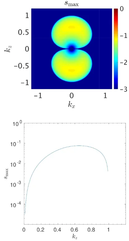
In Fig.2we illustrate the growth rate on the (kx,kz) plane (top panel), and for elevator modes as a function ofkz(bottom panel), for an example withS₌S_{/ =2.1, N}2

=N2_/ 2

=10, and Pr =10−2_{. The top panel shows that the fastest growing modes havekx} =0, and both panels demonstrate that the wavelength of the fastest growing mode (and that of the unstable modes in general, for these parameters) isO(d).

4 A N A L O G Y W I T H S A LT F I N G E R I N G F O R T H E A X I S Y M M E T R I C E Q UAT O R I A L G S F

In this section, we briefly reiterate the equivalence of the axisym-metric equatorial GSF instability at the equator with the well-studied salt fingering instability. This is helpful to understand the non-linear evolution of the instability, and allows us to check our axisymmetric simulations against the 2D simulations of salt fingering by e.g. Garaud & Brummell (2015). This analogy was first discussed by Goldreich & Schubert (1967) and demonstrated formally by Knobloch (1982). The non-linear equations governing

Figure 2. Top: base 10 logarithm of the growth rate of the axisymmetric GSF instability on the (kx,kz)-plane withS=2.1,N2=10, Pr=10−2. Bottom: growth rate of elevator modes on a logscale withkx=0 as a function ofkz. The top panel shows that the fastest growing modes at the equator havekx=0, and that these modes havekz=O(d−1).

the salt fingering instability for axisymmetric (y-invariant) flows are (e.g. Garaud2018), in dimensional form,

Dux_{= −}∂xp₊(θ₋μ)₊ν_∇2_{ux, (19)}

Duz_{= −}∂zp₊ν_∇2uz, (20)

Dθ _{= −}N2

ux₊κ_∇2θ, (21)

Dμ_{= −}N2

μux+κμ∇

2_{μ, (22)}

Duy₌ν_∇2uy, (23)

D₌∂t₊(ux∂x₊uz∂z), (24)

D

o

w

n

lo

a

d

e

d

fro

m

h

ttp

s:

//a

ca

d

e

mi

c.

o

u

p

.co

m/

mn

ra

s/

a

rt

icl

e

-a

b

st

ra

ct

/4

8

7

/2

/1

7

7

7

/5

4

9

2

2

6

9

b

y

U

n

ive

rsi

ty

o

f L

e

e

d

s

u

se

r

o

n

2

4

Ju

n

e

2

0

1

where we have taken the local gravity direction to be alongxto be consistent with our set-up in Section 2,μis the salinity (or heavy element content),N2

μis the background salinity (or heavy element) gradient, andκμ is the saline diffusivity (or diffusivity of heavy elements). Fory-invariant solutions,uy is passively advected and plays no role in the evolution of any instabilities.

For comparison, the evolution of the axisymmetric (y-invariant) equatorial GSF instability is governed by equations (1)–(4) (with ∂y₌0), i.e. by

Dux_{= −}∂xp₊(θ₊2uy)₊ν_∇2ux, (25)

Duz_{= −}∂zp₊ν_∇2_{uz, (26)}

Dθ _{= −}N2

ux₊κ_∇2θ, (27)

Duy_{= −}(2₋S)ux₊ν_∇2_{uy, (28)}

D₌∂t₊(ux∂x₊uz∂z), (29)

where these are written in dimensional form. This system is formally equivalent to equations (19)–(23) for fully non-linear axisymmetric solutions as long asκμ ₌ ν, and we also identify μ_{= −}2uy, andN2

μ=2(2−S)=κep2, so thatμrepresents an angular momentum stratification. The linear GSF instability is therefore also equivalent to salt fingering. However, it should be realized that for fully 3D (non-y-invariant) solutions, the non-linear equations describing salt fingering and GSF are no longer equivalent owing to the presence ofuyin the advection term. This means that while the axisymmetric evolution of both instabilities is formally identical (so we should obtain similar results to e.g. Garaud & Brummell 2015 and Xie, Julien & Knobloch 2019), the 3D evolution of the equatorial GSF instability differs from that of salt fingering.

5 N O N - L I N E A R R E S U LT S

We wish to explore the non-linear evolution of the instability and how this differs between axisymmetric and 3D simulations as a function of S, N2_{, Pr, and Ly (which can be used to probe the} importance of 3D effects). We also wish to analyse the efficiency of angular momentum transport, which is quantified by the Reynolds stressuxuy, where _· represents a volume average. An ‘effective viscosity’ can also be defined on dimensional grounds by the sum of the kinematic viscosity withνE, whereνE= 1_Suxuy, whether or not the turbulence acts in the manner of an eddy diffusion for angular momentum.

We initialize the flow using solenoidal random noise of amplitude 10−3_{for all wavenumbers in the range ˆi,j ,ˆ kˆ}

∈[1,21], wherekx₌ 2π

Lx

ˆ

i,ky₌ 2π

Ly

ˆ

j, andkz₌ 2π

Lz

ˆ

k. The domain size is chosen so thatLx =Lz₌100d, which is sufficient to contain several wavelengths of the fastest growing modes in each of our simulations.Lyis varied separately in the 3D simulations.

5.1 Illustrative axisymmetric simulations

We begin with a set of illustrative axisymmetric simulations with Pr₌ 10−2_,N2

=10, withS₌ 2.1 andS₌2.5. Note thatS>

2 is required for the shear flow to be centrifugally unstable in the absence of stratification, but that the flow is stable in the absence of thermal diffusion according to equation (16) (which would require S>7 for adiabatic axisymmetric instability).

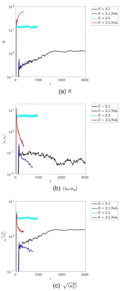
Fig. 3 shows the evolution of the volume-averaged kinetic energy K₌ 1_2|u_|2

(top panel), uxuy (top middle), the RMS latitudinal velocity vz₌

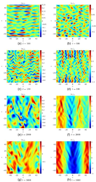
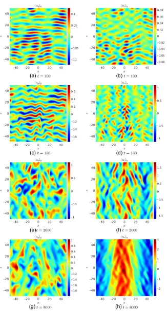
u2_{z (bottom middle), and minus the} radial buoyancy flux ₋uxθ, in simulations with S ₌ 2.1. The axisymmetric simulation is shown as the red line. This figure also shows the results from 3D simulations with various Ly, which will be discussed in Section 5.2. Snapshots of the y-averaged uy and uz velocity components in the (x, z)-plane at several times are shown in Fig.4 for the axisymmetric simulation with

S₌2.1.

After the initial saturation at t _∼ 130, there is a secondary growth of strong latitudinal shear flows (alongz), which quickly dominate the energy, as shown in the third panel of Fig. 3. The spatial structure of the flow is shown in the bottom two right-hand panels of Fig.4, which illustrates that these latitudinal flows possess significant radial (along x) shear. Following the development of these strong latitudinal shear flows, the angular momentum transport is significantly inhibited, and undergoes chaotic bursty dynamics, as is shown in the second panel of Fig.3.

The development of these strong latitudinal shear flows in an axisymmetric simulation is shown in snapshots at various times in Fig. 4, and as a Hovm¨oller diagram (y- andz-averageduz as a function ofxand t) in Fig.5. During the linear growth phase, att₌100,uy_∼uz, but shortly after the initial saturation,uzjets grow, and these jets merge until this component dominates. Byt ∼2000, the latitudinal shear flow persists in a configuration with two wavelengths in x, and strongly affects the radial propagation of finger-like motions, as can be seen fromuyin the bottom two left-hand panels. The latitudinal shear flow then merges to form a single wavelength in xbyt_∼4000, which further enhances the shear and reduces the angular momentum transport by shearing the radial fingers and reducing their radial extent. The buoyancy flux is also reduced when strong shears develop, which indicates that these jets act as barriers to transport, much like zonal flows (e.g. Diamond et al.2005).

The latitudinal shear flows are even more pronounced in sim-ulations with the stronger shear of S₌ 2.5. In Fig. 6we show the evolution of the same volume-averaged quantities as in Fig.3 for these simulations (with the axisymmetric case shown in red), along with comparison 3D simulations which will be described further in Section 5.2. The latitudinal flows in this simulation are not shown but are similar to those in Fig. 4except that they are stronger. Axisymmetric simulations exhibit bursty dynamics in which strong latitudinal jets inhibit instability in a cyclic manner reminiscent of predator-prey dynamics. This is similar to the effects of zonal flows driven by convection in a rotating annulus (e.g. Rotvig & Jones2006; Tobias, Oishi & Marston2018), and also those driven by the elliptical instability (e.g. Barker2016). Rapid cyclic transitions occur between a state with strong latitudinal jets and weak momentum transport, and a state with weaker latitudinal jets and stronger momentum transport. We have also explored cases with even stronger shears (S>2.5), and these behave in a qualitatively similar manner, except that larger Sleads to even more violent bursty dynamics.

Similar evolution, including the generation of latitudinal jets, has been observed in the analogous 2D salt fingering problem by Garaud & Brummell (2015), and also in an asymptotically reduced model of this system by Xie et al. (2019).

D

o

w

n

lo

a

d

e

d

fro

m

h

ttp

s:

//a

ca

d

e

mi

c.

o

u

p

.co

m/

mn

ra

s/

a

rt

icl

e

-a

b

st

ra

ct

/4

8

7

/2

/1

7

7

7

/5

4

9

2

2

6

9

b

y

U

n

ive

rsi

ty

o

f L

e

e

d

s

u

se

r

o

n

2

4

Ju

n

e

2

0

1

(a)

(b)

(c)

(d)

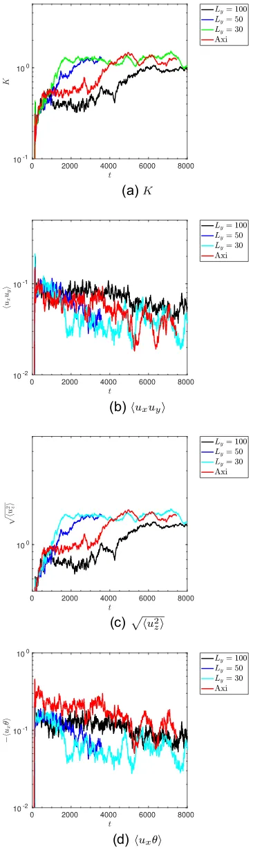
Figure 3. Temporal evolution ofK,uxuy,vz, and−uxθ, in a set of simulations withS=2.1,N2_{=10, Pr=10}−2_{, with various differentL}

y. The strong dependence onLyillustrates the importance of 3D effects on the non-linear evolution of the GSF instability.

5.2 Illustrative three-dimensional simulations

We now present 3D simulations with variousLyvalues with other-wise the same parameters as in Section 5.1 to explore the importance of 3D effects, and to explore whether the strong latitudinal shear flows are a robust feature. The importance of 3D effects can be seen in Fig.3, which shows the evolution of volume-averaged quantities for several 3D simulations withS₌2.1, where results withLy₌ 30, 50, and 100 can be compared with the axisymmetric simulation. Snapshots of the y-averaged uy and uz velocity components in the (x,z)-plane at several times are then shown in Fig.7for the 3D simulation withLy ₌100, which can be compared with the axisymmetric case in Fig.4.

The axisymmetric and 3D simulations behave similarly until just after the initial saturation of the instability. However, the subsequent evolution, including the generation of strong latitudinal shear flows, depends strongly onLy, and hence 3D effects are important. The axisymmetric simulations, and the 3D ones withLy₌30 and 50, exhibit much larger kinetic energies than the case withLy ₌100 untilt_∼4000, as is shown in the top panel of Fig.3. The time taken for latitudinal shear flows to grow is observed to depend onLy(and may also depend on the initial conditions).

The 3D simulation with Ly ₌ 100 behaves similarly to the axisymmetric simulation in the early non-linear phases, but byt ∼2000, it still hasuz_∼uy, and strong latitudinal jets are absent at this stage. The flow is instead closer to a homogeneous turbulence state. This is shown in snapshots at various times in Fig.7. The initial absence of strong latitudinal jets that advect and stretch the unstable motions in xleads to enhanced, and persistent, momentum (and buoyancy) transport relative to cases with smallerLy, as is shown in the second panel of Fig.3. However, the latitudinal jets do eventually develop in this example (and are shown in the bottom right-hand panel of Fig. 7), even if their effects on the flow are somewhat weaker than in the corresponding axisymmetric simulation.

The differences between axisymmetric and 3D simulations are much clearer in a set of simulations with a stronger shear ofS₌ 2.5. In Fig.6we show the evolution of the same volume-averaged quantities as Fig. 3for these simulations, which haveLy ₌ 30, 50, and 100. The y-averageduy and uz velocity components on the (x, z)-plane are shown att₌ 100 in Fig. 8. The instability now saturates in homogeneous turbulence in all 3D simulations for allLy considered. However, the energy level attained and the corresponding momentum transport does depend onLy, with a trend towards convergence forLy50.

The striking predator-prey-like dynamics observed in the axisym-metric simulation withS₌2.5 discussed in the previous section does not occur in three dimensions for any case withLy_≥30; jets are not observed even at longer times (though they would presumably also occur forS₌2.5 with small enoughLy). Presumably, strong latitudinal shears can only persist when they are stable to parasitic shear instabilities with long enough wavelengths alongy. Naively, we might expect a requirement onLyλxfor these strong shears to be suppressed, whereλxis the radial wavelength of the latitudinal shear flow.

The simulations in the previous section and this one highlight that the non-linear evolution can significantly differ between ax-isymmetric and 3D simulations. Axax-isymmetric simulations develop strong latitudinal jets whereas 3D simulations with large enoughLy prefer to saturate in homogeneous turbulence. This is reminiscent of the results of Garaud & Brummell (2015) for salt fingering. This is what we might have expected based on Section 4, but does not directly follow from the formal analogy presented there.

D

o

w

n

lo

a

d

e

d

fro

m

h

ttp

s:

//a

ca

d

e

mi

c.

o

u

p

.co

m/

mn

ra

s/

a

rt

icl

e

-a

b

st

ra

ct

/4

8

7

/2

/1

7

7

7

/5

4

9

2

2

6

9

b

y

U

n

ive

rsi

ty

o

f L

e

e

d

s

u

se

r

o

n

2

4

Ju

n

e

2

0

1

Figure 4. Snapshots ofy-averageduyanduzin the (x,z)-plane for an axisymmetric simulation withS=2.1,N2=10, Pr=10−2at various times. The top panels show the linear growing modes, which havekx∼0. The middle panels show the initial non-linear saturation, followed by the formation of latitudinal (alongz) jets. The bottom panels shows the strong latitudinal shear flows that have developed in the later stages, and their effects on the propagation of unstable finger-like motions inx.

D

o

w

n

lo

a

d

e

d

fro

m

h

ttp

s:

//a

ca

d

e

mi

c.

o

u

p

.co

m/

mn

ra

s/

a

rt

icl

e

-a

b

st

ra

ct

/4

8

7

/2

/1

7

7

7

/5

4

9

2

2

6

9

b

y

U

n

ive

rsi

ty

o

f L

e

e

d

s

u

se

r

o

n

2

4

Ju

n

e

2

0

1

Figure 5. Hovm¨oller diagram showing thex-averageduzvelocity compo-nent as a function ofxandt. This shows the formation and the merging of latitudinal jets in the axisymmetric simulation withS=2.1,N2_{=10, Pr=} 10−2_{, as also shown in Fig.4.}

We have also explored 3D cases with even stronger shears (S> 2.5), and these behave in a qualitatively similar manner – though see Section 5.4 for a further discussion of cases with very large S. Given that the anisotropy in axisymmetric simulations, or those with small domains alongy, is artificially imposed (rather than developing naturally from a more weakly constrained system), we advocate that 3D simulations withLx_∼Lz_∼Lyare likely to provide the most useful information regarding the non-linear evolution of the GSF instability in stars. Indeed, in real stars, there is no enforced azimuthal periodicity on a short length-scale, so cases in whichLyis large enough not to artificially constrain the flow are likely to be the most realistic. We will therefore focus on these simulations when we later consider the astrophysical consequences of our results. In addition, the formation of latitudinal jets is likely to be related to the adoption of periodic boundary conditions in the local latitudinal direction.

5.3 Comparison with simulations with stress-free boundaries inx

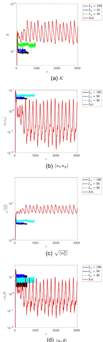
We will now briefly consider the effects of varying the boundary conditions on the non-linear evolution. To do this we have performed a pair of simulations with impenetrable, stress-free, fixed temper-ature boundary conditions. These conditions differ from shearing-periodic boundary conditions in two crucial ways: they allow the flow to modify the background shear flow even at the boundaries, and they also disallow elevator modes. We choosePr₌10−2_,N2 =10, andS₌2.1 andS₌2.5, and we also adoptLy₌30, since this requires the fewest number of grid points in total to resolve the flow.

In Fig.9we compare the evolution of volume-averaged quantities for a case with shearing-periodic, and one with stress-free, boundary conditions for each ofS₌2.1 andS₌2.5, respectively. Fig.10 shows corresponding snapshots of the flow in the (x,z)-plane for the case withS₌2.1. In Fig.9, the kinetic energy with stress-free impenetrable boundaries is observed to grow due to the generation of a stronguyflow which partially counteracts the imposed shear flow. The kinetic energy growth is just like with shearing-periodic boundaries, with the crucial difference that in this case the latitudinal

Figure 6. Temporal evolution ofK,uxuy,vz, and−uxθ, for a set of simulations withS=2.5,N2=10, Pr₌10−2_{with various differentL}

y. This clearly illustrates the importance of 3D effects on the non-linear evolution of the GSF instability.

D

o

w

n

lo

a

d

e

d

fro

m

h

ttp

s:

//a

ca

d

e

mi

c.

o

u

p

.co

m/

mn

ra

s/

a

rt

icl

e

-a

b

st

ra

ct

/4

8

7

/2

/1

7

7

7

/5

4

9

2

2

6

9

b

y

U

n

ive

rsi

ty

o

f L

e

e

d

s

u

se

r

o

n

2

4

Ju

n

e

2

0

1

Figure 7. Snapshots ofy-averageduyanduzin the (x,z)-plane for a 3D simulation withS=2.1,N2=10, Pr=10−2, andLy=100 at various times. This can be compared with the axisymmetric simulation in Fig.4and demonstrates that 3D effects can be important for the initial evolution, though in this case similar latitudinal jets eventually form.

D

o

w

n

lo

a

d

e

d

fro

m

h

ttp

s:

//a

ca

d

e

mi

c.

o

u

p

.co

m/

mn

ra

s/

a

rt

icl

e

-a

b

st

ra

ct

/4

8

7

/2

/1

7

7

7

/5

4

9

2

2

6

9

b

y

U

n

ive

rsi

ty

o

f L

e

e

d

s

u

se

r

o

n

2

4

Ju

n

e

2

0

1

Figure 8. Snapshots ofy-averageduyanduzin the (x,z)-plane for a 3D simulation withS=2.5,N2=10, Pr₌10−2_{, andL}

y=100 att=100 in the saturated quasi-homogeneous turbulent state. The flow is very different from the corresponding axisymmetric simulation, which is dominated by strong latitudinal jets much like those in Fig.4.

flow is in fact decreasing (bottom panel). The snapshots in Fig.10 also illustrate that a stronguyshear has developed byt_∼200, which gradually strengthens in time to dominate the flow byt_∼1000. The shear in the total (background₊perturbation) flow is now reduced by the action of the instability, relative to the initial imposed shear. However, note that this modification is still relatively weak even by t₌960, anduyyatx=0 is approximately only 1.5 per cent of the initial background shear velocity (₋105 atx₌0). Similar behaviour is found withS₌2.5, except that in this case the modification of the shear with these boundary conditions is then much stronger.

These simulations clearly demonstrate that the GSF instability produces angular momentum transport that reduces the overall differential rotation. This kind of modification of the imposed shear is not permitted by shearing-periodic boundary conditions, so these simulations highlight that the long-term evolution of the instability is dependent on the boundary conditions. However, the initial saturation level is similar, even if the longer term non-linear reduction of the total shear acts to reduce the momentum transport over time compared with the cases with shearing-periodic boundary conditions. The initial agreement between both sets of simulations indicates that we may continue to use shearing-periodic boundary conditions to probe the momentum transport, at least during the initial phases of homogeneous turbulence. In addition, since strong latitudinal jets are absent in simulations with impenetrable radial boundaries, this suggests that we should focus on the initial phases of homogeneous turbulence in our simulations with shearing-periodic boundaries when constructing a model to apply to astrophysics.

Figure 9. Comparison of the temporal evolution ofK,uxuy, andvz, for a 3D simulation with stress-free boundaries (labelled ‘Nek’) and shearing-periodic boundaries. The parameters areS₌2.1,N2

=10, Pr₌10−2_{, and} Ly=30. The energy with shearing-periodic boundaries grows due to the development of strong latitudinal shear flows, but in the case with stress-free impenetrable boundaries the energy instead grows due to the generation of a stronguyflow which counteracts the imposed shear.

5.4 Simulations with very large imposed shears

The non-linear behaviour described in Section 5.2 is typical of most of our simulations in which the GSF instability operates. However, we observe different behaviour whenSis very large. For our typical value ofN2

=10, note that whenS3, Ri₌N2_/S2_{1. For these} large shears, the shear dominates over the stable stratification and we might expect different non-linear evolution. Note also that ifS_≤ 7, the flow is linearly stable to adiabatic axisymmetric perturbations, so simulations in this regime are still probing the action of the GSF

D

o

w

n

lo

a

d

e

d

fro

m

h

ttp

s:

//a

ca

d

e

mi

c.

o

u

p

.co

m/

mn

ra

s/

a

rt

icl

e

-a

b

st

ra

ct

/4

8

7

/2

/1

7

7

7

/5

4

9

2

2

6

9

b

y

U

n

ive

rsi

ty

o

f L

e

e

d

s

u

se

r

o

n

2

4

Ju

n

e

2

0

1

Figure 10. Snapshots of y-averageduy in the (x, z)-plane from a 3D simulation with stress-free boundaries at two different times. The parameters areS₌2.1,N2

=10, Pr₌10−2_{, andL}

y=30. The stronguyflow is evident, which counteracts the imposed shear.

instability. Note that such large shears are probably not relevant in astrophysics, where we typically expect Ri_≫1 except very close to convection zones, but these simulations are nevertheless useful in allowing us to explore the non-linear behaviour in cases where we might expect the theory that we will present in the next section to no longer apply.

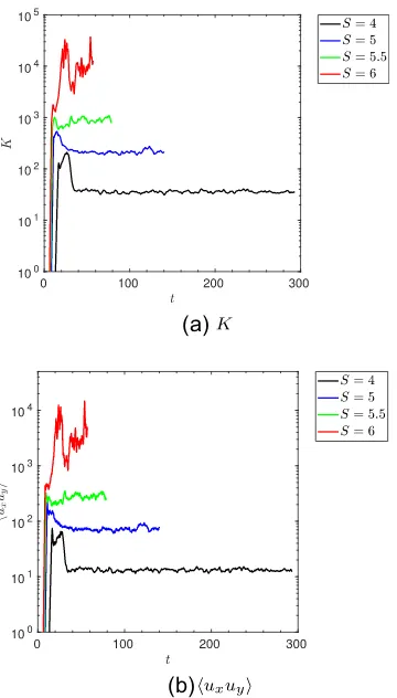
In this section, we use 3D simulations with shearing-periodic boundary conditions withPr₌0.1,N2

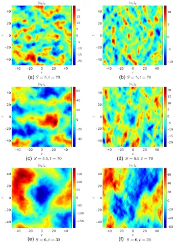
=10,Ly₌100, andS₌4, 5, 5.5, and 6 to illustrate the behaviour in these cases with strong shear. In Fig.11, we show the mean kinetic energy anduxuyas a function of time. Then, in Fig. 12, we show they-averageduy anduzflow components at a given time in the turbulent state in a simulation withS₌5, 5.5, and 6. We observe that the simulations withS_≤5.5 reach a statistically steady turbulent state with only small fluctuations about the mean kinetic energy and momentum transport. On the other hand, the simulation withS₌6 is strongly bursty, with large fluctuations in the kinetic energy and momentum transport. The flow corresponding to this simulation is shown in the bottom two panels of Fig.12, which shows the presence of large-scale flow structures in bothuy anduz. Fig.12shows that asSis increased, the flow saturates in large length-scale flows (which have also been found in salt fingering by e.g. Brown et al.2013, but not necessarily for the same reason).

Linear theory predicts that larger values ofSallow instability for increasingly larger wavelength modes, but this cannot be the

(a)

(b)

Figure 11. Temporal evolution ofKanduxuyfor a set of simulations with

N2_{=10, Pr=10}−1_,L

y=100, for the strong shear values ofS=4, 5, 5.5, and 6.

sole explanation for this behaviour. Indeed, the fastest growing mode has a wavelength of λz _≈ 9.3 (withkx ₌0) when S₌4, and λz _≈ 12.5 whenS ₌6, but the flow structures in the non-linear state are larger than this by more than a factor of 3 in the latter case. Hence, the formation of large-scale flows for large shears in likely to be related to the modification of the non-linear cascade when the shear dominates over the stratification. Due to their oscillatory nature, these large-scale flows may correspond with large-wavelength gravity waves, and they significantly enhance the transport over cases with smaller shears.

The formation of these large-scale flows is only observed for very strong shears, and such large shears are unlikely to be astrophysically relevant – the possible exception being very close to interface between the convective and radiative regions in very early phases of stellar evolution. Hence, we will not focus on explaining these simulations with large S, though we will note that they do saturate differently from those with smaller shears. This means that we would not expect the non-linear behaviour in simulations with largeSto be explained by a theory (such as the one that we will present in the next section) that is designed to explain simulations with smaller values ofS.

6 T H E O R Y F O R S AT U R AT I O N O F T H E G S F I N S TA B I L I T Y

For astrophysical applications we would like to quantify the angular momentum transport produced by the equatorial GSF instability. It is simplest to focus on developing a model for the saturation

D

o

w

n

lo

a

d

e

d

fro

m

h

ttp

s:

//a

ca

d

e

mi

c.

o

u

p

.co

m/

mn

ra

s/

a

rt

icl

e

-a

b

st

ra

ct

/4

8

7

/2

/1

7

7

7

/5

4

9

2

2

6

9

b

y

U

n

ive

rsi

ty

o

f L

e

e

d

s

u

se

r

o

n

2

4

Ju

n

e

2

0

1

Figure 12. Snapshots ofy-averageduyanduzin the (x,z)-plane for simulations with large shears, which illustrates the large-scale flows that develop. The parameters areN2=10, Pr₌10−1_,L

y=100, andS=5, 5.5, and 6, at the times indicated in the captions.

where the instability produces homogeneous turbulence, rather than coherent shear flows. As a result, our primary focus here is on explaining the non-linear behaviour in simulations withLx₌ Lz =Ly during the phases of homogeneous turbulence. A different (quasi-linear) theory (see e.g. Marston, Qi & Tobias2014) would be required to explain the behaviour in simulations where strong shear flows develop.

The simplest model of saturation of the equatorial instability is to assume that the flow is dominated by the fastest growing linear mode, and that this mode saturates when its growth rate balances its non-linear cascade rate. The basic idea is that the fastest growing modes predominantly involve radial (ux) flows with significant latitudinal (alongz) shear, and that parasitic shear instabilities acting on these flows would be expected to grow, and draw energy from

the primary mode, at a rate of orderkz_|ux_|. Note that the theory in this section will be expressed using dimensional quantities for clarity. We may expect saturation of the primary instability when

s_∼kzux. (30)

We define a constant of proportionalityA, which will be chosen later to fit our simulation data, through

ux_≡As

kz. (31)

For a single linear mode, equations (1)–(4) relate the perturbations by

uy₌ (S−2)

sν ux, (32)

D

o

w

n

lo

a

d

e

d

fro

m

h

ttp

s:

//a

ca

d

e

mi

c.

o

u

p

.co

m/

mn

ra

s/

a

rt

icl

e

-a

b

st

ra

ct

/4

8

7

/2

/1

7

7

7

/5

4

9

2

2

6

9

b

y

U

n

ive

rsi

ty

o

f L

e

e

d

s

u

se

r

o

n

2

4

Ju

n

e

2

0

1

uz _{= −}kx

kzux, (33)

θ ₌ −N

2

sκ ux, (34)

in terms of the radial velocityux, which is specified by equation (31). The corresponding time- and volume-averaged rates of momentum and heat transport, and the kinetic energy, for a single such mode are given by

uxuy ₌ (S−2)

2sν |ux| 2

, (35)

uyuz _{= −}(S−2)

2sν kx

kz|ux|

2_{, (36)}

uxuz _{= −}kx

2kz|ux|

2_{, (37)}

uxθ ₌ −N

2

2sκ |ux| 2

, (38)

1₂|u2

| = 1₄

1₊(S−2) 2

s2

ν

+ k

2 x

k2

z

|ux_|2. (39)

The values ofsandkzfor the fastest growing linear mode can be determined by solving equations (13) and (18).

This simple theory predicts the energy and momentum transport in terms of the properties of the linear instability and a single constantA, which is supposed to be independent of the parameters of our problem. However, with large values ofS, or when strong shear flows develop, we may expect the growth and cascade rates to be modified by the shear, so this theory would no longer be expected to hold, and a different type of theory would be needed (e.g. Bouchet, Nardini & Tangarife2013). We will determineAnumerically by fitting this model to our data from a suite of numerical simulations. Note that the model predicts uxuz ₌ uyuz ₌ 0 for ‘elevator modes’ withkx₌0. This theory is essentially equivalent to the ones proposed and tested for salt fingering by Denissenkov (2010) and Brown et al. (2013).

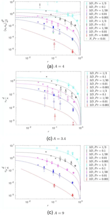
To test this theory we have performed a suite of simulations with the parameters listed in TableA1. We show the comparison of the theory and simulations foruxuyd2_/κ2_{versusr, where}

r₌

Pr Pr₋1

1₊ N 2

κ2

ep

, (40)

in the top panel of Fig. 13. Here all theoretical lines have been computed using the same value ofA₌4. We follow Brown et al. (2013) in definingrto map the region of parameter space that is unstable to the GSF instability tor_∈[0, 1]. Note that whenr_≥ 1, the system is stable to the GSF instability, and whenr<0, the system is unstable via the adiabatic Solberg–Høiland criterion, and that the supercriticality increases asr _→0. We have scaled the velocities in Figs13and14in units ofκ/d, rather thandas in the earlier figures. This separates the data with different Pr, and also aids the comparison with Fig.5of Brown et al. (2013) (which shows the heavy element transport by the salt fingering instability). The agreement is very good for most 3D simulations, indicating that this theory is essentially correct to explain the transport driven by the

Figure 13. Comparison between the theory (solid lines) presented in Section 6 and simulations (symbols) for several volume- and time-averaged quantities. 3D simulations are represented as crosses and axisymmetric simulations as open circles. The colours of each solid line and the symbols represent a given set of parameters, as identified in the legend. The panel captions represent the value ofAused in the theory, which was varied in the bottom two panels for a better fit. The top panel also shows the line Ri =1 as dotted lines, which indicates that the simulations that disagree with theory for smallrare those for which Ri1.

GSF instability. The agreement is also reasonable for 2D simulations for values ofrthat are not too smallr<0.1 or so. However, there is a departure from the theory for small values ofr, which corresponds with the large shear cases described in Section 5.4. The top panel shows the line Ri₌1 as dotted lines for the first three values of Pr. This indicates that the theory works well below this line, but fails to apply when Ri1, which lies above these lines.

In the middle and bottom panels of Fig.13, we also compare the theoretical predictions for the scaled RMS radial (vxd/κ₌

u2_{xd/κ) and azimuthal velocity (vyd/κ= u}2_{yd/κ). All}

D

o

w

n

lo

a

d

e

d

fro

m

h

ttp

s:

//a

ca

d

e

mi

c.

o

u

p

.co

m/

mn

ra

s/

a

rt

icl

e

-a

b

st

ra

ct

/4

8

7

/2

/1

7

7

7

/5

4

9

2

2

6

9

b

y

U

n

ive

rsi

ty

o

f L

e

e

d

s

u

se

r

o

n

2

4

Ju

n

e

2

0

1

(a)

(b)

Figure 14. Buoyancy flux−uxθand ‘turbulent Prandtl number’ PrE, compared with theory forA=4. Note that since we always have stable stratification, the buoyancy flux is negative.

curves use the same value ofA, but we have selected a different constant value to fit the data better, withA ₌ 3.4 forvx and A =9 forvy. The difference in the values of Arequired to fit the data for these quantities is presumably because the flow does not only consist of a single mode, but contains modes with severalkx andkz. In reality, the flow will consist of several modes, and the theory implicitly involves an integration over the domain, for which the spatial structure of the flow is important. As a result of the flow consisting of several modes, quantities that involve different products may require a different constant which accounts for this integration. Hence, we may not expect the sameAto be applicable for all quantities.

We note that we obtain enhanced transport and velocity ampli-tudes, not explained by our simple theory, for very large shears. For these simulations, Ri₌N2_/S2_{1, and the flow is no longer strongly} stratified. Those simulations are less relevant than those with larger rfor astrophysics, since we generally expect Ri₌N2_/S2

≫1 in

stellar radiation zones, though as noted previously, such cases may be relevant very near convection zones.

We have also calculateduxuz,uyuz, and the RMS latitudinal velocityvz. The theory would predict these quantities to be exactly zero because the fastest growing modes are elevator modes withkx =0. We observe them to be non-zero in general, but we confirm that they fluctuate about zero, consistent with theoretical expectations.

In Fig.14, we show the scaled buoyancy flux₋uxθd/κ, along with the theoretical predictions assumingA₌4. The agreement is very good apart from cases with smallr, just as withuxuy. The buoyancy flux in 3D simulations typically exceeds that in axisym-metric cases, presumably due to the presence of strong latitudinal shear flows that inhibit radial transport in the axisymmetric case.

We may also crudely define a ‘turbulent Prandtl number’ by:

PrE=

ν₊νE

κ₊κE =

ν₊ uxuy/S

κ_{+ |}uxθ/N2_| (41)

This is shown in the bottom panel of Fig. 14, and is found to depend on r, and is not a constant that is equal to the laminar Pr. Note that ν _≪ νE except whenr ∼ 1. We find that PrE ≤ 1 for all simulations performed. This indicates that the saturated state maintains an effective Prandtl number smaller than one, which supports further action of the GSF, rather than by saturating by increasing PrE>1, which would eliminate GSF.

6.1 The absence of ‘layering’ by the GSF instability

Salt fingering in the oceans is known to produce layering of the density field, leading to the formation of density staircases, in which convective layers are separated by thin diffusive interfaces. The presence of layering is associated with a significant enhancement in the rates of turbulent transport over that of a homogeneous turbulent medium. For low Pr fluids, Brown et al. (2013) showed that layer formation is possible by the salt fingering instability by the ‘collective instability’ (which involves the excitation of large-scale gravity waves that form layers when the waves break), but not by the linear mean-field ‘γ-instability’ of Radko (2003) and Traxler et al. (2011). Theγ-instability involves slow-growing, horizontally invariant but vertically varying modes. Both of these are secondary instabilities that are driven by a positive feedback mechanism between large-scale temperature and salinity perturbations, and the turbulent fluxes induced by them, which can be derived within a mean-field framework. Given the potential importance of such layering for turbulent transport, we wish to determine whether layering of the angular momentum field by the GSF instability may be possible. In our simulations at the equator we do not observe layering inuy. Instead, we observe the formation ofuzjets, which is not what we are attempting to explain here. In this section we are interested in exploring whether the absence of observed layering in uyis consistent with mean-field theories that have been tested for the related salt fingering problem. This is motivated by the analogy discussed in Section 4.

In order to explore whether the GSF instability would be expected to produce such layering i.e. generate mean flows inuythat vary in x, we can calculate whether the mean-fieldγ-instability may occur. Given that the axisymmetric problem is equivalent to salt fingering, by analogy with that problem, we may define the ‘density ratio’

R0₌ N

2

−κ2

ep

. (42)

The ratio of turbulent buoyancy flux to angular momentum flux is

γ ₌ (κN

2

− uxθ)

−νκ2

ep+2uxuy

. (43)

If this is a monotonically increasing function ofR0, the mean-field γ-instability is unable to produce ‘layering’ ofuyflows alongzthat vary inx. In Fig.15, we plotγ as a function ofR0. This clearly indicates that for the parameters considered, layering cannot occur via theγ-instability for the equatorial GSF instability. The smallest values of R0 for Pr₌ 0.1 are slightly non-monotonic, but still increasing withR0. This is consistent with the absence of layering in our simulations. These results are similar to those of Brown et al. (2013) for salt fingering.

However, as we have discussed in Section 5.4, we do observe the excitation of large-scale flows that may correspond with gravity

D

o

w

n

lo

a

d

e

d

fro

m

h

ttp

s:

//a

ca

d

e

mi

c.

o

u

p

.co

m/

mn

ra

s/

a

rt

icl

e

-a

b

st

ra

ct

/4

8

7

/2

/1

7

7

7

/5

4

9

2

2

6

9

b

y

U

n

ive

rsi

ty

o

f L

e

e

d

s

u

se

r

o

n

2

4

Ju

n

e

2

0

1