Computational model of MST neuron receptive field and interaction effect for the perception of self-motion

Rochester Institute of Technology

RIT Scholar Works

Theses Thesis/Dissertation Collections

2008

Computational model of MST neuron receptive

field and interaction effect for the perception of

self-motion

Chen-Ping Yu

Follow this and additional works at:http://scholarworks.rit.edu/theses

This Thesis is brought to you for free and open access by the Thesis/Dissertation Collections at RIT Scholar Works. It has been accepted for inclusion in Theses by an authorized administrator of RIT Scholar Works. For more information, please [email protected].

Recommended Citation

Computational model of MST neuron receptive field and

interaction effect for the perception of self-motion

A Thesis Submitted in Partial Fulfillment of the Requirements for the Degree of

Master of Science in Computer Science

by

Chen-Ping Yu

[email protected]

Submitted to the Department of Computer Science

Rochester Institute of Technology

July 21, 2008

Approved by Committee Members:

Dr. Roger Gaborski, RIT

Chairman

Drs. Charles Duffy, U. of Rochester

Reader

1

Abstract

Biologically plausible approach is an alternative to conventional engineering approaches

when developing algorithms for intelligent systems. It is apparent that biologically inspired

algorithms may yield more expensive calculations when comparing its run time to the more

commonly used engineering algorithms. However, biologically inspired approaches have great

potential in generating better and more accurate outputs as healthy human brains. Therefore more

and more new and exciting researches are being experimented everyday in hope to develop better

models of our brain that can be utilized by the machines.

This thesis work is an effort to design and implement a computational model of neurons

from the visual cortex’s MST area (medial superior temporal area). MST’s primary responsibility

is detecting self-motion from optic flow stimulus that are segmented from the visual input. The

computational models are to be built with dual Gaussian functions and genetic algorithm as its

principle training method, from the data collected through lab monkey’s MST neurons. The

resulting computational models can be used in further researches as part of motion detection

mechanism by machine vision applications, which may prove to be an effective alternative

motion detection algorithm in contrast to the conventional computer vision algorithms such as

frame differencing. This thesis work will also explore the interaction effect that has been

discovered from the newly gathered data, provided by University of Rochester Medical Center,

2

Table of Contents

1. Introduction...5

2. Background ...10

2.1. Retina ...10

2.2. Receptive Fields ...12

2.3. Primary Visual Cortex (V1) ...14

2.4. Ventral and Dorsal Stream (“what” and “where” pathway) ...16

2.5. Ventral Steam (the “what” pathway) ...17

2.6. Dorsal Stream (the “where” pathway) ...19

2.7. MST and Optic Flow...22

3. Data ...24

3.1. Neurophysiological Stimuli...24

3.2. Neuron Recording ...27

3.3. Singles Data...28

3.4. Optic Flow Data ...34

3.5. Doubles Data ...37

3.6. Interaction Effects in Doubles Recordings...40

4. Methods...44

4.1. Training of the Dual Gaussian Model ...44

4.1.1. Dual Gaussian Singles Models ...44

4.1.2. Clamping ...46

4.2. Genetic Algorithm – Singles Model Training...47

3

4.2.2. Selection ...48

4.2.3. Crossover...51

4.2.4. Mutation ...52

4.3. Genetic Algorithm – Doubles Model Training ...54

4.3.1. Dual Gaussian Doubles Model and Template-Matching ...54

4.3.2. Doubles Diagonal Hotspot Data Interpolation ...57

4.4. Gain Modulation ...59

4.4.1. Nine Gain Factors...59

4.4.2. Eighteen Gain Factors ...60

4.5. Optic Flow Prediction ...60

4.5.1. Singles to Flow Prediction...61

4.5.2. Template Matching Flow Prediction with Doubles Dual Gaussian Models ...62

4.5.3. X and O Doubles Template ...63

5. Results ...65

5.1. Singles Model...65

5.2. Doubles Model ...70

5.3. Flow Prediction ...76

5.3.1. Singles to Flow Prediction...76

5.3.2. Doubles to Flow Prediction ...81

5.3.3. Singles Gain Modulation – 9 Gain Factors ...86

5.3.4. Singles Gain Modulation – 18 Gain Factors ...92

5.4. Performance Comparisons ...98

5.4.1. Singles vs Doubles in Flow Prediction...98

5.4.2. Doubles Model with Interaction Effects...103

4

6. Summary and Conclusion ...113

7. Future Work...116

5

1. Introduction

The human brain excels in just about every aspect of function as an intelligent system.

Therefore, biologically inspired systems attempt to base its designs from the organization and the

functionalities of the human brain. This thesis work is an effort to design and implement a

computational model of neurons from the visual cortex’s MST area (medial superior temporal

area), with dual Gaussian receptive field functions derived by a GA as its principle training

method My goal is to fit the data collected in awake monkey neurophysiological studies of MST

neurons, and to better understand the receptive field mechanisms of their role in the visual

motion processing of optic flow stimuli.

The results of the computational models of this thesis will bring us closer to developing a

better biologically feasible computer vision system. However, due to the fundamental differences

between the computational algorithms and the brain's neuronal format, it is difficult to implement

biologically feasible algorithms and systems with many computational approaches. Another

obstacle is that we do not currently have enough understanding of how the brain process visual

information. As we make progress toward understanding the brain in greater detail, we will be

able to develop better and more accurate models for specific parts of the brain. These new

understandings can then be utilized onto machine algorithms that are more biologically plausible.

The criterion of biologically plausibility is an alternative to conventional engineering

approaches when developing algorithms for intelligent systems. It is apparent that biologically

inspired algorithms may yield more expensive calculations when comparing its run time to the

more commonly used engineering algorithms. However, biologically inspired approaches have

6

healthy human brain. Therefore more and more new and exciting research is being developed in

hope of creating the foundation for better models of our brain that can be implemented in

machines.

Computer vision, being a branch of the field of artificial intelligence, is one of the areas

that may benefit greatly from new understandings of biological vision. Approaches include

Gaussian derivative models for motion related detections that are based on the receptive fields of

visual cortex neurons and are able to sense the movement of objects across multiple display

frames [22]. Dr. Young has done extensive research in regards to biologically plausible models of

the visual cortex. His models of Gaussian derivatives mimic the center-surround receptive field

organization of visual cortical neurons. By taking more derivatives of Gaussian curves, it is

possible to create various different models that contain different lobes, phase, directions, and

frequencies. Using these Gaussian derivatives he was able to create models that detect basic

moving edges, as well as cars moving on the highway. The Gaussian derivative models also has

great potential to be used in many different motion sensing applications such as surveillance

cameras and object tracking systems.

There is also modeling effort done in the higher level of the visual cortex. VisNet is one

such example [18]. VisNet focuses on the modeling of connections between neurons within

visual cortex, rather than single neuron's receptive field representations. VistNet is a network of

nodes interconnected in a hierarchical format. The nodes are initially generated with random

connections, and it is a supervised network which is trained with its training set, with Bayesian

probabilistic learning rules that either keep or cut off connections between nodes. The trained

VisNet model can be used as pattern recognition systems, or object recognition applications.

7

contribute as biologically inspired models that can be used in machine vision systems. Gaussian

derivative models [22] are included in this category since their development was based on the

neuron's center-surround receptive field organization [14]. There are also models developed

based on the MT (medial temporal) area of the visual cortex that is analyzed to understand how

the MT neurons can sense motion of visual pattern [19].

Thus, computational neuroscience models includes single neuron models, sensory

processing models, neuron organization models such as VisNet [18], and models of higher

cognitive function, learning, and consciousness. This thesis work focuses on single neuron

contributions of visual motion sensory processing. The work may be used in future machine

vision applications that are related to motion processing as biologically inspired computer vision

systems. Specifically, this thesis work is aimed at developing receptive field models of MST

neurons with discovered interaction effects that may account for flow selectivity in some neurons

[24]. The interaction dependent changes in selectivity can be as dramatic as reversing the

direction of visual motion preferences. To model these effects, recorded firing rates from

neurophysiological studies of interactions between local motion stimuli will be trained into the

MST receptive field models. The interaction effects will be tested to determine whether they

allow the models to mimic the neurons optic flow selectivity by shifting local motion selectivity

according to specific combinations of local-motion across a neuron’s receptive field.

Understanding the pathway of visual information processing enables future research

efforts related to biologically inspired machine vision systems. At the highest level, we all accept

that the eyes receive light that is reflected from the objects around us. The retina transduces that

light to create a neuronal signal that it relays through the optic nerve, then the thalamic lateral

8

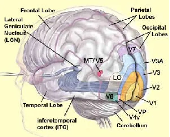
Figure 1 from McGill U. Website, Canada

From V1, visual information splits into two parallel steams of processing: the ventral

stream, also known as the what pathway, and the dorsal stream, also known as the where

pathway (Figure 2). The ventral stream goes from V1 to V2, V4, then IT (inferior temporal area).

This pathway is called the what pathway because it mainly detects and recognizes objects from

the visual information. The dorsal stream goes from V1 to V2, MT (medial temporal area), then

MST. This pathway is called the where pathway due to its ability to process object’s motion in

the scene, as well as self-motion. The combination of these two information processing steams in

parallel results in the precise understanding of what we see.

Some further details of each area and each process pathway will be explained in the next

section. In addition, basic receptive field properties and features of the optic flow that is seen

during self-motion will also be discussed in greater length in the next section as they are the

9

Figure 2 The Visual Pathway, from McGill University Website, Canada

10

2. Background

Before the details of any neuronal modeling effort can be understood, it is essential to

have some agreed upon description of the basic architecture of the brain systems to be

considered. Since this research is on modeling the receptive field properties of MST neurons, and

interactions between segments of MST neuronal receptive fields, it is important to be aware of

how the human brain processes the visual input received from the eyes.

2.1. Retina

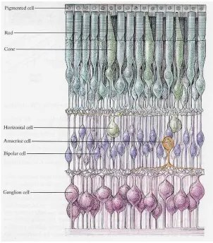
The retina is at the back of the eye and contains several layers of cells that allow us to

process color and light intensities [11]. The retina includes layers of ganglion cells, bipolar cells,

horizontal cell, rods, and cones (Figure 3).

11

Although the ganglion cells are closest to the iris, the light that passes through the cornea

would pass through all the layers of ganglion cells and bipolar cells, and be received by the rods

and cones first, then the input information is propagated to bipolar cells, ganglion cells, then

along the optic nerve to the visual cortex at the back of the brain [11].

The rods are responsible in processing input information in low ambient light intensity

conditions; the cones process color input at higher light intensity conditions [11]. Rods are also

in a much larger numbers compared to the cones in the retina, there are approximately 100

million rods as comparing to just 5 million cones in our retina. However, our fovea, which is

where we see the most detail with our central vision, contains mostly cones.

12

Rods and cones output to the bipolar cells. The bipolar cell’s effective responsibility is to

transfer the visual information from the rods and cones to the ganglion cells. The ganglion cells,

which converts the light information into action potentials, fires spikes and outputs to the lateral

geniculate nucleus (LGN), which acts as a relay station for the information inputs [11]. Since the

LGN receives more than just visual information, but also inputs from the cerebral cortex, and the

brainstem, LGN may filter visual information before passing it on to primary visual cortex. In

particular, both the left and right LGN receives visual input from both eyes. This allows the LGN

to send the image of the contra-lateral visual field (opposite side of the visual world) from both

eyes to the primary visual cortex on its side.

2.2. Receptive Fields

Before going further into how visual information is processed in visual cortex, we will

consider the basic design of the neuronal receptive fields that supply information to visual

cortex. The receptive fields of retinal ganglion cells and LGN neurons share the same basic

design. This design is that of the center-surround structured receptive field [14]. This structure is

of two basic varieties: on-center off-surround, and off-center on-surround (Figure 5).

Figure 5 Left: on-center off-surround receptive field

13

When an on-center segment is illuminated it makes the neuron fire more, when an

off-surround segment is illuminated it makes the neuron fire less [11]. Likewise, when the

illumination of an on-center segment is extinguished the neuron fires less. When the illumination

of and off-surround segment is extinguished the neuron fires more. The opposite scenario applies

with off-center on-surround retinal or LGN receptive fields.

The center-surround organization of many retinal and LGN receptive fields has been

thought to be combined to create the various types of receptive field organizations found in V1

cortex. Consider that if such center-surround receptive fields arranged along a straight line

through the visual field their outputs could be combined to create an orientation selective V1

receptive field [11]. If such a cell is organized to be sensitive with a 90 degrees straight line in

sight, then when the 90 degrees straight line is within the center of the receptive field, the cell

would fire its output very frequently, as in an excitatory action. However if the straight line is

perceived at where the surrounding of the receptive field is, then the cell would inhibit its firing

of signal, as in an inhibitory action. The off-center on-surround acts similarly as the example,

just in an opposite way. This is one theory of the orientation selectivity of V1 simple cells

14

Figure 6 Orientation specificity of V1 simple cell receptive field, white bar

is the stimuli. When the white bar is at different orientation in the receptive

field, the cell reacts differently. Figure from Hubel, 1995.

2.3. Primary Visual Cortex (V1)

The primary visual cortex, anatomically known as the striate cortex due to white matter

stripe through layer IV, is also labeled as V1 to refer to its functional role as first visual

processing stage after the LGN. V1 is part of the occipital lobe occupying the posterior tip of the

brain. A diverse assortment of neurons in V1 are designated simple cells (for having separate

excitatory and inhibitory subfields), complex cells (for their inseparable subfields), and

hypercomplex (for end-stop inhibition to long bar stimuli) [11]. All of these cells are higher up in

their processing of visual information than retinal and LGN center-surround cells. The receptive

fields of V1 simple, complex, and hypercomplex have been thought to be composed of a

15

Figure 7 LGN projection to V1, from Hubel, “Eye, Brain, and

Vision.” 1995.

Figure 7 presents a diagram of the inferior view of the human brain, looking from straight

below the brain up into the brain. V1 is at the bottom in this drawing, where it is labeled as

primary visual cortex. Each half of the brain, a hemisphere, contains half of V1. V1 is the first

major processing stage for the analysis of visual information. In addition to the diverse receptive

field properties of V1 cortex, these neurons are also responsive to color and movements in the

visual field, as well as some pattern. However, for the detailed and precise processing of the

visual input, V1 splits its output information into two somewhat distinctive visual processing

16

Figure 8 Blue: Primary Visual Cortex (V1)

Purple: Ventral steam

Green: Dorsal steam

figure from Wikipedia.com, “Dorsal Stream”

2.4. Ventral and Dorsal Stream (“what” and “where” pathway)

As the primary visual cortex, V1, receives the spikes of action potential firing from the

LGN, the information processing starts to split into two parallel processing stream: the ventral

stream and the dorsal stream (Figure 8). The ventral stream processes the objects seen in the

scene and detects what they are, whereas the dorsal stream processes object locations and motion

as well as the full-field motion that results from the observer’s self-motion (optic flow) [11].

The path of information flow in the ventral stream takes place in the sequence of areas

from V1, to V2, to V4, and then to IT. The path of information flow in the dorsal stream takes

place in the sequence of areas from V1, to V2, to MT, and then to MST. Both streams share the

17

is responsible for some color and directional selectivity [11]. V4 is not part of the dorsal stream

because V4’s major functionality is in processing color. Color information is more important

when recognizing objects but much less important when determining the movement or the speed

of something that is in motion. In fact, all we need is the light intensity (black/white) to

determine objects’ motions and self-motion, therefore it makes a lot of sense for dorsal stream,

which detects motion, to go past the V4 processing of color, while the ventral stream gets the

color information to further determine all the objects from the visual scene (Figure 9).

Figure 9, the dorsal and ventral stream.

2.5. Ventral Stream (the “What” pathway)

The ventral stream, which is indicated as the purple blocks along the bottom in figure 9,

represents temporal lobe processing of visual data from V1 in parallel with dorsal stream area

shown as green blocks. The ventral stream is mostly responsible for object and pattern

recognition and identification; therefore it importantly accesses and contributes to long term

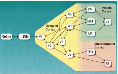
18 V4, and IT (Figure 10).

Figure 10, the information flow through dorsal stream extrastriate visual cortical areas.

V1 is, as described earlier, sensitive to color and directional selective stimulus. V2 and

V4 share very similar functionalities in terms of color detection and complex cell directional

selectivity as V1 [11]. However, as the processing level goes higher and deeper from V1 to V4

then to IT (inferior temporal area), some research indicates that the attentional modulation of

neuronal response sensitivities become stronger at the higher stages, although there remains a

great deal of disagreement on this point. V4 primarily processes color and shape information,

therefore IT has very complex receptive fields due to the large amount of processed information

and visual area from the processing of V1 through V4.

Common biologically inspired object detection algorithms that mimic how ventral steam

processes shape and color information utilize Gabor filters [20]. Gabor filters with different

angles of orientation are able to smooth the image, and filter for a specific orientation by

convolution with shaped filter at various angles. For example, applying a Gabor filter that is at

19

Figure 11, Gabor Filter 90° (left) convolved with a grey scale image (middle). Result (right)

shows the vertical (90°) edges displaying higher intensity (darker areas) than non-vertical

parts of the image (lighter areas).

This type of Gabor filter smoothing is very useful for object recognition algorithms that

are biologically inspired. By setting up and getting the responses of multiple Gabor filters with

different orientation at different locations of an input image, we are able to segment for specific

shape of objects from the responses generated [20]. We can also obtain the original color values

of the segmented area from the Gabor filters, which help represent the object segmented with

more information, therefore completing the ventral-stream inspired object detection algorithm.

2.6. Dorsal Steam (the “Where” pathway)

The dorsal stream, which is indicated as the green blocks along the top in figure 8

represents V1 occipital lobe projections toward the parietal lobe of the brain. The dorsal stream

process visual motion data from V1 in parallel with the ventral stream’s processing object

features. The dorsal stream is mostly responsible for spatial understanding, which recognizes

20

Figure 12, the information flow through dorsal stream extrastriate visual cortical areas.

From V2, the ventral stream continues into V4 for more color processing as stated from

the earlier section. The dorsal stream, however, continues into MT (Medial Temporal area) after

the basic edge and color processing done from V1 and V2. MT area is responsible for

recognizing where objects are located in the scene. As the objects move or as we move, MT

keeps us updated with respect to where objects are, therefore enabling us to detect motion over

time. Motion detection in general does not require color information about the object, this may

be related to the fact that a person isn’t able to detect the color and shape details about a car

passing by very quickly, but is able to sense that some object was moving though their visual

field. MST (Medial Superior Temporal area), being another processing stage after MT,

specifically detects the visual motion patterns that result from observer self-motion [4]. These

patterns of visual motion from self-motion are referred to as optic flow, which is represented in

cortical area MST, which also does not require color information.

Dorsal stream’s motion detection processing in MT can be simulated with Gaussian

derivative models developed by Dr. Richard Young [22]. A 3-dimentional Gaussian derivative

model that is convoluted with an input video is able to detect moving objects with time as its 3rd

axis. By generating the GD model with different orientation, it is able to respond to different

21

Figure 13, 3-Dimentional Gaussian Derivative Models. G00 as Gaussian function, G10

being the first derivative of Gaussian, G20 being the 2nd derivative. Figure from Young,

2001.

As the GD model is rotated with respect to Y axis, convolved with each time frame of the

GD model with every frame from the video of interest sequentially, if any object or edge is

moving in similar direction as the rotated GD’s orientation, the GD model will respond with

22

2.7. MST and Optic Flow

MST is the next stage of dorsal stream processing after MT. MST is responsible for

self-motion detection from optic flow and the neural representation of that visual self-motion information.

Due to being aware of self-motion, a person is able to estimate his heading direction and avoid

obstacles even during relatively fast motion through the environment.

Optic flow is the visual input that MST utilizes to process and determine heading

direction during self-motion (Figure 14). Optic flow is the radial pattern of visual motion that is

created by a person’s self-motion. It contains a focus of expansion from which all movement

appears to emanate. The focus of expansion (FOE), the singularity where the optic flow cues

flow out from, indicates the person’s heading direction under most circumstances [15]. By

processing optic flow, we are able to navigate around in an environment very efficiently without

the need of knowing the details of our surrounding objects, except knowing their location and

their relative motion. Optic flow is commonly simulated as being black and white, and these

stimuli appear to activate MST neurons effectively, suggesting that the processing of color

information is independent at this stage, as is consistent with the dual pathways model described

above [4]. MST’s representation of visual motion information is so useful that the airplane pilots

land the planes with optic flow assisted screen to guide the landing more accurately with ease by

23

Adapted from Gibson (1950) Adapted from Gibson (1950)

Figure 14, optic flow of a pilot landing its plane.

MST neurons mainly process optic flow representation of our visual input. It is also the

next processing level after MT, therefore it is not surprising that its neurons appear to have very

complex receptive fields due to its high level of visual motion processing. MST neurons’

receptive fields are conventionally known as solid state much like other motion sensitive neurons

– the responses of firing rate can be summed up from local motions responses, and it does not

alter its tuning of flow selectivity. However, our data reveals interesting findings in which our

MST neurons shift its flow selectivity with different optic flow stimuli, sometimes even reversed

from its local-motion selectivity. This effect will be discussed and displayed in more details in

24

3. Data

3.1. Neurophysiological Stimuli

The neurophysiological data used in this thesis were collected at University of Rochester

Medical Center, Cognitive Neuroscience Laboratory by Drs. Charles Duffy and David Logan

with subsequent data management overseen by Dr. William Page. In brief, the responses of

single neurons were recorded from the dorsal segment of the medial superior temporal area

(MSTd) in the cerebral hemispheres of adult Rhesus monkeys. Surgical preparation began with

sedation followed by venous catheterization, endotracheal intubation, and general anesthesia

using inhaled isoflurane. Scleral search coils were implanted around the limbus in both eyes [13]

to monitor eye position using the magnetic search coil technique [16]. A head holder and bilateral

recording cylinders were placed over 2 cm trephine holes centered above area MSTd.

Postoperative analgesia with banamine was administered in consultation with the veterinary

staff. All protocols were approved by the University of Rochester Committee on Animal

Research and complied with Public Health Service and Society for Neuroscience policy on

laboratory animals.

The monkeys were trained to sit in a primate chair and perform a visual fixation task. All

stimulus presentation trials began with the illumination of a stationary, red fixation point

centered on the tangent screen (Figure14). If the monkey maintained fixation (+/-3o) throughout

the 5-second trial, an auditory tone was sounded and liquid reward was dispensed. Recording

sessions were begun after the animal consistently completed trials with an accuracy of >90%.

25

ECP4100) at 60 Hz to cover the central visual field (90° x 90°) unless otherwise specified.

The monkey maintained visual fixation on a tangent screen during the presentation of all

visual stimuli. The display screen is a 90° x 90° rear-projection screen that is 48 cm in front of

the monkey. In experiments in which local motion stimuli were presented, the projection was

sub-divided into a three by three array (Figure 14). Dividing the viewing area into these nine

segments helps localize difference in response when local motion occurs at different places in the

visual field. This also allows the possibility of multiple segments combination testing. The nine

segments are labeled for implementation usage as follows:

Figure 15, a stationed monkey fixated at the center of the screen as

indicated by the red dot. The screen is divided into 3x3 sections

as the white division lines indicates (there is no real division line

26

After the monkey fixating at the center of the screen for 500 ms, a 2 second block of

motion stimuli was presented. Each block contains 4 different motion stimuli, with each motion

stimuli being displayed for 500 ms. The baseline firing rate of a neuron is recorded during the

500 ms fixation interval for each block, and the neuron’s firing rate from each stimuli block is

averaged over 6 trials of presentation.

Visual motion stimuli are made up of 500 white dots moving toward 1 of the 4 cardinal

planar direction on the black background for singles and doubles experiments, while the motion

stimuli for optic flow experiment contains a set of 16 global flow motions. Each dot encloses

0.19° at 2.61 cd/m² against a 0.18 cd/m² background. Each dots’ initial position is randomly

generated in the first frame with random life of 1 – 60 frames in each stimulus. Dots accelerate

as a sine x cosine function of their distance from the FOE, maintaining an average speed of

40°/s.

According to different experiments, the display screen may have one or more segments of

the 3 by 3 square showing dots moving to one of the eight directions: 0 degrees, 45 degrees, 90

degrees, 135 degrees, 180 degrees, 225 degrees, 270 degrees, and 315 degrees (Figure 15). In the

data sheet, they are labeled as integers 1 to 8 as to indicate motion 0° to 315°.

Figure 16, the eight different directions of motion that white dots may be displaying on

segments of the screen. From left to right: 0°, 45°, 90°, 135°, 180°, 225°, 270°, and 315°.

27

(“singles” experiment), there may be a combination of 2 patches showing the same or different

motions of dots (“doubles” experiment), and all 9 segments may also be fully displaying the

moving dots (“optic flow” experiment). The specifics depend on which experiment is being run

at the moment. During each 2 sec motion stimuli presentation block, the singles and doubles

stimuli were randomly interleaved in either the “X” or “O” pattern (Figure 16). The sequence of

testing is repeated until all stimuli were tested. The optic flow motion stimuli was tested on its

own without interleaving any other type of stimuli, and the optic flow motion stimuli contains 16

different full screen motion consists of white dots moving on the black background (Figure 21).

3.2. Neuron Recording

Microelectrode penetrations were made using epoxy-coated tungsten microelectrodes

(Microprobe) that were passed into cortex through a transdural guide tube positioned within the

recording cylinder [3]. Neural activity was monitored to locate the depth of physiological

landmarks, and experiments were initiated whenever neuronal discharges were clearly isolated.

Single neuron discharges were isolated using a dual window discriminator and stored with the

stimulus and behavioral event markers using the REX experimental control system [10]. Neuron

firing data were averaged across the 500 ms period of six to eight stimulus presentations to

characterize responses to each stimulus. When a neuron was isolated, we used a hand-held

projector to define its approximate receptive field boundaries. We used physiological criteria for

identifying MST neurons including their having large receptive fields (>20x20°), which contain

the fixation point, with direction-selective responses, preferring large moving patterns rather than

28

penetration across the superior temporal sulcus (STS) to identify the responses of MT neurons.

MT was identified as having much smaller receptive fields that are proportionate to the

eccentricity of the receptive field center and show greater responsiveness to bar or spot

movement than is seen in MST.

The stereotaxic positioning of the recording chambers and the depths of microelectrode

penetrations direct neuron recordings into cortical area MST. During the course of these

experiments, microelectrode positioning in MST was confirmed by magnetic resonance imaging

of the brain with microelectrodes in place. Images were obtained in the sagittal plane on a 1.5

Tesla magnet (General Electric) with fast spoiled gradient echo technique (TR = 23.5, TE = 10.3,

30° flip angle). The MR scans confirmed the location of the electrode tips in the anterior bank of

the STS. At the end of experiments on a monkey, electrolytic marks (25 µA x 25 s) were made

along the penetration tracks in three guide tubes in each hemisphere. After perfusing the animal

and fixing the tissue, posterior cortical blocks were cut in 50-mm thick sections. Every fourth

and fifth section was stained by the Nissl and Luxol Fast blue methods, respectively. The

electrolytic lesions were identified relative to anatomic landmarks to extrapolate the position of

the recording sites.

3.3. Singles Data

The singles data were collected by displaying motion in one of the nine patches at a time

for 500 ms. Each testing neuron receives two possible sets of input combinations: X or O type of

segment combinations (Figure 16). If a neuron is being tested for an X combination, the neuron

29

experiment displays motion at four segments one at a time: segment 2, 4, 6, and 8 (Figure 19).

Figure 17, the integer label for each segment of the screen. The X pattern of testing will test

only segment 1, 3, 5, 7, which looks like the character X (red labels), while the O pattern of

testing will test only segment 2, 4, 6, 8, which looks like the character O (white labels).

Each segment of testing includes four planar directions of motion: 0 degrees, 90 degrees,

180 degrees, and 270 degrees. Therefore, the X testing pattern would result in 20 entries of

30

Figure 18, the X pattern of Singles experiment. From left top to right bottom: Segment 1

displays the 4 planar motion (0°, 90°, 180°, 270°) for 4 separate recordings, then recording

31

0.333333 1 0 0 0 0 0 0 0 0 0.333333 0.952 0.285 0 0 0 1 0 0 0 0 0 0 0

0.4 0 0 0 0 1 0 0 0 0 0.4 2 0 0 0 0 0 0 1 0 0 1.154701 0 0 0 0 0 0 0 0 0 1 0 0.333333 3 0 0 0 0 0 0 0 0 0.333333

0 0 0 3 0 0 0 0 0 0 0 0 0 0 0 0 3 0 0 0 0 0 49.25 0 0 0 0 0 0 3 0 0 4.888336

0 0 0 0 0 0 0 0 0 3 0 0 5 0 0 0 0 0 0 0 0 0 0 0 0 5 0 0 0 0 0 0 0 0.5 0 0 0 0 5 0 0 0 0 0.5 0.5 0 0 0 0 0 0 5 0 0 0.5 0.4 0 0 0 0 0 0 0 0 5 0.4 0 7 0 0 0 0 0 0 0 0 0 0 0 0 7 0 0 0 0 0 0 0 0.4 0 0 0 0 7 0 0 0 0 0.4 1.5 0 0 0 0 0 0 7 0 0 1.5 0 0 0 0 0 0 0 0 0 7 0

Figure 19, an X pattern recorded neuron (819R02) comma separated data. Each row is a

recording of a stimulus. For the first row: first column is the firing rate in spikes per

second, column 2 through 10 indicates segment 1 through 9 on the screen. Among the

segments, integer 0 represents no motion for that segment of the screen, 1 means there is

motion of white dots heading at 0°, 2 means 45°, …, 8 means white dots moving towards

315°. 11th column indicates the standard error of this segment’s specific direction firing rate

recording in spikes per second, column 12 is the baseline firing rate in spikes per second for

this neuron (blank screen), and column 13 is the standard error of this neuron’s baseline

firing rate in spikes per second. There are a total of 20 entries from an X pattern recorded

32

The O testing pattern follows the same procedure as the X pattern, but differs in the

segments tested. The O pattern tests segment 2, 4, 6, and 8, with each segment testing four planar

direction of motions: 0 degrees, 90 degrees, 180 degrees, and 270 degrees. The result is 16

entries of recording from a single trial.

Figure 20, the O pattern of Singles experiment. From left top to right bottom: Segment 2

displays the 4 planar motion (0°, 90°, 180°, 270°) for 4 separate recordings, then recording

33

6.25 0 1 0 0 0 0 0 0 0 2.25 5.4792 0.6875 4 0 0 0 1 0 0 0 0 0 2

11.5 0 0 0 0 0 1 0 0 0 2.179449 5.25 0 0 0 0 0 0 0 1 0 1.973787 4.6 0 3 0 0 0 0 0 0 0 1.886796

6 0 0 0 3 0 0 0 0 0 0 2.8 0 0 0 0 0 3 0 0 0 0.489898 5.5 0 0 0 0 0 0 0 3 0 0.5 3.333333 0 5 0 0 0 0 0 0 0 0.666667

3.2 0 0 0 5 0 0 0 0 0 1.2 3.5 0 0 0 0 0 5 0 0 0 0.5 2.8 0 0 0 0 0 0 0 5 0 1.2 11.33333 0 7 0 0 0 0 0 0 0 3.666667

10 0 0 0 7 0 0 0 0 0 2.345208 7.5 0 0 0 0 0 7 0 0 0 2.661453 2.8 0 0 0 0 0 0 0 7 0 0.8

Figure 21, an O pattern recorded neuron (819R04) data. The data follows the same format

as the X pattern. Only that since in an O pattern recording, 4 segments are involved and

each segment is recorded with 4 planar motion, therefore O pattern recorded neuron

34

Some neurons are only tested as an X neuron (only apply X testing pattern and record the

firing rate), while some neurons may be tested only on an O pattern. Some neurons are tested

with both X and O pattern and result in a total of 36 entries of recording results. Therefore, each

neuron's singles data is labeled as X, O, or XO to better identify which testing pattern the neuron

were recorded with.

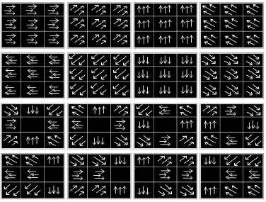
3.4. Optic Flow Data

The optic flow stimuli simulated the self-movement scene for 16 different heading

directions (Figure 21). The 16 directions were presented in a pseudo-random sequence until each

had been presented during 6-8 successful fixation trials. Each optic flow stimulus consisted of

500 white dots (0.19o at 2.61 cd/m2) on a black background (.18 cd/m2) stimulating the central

90o X 90o of the visual field. All dots were replaced by lifetime expiration (33 to 1000 ms) or by

a smoothing algorithm that maintained a uniform and consistent dot density across the stimulus

in all frames. Dots for these radial patterns accelerated as a sine X cosine function of their

distance from the focus-of-expansion maintaining an average speed of 40o/s.

Optic flow data was collected similarly to the singles data. The main difference is that

each flow stimuli displays motion from all nine segments of viewing area, emulating the

sensation of a specific self-motion. There are a total of 16 flow stimuli recording for each

35

Figure 22, flow stimuli, total 16 of them. Stimulus 1 through 16 is ordered from top left to

top right, then end as the lower right corner as the 16th stimulus. Each of those 16 flow

stimulus has most of the segments displaying motion. White arrows indicate the white dot’s

motion direction within that segment, where all 9 segments combined simulates self-motion

of the opposite direction from the dot’s motion. i.e. flow stimulus 9 has dots moving inward,

which simulates an backward self-motion to the viewing subject; flow stimulus 16 displays

36

15 1 1 1 1 1 1 1 1 1 1.154701 9.75 1.75 23 2 2 2 2 2 2 2 2 2 1

21.66667 3 3 3 3 3 3 3 3 3 3.282953 8 4 4 4 4 4 4 4 4 4 0 6 5 5 5 5 5 5 5 5 5 1.414214 22.5 6 6 6 6 6 6 6 6 6 1.5 27.75 7 7 7 7 7 7 7 7 7 3.326034 30.33333 8 8 8 8 8 8 8 8 8 2.333333 14.25 2 3 4 1 0 5 8 7 6 1.973787 14.75 6 7 8 5 0 1 4 3 2 1.931105 6 8 1 2 7 0 3 6 5 4 0.816497 17.33333 4 5 6 3 0 7 2 1 8 1.452966

4.5 6 6 7 5 5 0 4 4 3 0.5 20.75 2 2 3 1 1 0 8 8 7 1.887459

11.5 7 8 8 0 1 1 3 2 2 2.661453 10.6 3 4 4 0 5 5 7 6 6 1.122497

Figure 23, sample flow data from neuron 819R04. The flow data sheet follows the format

from the singles data, the apparent difference comes to almost fully-filled stimulus numbers

from column 2 through 10, which represents motion being displayed from segment 1 to 9

37

3.5. Doubles Data

The key of this thesis work is the collection and the analysis of the doubles data. The

doubles data are collected similarly as the singles data, except that during each testing, two

segments display motion simultaneously instead of just one. Since there are two segments

showing motion at the same time instead of one, we call it “doubles” data. To better organize the

testing of doubles testing pattern, a “hot spot” is selected from one of the nine segments. The hot

spot is a segment from one of the segments tested from a neuron's singles trial. Therefore, an X

neuron's hot spot could be segment 1, 3, 5, 7, or 9 (Figure 23); an O neuron's hot spot could be

segment 2, 4, 6, or 8; an XO neuron would have 2 hot spots: one from the X pattern and another

one from the O pattern segments. The hotspots are selected as the most excitatory spot from the

single’s recordings. The hot spots are also a reference spot, in which each hot spot is paired with

a “test spot” to form the doubles experiment. The test spot also must be one of the segments

tested from the neuron's singles run. Therefore, an X neuron's doubles experiment contains a

total of 64 entries of recording; an O neuron's doubles experiment contains a total of 52 entries of

recording; an XO neuron's doubles experiment may contain 116 entries since it contains a hot

38

Figure 24, doubles stimulus hot spot #1 first 16 stimulus. As the figure shows, each

“doubles” stimulus displays 2 segments of motion for recording. There is a “hotspot”

segment in which is always present, pairing with another spot we call it “test spot”. In this

case, the hotspot is the 7th segment, and since the 7th segment is a part of the X pattern, the

test spots are the 4 other segments that are part of the X pattern recording. This figure is

the first 16 double stimuli for an X neuron, where the hotspot is heading 0°. The next 16

stimuli would have the hotspot moving at 90° pairing with the test spots; then 180°, and

39

63.333 1 0 0 0 0 0 1 0 0 14.24 24.767 7.6 68 0 0 1 0 0 0 1 0 0 0

8.5 0 0 0 0 1 0 1 0 0 6.1305 99 0 0 0 0 0 0 1 0 1 8.7369 2.5 3 0 0 0 0 0 1 0 0 1.893 30.667 0 0 3 0 0 0 1 0 0 14.678

30.8 0 0 0 0 3 0 1 0 0 18.803 47 0 0 0 0 0 0 1 0 3 41 4.2 5 0 0 0 0 0 1 0 0 2.2891

1 0 0 5 0 0 0 1 0 0 0.57735 12.25 0 0 0 0 5 0 1 0 0 7.7715

1.5 0 0 0 0 0 0 1 0 5 1.5 22.333 7 0 0 0 0 0 1 0 0 7.4461

9 0 0 7 0 0 0 1 0 0 4.1473 164 0 0 0 0 7 0 1 0 0 5.5678 86.333 0 0 0 0 0 0 1 0 7 17.13

Figure 25, doubles sample data from neuron 819R10. Again, the data sheet follows the same

format as the singles and flow data sheet. This data is the recording of when hotspot is

moving towards 0°, as the 8th column (7th segment on screen) is showing the integer 1

through out the whole experiment, while pairing up with other X pattern segments moving

toward a planar direction. There are 4 test spots and 1 hotspot in a X neuron, and we test 4

planar motions per segment, therefore there are 16 entries for 1 planar motion of the

hotspot, making the total experiment having 64 entries from all 4 planar motion recordings

40

3.6. Interaction Effects in Doubles Recordings

It is commonly accepted in the field of neuroscience that local motion responses can be

“add up” to form the total flow response of a neuron, and that a neuron’s flow selectivity is

mostly consistent with its local motion selectivity summed up, which would suggest that the

separately collected singles data recordings would be fairly consistent with the neuron's flow

recordings if we puzzle together the appropriate combinations of the singles responses.

However, from the doubles hot spots recordings, we have noticed that at certain situations when

a combination of two segments are on, the resulting neuron firing rate can be as different as

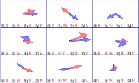
opposite of the neuron's singles data firing rate in the same segments. In one of the more clear

cases, neuron 819R10 seems to be displaying a reversal of selectivity effect triggered by the 7th

segment: 819R10’s singles has its X segments responsive when the motion on the screen is

moving to the left in general (Figure 25), however in the doubles recording, when the 7th

segment being the hotspot is showing rightward motion on screen, the neuron’s selectivity of

other x segments becomes reversed of its singles selectivity, they all becomes rightward

41

Figure 26, neuron 819R10 Single’s recording in terms of arrows. Each segment’s firing rate

responses from each planar motion is plotted; the length of each arrow indicates the

strength of the neuron’s response when that motion is displayed within that segment. The

strongest two responses are colored as red for easier viewing, which indicates mostly a

42

Figure 27, comparison of 819R10’s Singles X pattern arrow plot, 819R10’s Doubles X

pattern hotspot 180° plot, and 819R10’s Doubles X pattern hotspot 0° plot. The bottom 2

plots are the double’s plots when the hotspot (7th segment, having a red square) is showing

180° movement and its corresponding X patterned test spots, and when the hotspot is

showing 0° movement with its X patterned test spots. It is apparent that when the hotspot is

showing 180° movement, the test spot’s selectivity is more similar to that of its single’s

recording compared to when the hotspot is showing 0° movement: a clearly reversed

43

From the above firing rate illustrations, it is apparent that when specific combinations of

two segments are showing motion, the 2 segments interact and produces a drastically different

response comparing to just one of the 2 segments are being tested. The shift or the reversal of the

responses may also be a type of state-switching, where it is triggered by the hotspot’s motion

stimulus, in which it looks more like a template matching having the hotspot’s motion as its

reference. This finding explains why when puzzling together singles segmental responses to

predict flow responses is a flawed approach, since interaction requires more than one segment

that is displaying motion. The resulting responses from the doubles interaction also indicates that

a neuron's flow selectivity is much more complex than simply adding up local motion selectivity,

that it requires interaction effects to capture a better global selectivity of flow stimuli, resulting in

44

4. Methods

4.1. Training of the Dual Gaussian Model

The aim for the models is to see if singles and doubles model can predict their neuron’s

flow responses. We designed dual-Gaussian models of each MST neuron’s responses to the

singles and doubles local motion responses. Each neuron’s dual-Gaussian model is first trained

by fitting its singles data and then, in a separate step, trained by using its double data. Both

models are derived using the GA. All trainings are done in 3 separate trials of the GA, to provide

an index of the reliability of the model, particularly with respect to the avoidance of local

minima may obscure the actual global minimal error model.

4.1.1. Dual Gaussian Singles Models

The function of choice to model the MST neuron’s singles data firing rates is the Normal

Distribution function; also called the Gaussian function. It was chosen as a reasonable and

widely employed approximation to single neuron response directionality functions (Figure 27).

Dual models were used to accommodate the common impression that local motion mechanisms

include independent excitatory and inhibitory, or less often two excitatory or two inhibitory

mechanisms. The Gaussian function takes the following form:

2 2

-2

( , )

G

e

µ

σ

45

Figure 28, Gaussian curve, µ = 180, σ = 45. As employed in this modeling

effort, the ordinate represents normalized neuronal firing rate

and the abscissa represents local motion stimulus direction.

Since the data is pre-organized into nine different segments, we would need at least nine

Gaussian functions for each segment’s firing rate data. The Gaussian function represents the

preferred direction of motion for each segment. To visualize this, the x-axis of the Gaussian

curve represents the angle (direction) of the segment’s stimulus motion, with a range of 0 to 359

degrees and plotted to label the segment’s preferred direction as 180o from figure 27; the y-axis

represents the neuron’s firing rate when that stimulus direction is presented (Figure 27).

Therefore a Gaussian curve’s µ value represents the preferred direction for a specific segment’s

data, while σ value represents the selectivity of that segment’s firing rate responses. To take into

account potential excitatory and inhibitory responses in each response segment of a neuron’s

receptive field, we added a polarity indicator ( P ) for the Gaussian, which can be either +1 or -1

46

for each segment i, a gain constant ( C ) is applied to the Gaussian curve as well. The complete

function is therefore:

* (

,

) *

i i i i i

response

=

C

G

µ σ

P

We specified two Gaussians per segment to accommodate both excitatory and inhibitory

responses in a segment of the receptive field. In addition, the dual Gaussian models can fit the

bipolar (bi-directional) response functions observed in some segments. Finally, summing the

responses from all nine of dual Gaussian functions with the neuron’s singles baseline ( B )

creates a full accounting of the firing rate data in response to a local motion stimulus. These

baseline values were recorded during recording periods in which no motion stimulus is presented

on the screen, and is taken to be a good indicator of a neuron’s firing rate threshold between its

excitatory state and inhibitory state. Therefore, to obtain a response of a 9-segment singles dual

Gaussian receptive field models from any flow stimulus requires the following function:

4.1.2. Clamping

There is also a need to clamp any negative total response from the dual Gaussian model

47

responses are limited to firing at zero spikes per second, and there are no negative firing rates in

extracellular single neuron recordings. Therefore clamping negative total response to zero for

training the model captures this aspect of the recorded data. Our experience is that this clamping

yields better models.

4.2. Genetic Algorithm – Singles Model Training

After setting up the dual Gaussian functions for all 9 segments of the receptive field (total

of 18 Gaussians), each Gaussian’s parameters were tuned by the GA (genetic algorithm) to

produce the final summed response that match the singles or doubles data for that segment. To

obtain the proper values for each of the variables of the dual Gaussian functions for each

segment, the GA optimizes all of these variables.

4.2.1. Initialization

To initialize the modeling of each neuron, 2550 individual candidate dual Gaussian

models are randomly generated, with each individual Gaussian having the following variables to

be optimized: C, µ, σ, and P. Each candidate model also known as an individual of that

generation in the GA, is the 9-segment model that contains a dual Gaussian for each segment.

Therefore an individual contains 18 Gaussian functions with the above variables that will be

optimized throughout the GA process, and a fitness score indicating how well this individual is

preferred. C is initialized randomly to be between 0 and 200, µ is initialized randomly to be

48

between 0 to 15, with integer larger than 7 representing positive polarity, and negative otherwise.

4.2.2. Selection

For each neuron, each individual model’s fitness score is calculated, then the top 25

individuals are selected for the next phase. The fitness score function combines two different

aspects of each model’s fit to the neurophysiological data. The first fitness function calculates the

absolute error of an individual model’s firing rate responses to the neurophysiological responses.

The absolute error fitness function takes absolute value of the difference between the model’s

response and its corresponding single’s stimulus recorded response, then the difference is divided

by the standard error of this stimulus’ singles recording. This way, larger and smaller standard

error becomes meaningful in the training of the model.

20,16,36

1

model

data

absE

i

i

response

response

Fitness

standardError

=

−

=

∑

The second fitness function calculates the grouping error according to k-means clustering

algorithm. We apply a k-means clustering algorithm to the neurophysiological data assuming

three response clusters for each neuron that corresponds to classifying all responses as low,

medium, or high firing rates. In many cases, this clustering recognizes excitatory responses,

baseline firing responses, and inhibitory responses. Therefore, by having k-means clustering to

49

classified as group 1 (inhibitory group), 2 (baseline/no response group), and 3 (excitatory group).

(

, 3)

(

,3)

groupE model data

Fitness

=

∑

kMeans response

−

kMeans response

The fitness score for each model therefore includes calculated for both absolute error and

group error fitness scores. All of the individual models within the initial population are assessed

the same way to select 25 elite individual models from both fitness functions to make a total of

50

2 54 25 41 5 52 132 39 1 2 166 123 7 13 17 2 21 3 2 117 232 11 10 172 295 43 7 2 40 262 27 1 93 118 31 1 2 35 52 20 10 20 145 79 10 2 165 217 8 4 163 21 83 7 2 195 291 50 7 55 46 46 3 2 70 93 42 6 135 243 4 13 2 93 211 32 1 64 108 5 3

257.67 29 0 0 0 0 0 0 0

Figure 29, a randomly generated initial singles dual-Gaussian model (individual) by the GA

of neuron 712R02. Row 1 through 9 represents receptive field model’s 1st to 9th segment

selectivity dual Gaussians, 10th row represents the 2 fitness scores: absolute error is 257.67,

and group error is 29. Receptive field models all follow the same format as this example

comma separated data file. For row 1 to 9, the first column represents how many Gaussians

are in effect for that segment of the receptive field model; column 2 to 5 are the values for

the first Gaussian: column 2 is the Gain-Constant; column 3 is µ, means the tuning

direction preference; column 4 is σ, indicates how selective this Gaussian is; column 5 is the

polarity of this Gaussian – 8 or larger being positive and other wise negative polarity.

Columns 6 through 9 are the 2nd Gaussian’s parameters which all follows the same format

51

4.2.3. Crossover

Each individual model is consisted of genes, which are represented as binary bits. An

individual model’s genes are its variables that need to be optimized by the GA: C, µ, σ, and P.

The genes of an individual are crossed over with another individual (Figure 29), and the

individuals are provided from the Selection process. The 25 lowest absolute error individuals are

crossed over with the 25 lowest k-means grouping error individuals in the hope that their

crossed-over offspring will have both characteristics: better point to point matching and lower

variance. Each of the 25 lowest total error individuals are crossed over with each of the 25 lowest

grouping error individuals, and each parent produces four offspring. When crossing over from

the 2 parents, we are crossing over the parameters that correspond to each other: gain constant to

gain constant, µ to µ, σ to σ, and polarity to polarity from the 2 parents.

The four offspring from each parents are generated by randomly cutting from an index

point for each of the variables bit strings, split the variable bit string into two pieces from the

index point selected, then combine left piece from parent 1 first to right piece from parent 2 after,

right piece from parent 2 first to left piece from parent 1 after, left piece from parent 2 first to

right piece from parent 1 after, and right piece from parent 1 first to left piece of parent 2 after. If

any of the resulting crossed-over variables contains an invalid number that is larger than the

pre-set limit, such as 500 for µ, the value is then set back to the maximum number that value is

allowed, which is 359 in this case. After all 4 parameters of a Gaussian from each parents are

crossed over successfully, the 4 resulting parameters together represent the newly generated

offspring from the parents. The total offspring is 2500, adding the 50 elite parent individuals

52 individuals.

Figure 30, crossover of 2 parent’s gain constant.

4.2.4. Mutation

In case of any individuals that are locked in possible local minimum from the vast search

space, mutations of the genes are needed. The mutation factor is set as 0.05, and whenever a

random constant between 0 and 1 is less than 0.05, the mutation process will take place for any

candidate variable from an individual. For the variables that are to be mutated, a random index is

53

from 1 to 0 (Figure 30). Possible mutations are considered for every variable for all individuals.

Figure 31, example mutation of a given gain constant bit string. The randomly selected bit

is toggled.

The resulting population becomes the new generation, and is sent back into the selection

process for the loop. A singles dual Gaussian model is expected to take 75 generations of looping

in order to achieve a satisfactory result, whereas for doubles templates X and O would need just

35, due to less data and missing segment firing rates.

54

4.3. Genetic Algorithm - Doubles Model Training

Doubles dataset is different from the singles dataset, in which doubles experiment tests a

pair of segment instead of a single segment from the singles experiment. Therefore, this

difference requires some small modification of the GA training method, as well as how to utilize

the trained models in flow prediction.

4.3.1. Dual Gaussian Doubles Model and Template-Matching

Since the doubles data consists of responses to the selected hotspot paired with a test

spot, some adjustments are required for the GA to find a suitable dual Gaussian model. For each

doubles data file, the hotspot takes one of four planar directions, which is paired with all four

directions of the test spots of either the X or O configuration. In contrast to singles data in which

each segment evokes directional firing rates of its own, doubles data contains firing rates for a

pair of segments. For the GA to find a dual Gaussian model for the doubles data, we do not

assign any Gaussian or firing rate data to the hotspot, we only try to have GA find the

appropriate parameters for the test spot’s dual Gaussian, while using the paired firing rate as the

response to the test spot that the GA tries to fit.

The doubles data is fed into the GA to search for the optimized dual Gaussian curve for

each of the test spot’s segments. Note that for the hotspot, however, does not contain any

Gaussian functions, hotspot will only has identifiers indicating which direction it was tested. The

55

direction serves as a template, that when we use the doubles model to predict flow responses, we

use the doubles template in which the hotspot’s direction matches the flow stimulus’s direction at

hotspot’s segment (Figure 32).

There is a small difference between how doubles data is trained by the GA and that of the

singles: the singles models were trained by the GA optimizing all 9 segments’ dual Gaussian

together, while the doubles models were trained by the GA optimizing just a pair of hotspot and

test spot data at a time, then put back together into a full segments model. Besides the training

efficiency, there is technically no real difference between the two approaches of training as long

as the GA converges to a solution model over the generations. However, the doubles GA training

experienced difficulty in finding a good solution for some neurons, and by dividing the training

set into smaller data sets solved this problem. Therefore, the divide and conquer efficiency was

56

Figure 33, neuron 819R10’s doubles template for flow stimulus 1. This template is

constructed by finding the recording which has its hotspot direction matching the flow

stimulus that we are trying to predict, and for neuron 819R10, it has its X hotspot at the 7th

segment, and O hotspot at the 8th segment, therefore combining the X and O hotspot that

57

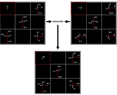
4.3.2. Doubles Diagonal Hotspot Data Interpolation

The singles data contains four planar direction’s firing rate responses for X, O, or both

patterns together. The doubles data was recorded the same way as singles. However, for

singles-to-flow prediction we just feed the singles model through the flow’s entire 16 stimuli. For the

doubles-to-flow prediction, we create templates for matching the segmental directions in each of

the optic flow stimuli. The problem with this is that flow was recorded with diagonal motions,

whereas neither singles nor doubles were recorded with any diagonal motion, singles and

doubles were only recorded with the 4 planar motions. Therefore, in order to construct diagonal

hotspot motion templates, we interpolate for the double’s diagonal hotspot motion’s test spot

firing rates from the data we have.

The doubles data was recorded by presenting just one of the four planar direction motion

stimuli for a hotspot segment paired with a test spot segment. To interpolate for a neuron’s

doubles data X pattern hotspot 45° and X test spot firing rates, simply take the average of hotspot

0° firing rates and 90° firing rates for every tested segment. Repeat the same steps through all of

the other diagonal motion of the hotspot for doubles until all of the diagonal hotspot and test spot