This is a repository copy of
Synthesizing Real-Time Schedulability Tests using
Evolutionary Algorithms : A Proof of Concept
.
White Rose Research Online URL for this paper:
http://eprints.whiterose.ac.uk/152205/
Version: Accepted Version
Proceedings Paper:
Dziurzanski, Piotr orcid.org/0000-0001-9542-652X, Davis, Robert Ian
orcid.org/0000-0002-5772-0928 and Soares Indrusiak, Leandro
orcid.org/0000-0002-9938-2920 (Accepted: 2019) Synthesizing Real-Time Schedulability
Tests using Evolutionary Algorithms : A Proof of Concept. In: Proceedings of the 40th IEEE
Real-Time Systems Symposium. . (In Press)
[email protected] https://eprints.whiterose.ac.uk/
Reuse
Items deposited in White Rose Research Online are protected by copyright, with all rights reserved unless indicated otherwise. They may be downloaded and/or printed for private study, or other acts as permitted by national copyright laws. The publisher or other rights holders may allow further reproduction and re-use of the full text version. This is indicated by the licence information on the White Rose Research Online record for the item.
Takedown
If you consider content in White Rose Research Online to be in breach of UK law, please notify us by
Synthesizing Real-Time Schedulability Tests using
Evolutionary Algorithms: A Proof of Concept
Piotr Dziurzanski
Department of Computer Science University of York, York, UK
Robert I. Davis
Department of Computer Science University of York, York, UK
Leandro Soares Indrusiak
Department of Computer Science University of York, York, UK
Abstract—This paper assesses the potential for mechanised assistance in the formulation of schedulability tests. The novel idea is to use evolutionary algorithms to semi-automate the process of deriving response time analysis equations. The proof of concept presented in this paper focuses on the synthesis of mathematical expressions for the schedulability analysis of messages on Controller Area Network (CAN). This problem is of particular interest, since the original analysis developed in the early 1990s was later found to be flawed. Further, as well as known exact tests that have been formally proven, there are a number of useful sufficient tests of pseudo-polynomial complexity and closed-form polynomial-time upper bounds on response times that provide useful comparisons.
Index Terms—real-time systems, schedulability analysis, evo-lutionary algorithms, Controller Area Network
I. INTRODUCTION
Real-time systems are characterised by the need for both functional and timing correctness. Verifying the timing cor-rectness of a real-time system is typically framed as a two step process:timing analysisseeks to characterise the amount of time that each task can take to execute, or each message can take to be transmitted. Using this information, schedula-bility analysis aims to characterise the worst-case end-to-end response time of functionality involving one or more tasks or messages, taking into account the way in which they are scheduled and any interference between them. An upper bound on the worst-case response time can then be compared to the deadline to determine if timing requirements can be met.
It is interesting to consider how schedulability tests are typically devised. Usually this is a creative manual process. Researchers try to determine the worst-case possible sce-nario(s) given a model of the behaviour of the system, its tasks, messages, and scheduling policies. Often these worst-case scenarios are derived via pencil-and-paper or white-board examination of how the system may behave, with schedules depicted for a small number of tasks or messages. In some cases, theorems and proofs are derived proving prop-erties of the worst-case scenario(s). From a consideration of these worst-case scenarios, researchers then look to construct schedulability tests or response time analyses that upper bound the response times for any valid scenario. Thus providing some form of guarantee that each task or message will always meet its deadline, provided of course that the system behaves as modelled, and the assumed worst-case scenario really does
represent the worst-case. Informal proofs of the correctness of schedulability tests are often made via hand-crafted logical arguments checked by co-authors and reviewed by peers. Further efforts at validation are usually done via simulation. While simulation of large numbers of synthetically generated task or message sets cannot prove correctness, since not every scenario can be considered, they can sometimes show that an analysis technique is flawed (i.e. optimistic) by revealing a counter-example. Such corner-cases can be very rare, and may not always be revealed by this form of verification.
The research literature on real-time scheduling is littered with the bodies of flawed proofs of theorems that appeared to the authors, peer reviewers, and many readers to be correct when first published, but were later found to be incorrect. High profile examples include the original analysis for Controller Area Network (CAN) published by Tindell et al. [33]–[35] in 1994-5 that was subsequently shown to be incorrect by Bril et al. [7] in 2006 and comprehensively refuted, revisited, and revised by Davis et al. [11] in 2007. (Interestingly, Di Natale and Zeng [22] showed that this flaw is exposed by only around one-in-a-million synthetically generated message sets). More recently, in 2015, Nelissen et al. [23] discovered flaws in scheduling theory for self-suspending tasks [18] published in 2010, with a subsequent critical review by Chen et al. [9] in 2018 felling a whole swathe of subsequent research in this area. Another example is the early analysis of wormhole routing on a Network-on-Chip (NoC) by Shi and Burns [32] published in 2008. This analysis was shown to be optimistic by Xiong et al. [39] in 2016. They presented a revised analysis, only for that method to be proven optimistic by Indrusiak et al. [14] later that same year. In response to these problems, recent efforts at mechanised formal proofs for real-time analysis [8] are beginning to gain traction, with recent work on the PROSA project1 aiming to formally prove the revised CAN schedulability analysis [11].
In this paper we address a related aspect of the overall prob-lem of schedulability analysis. System models are gradually improving in their fidelity and thus taking into account more detailed behaviours; however, this is making both worst-case scenarios and sound response time equations more difficult to derive. The main contribution of this paper is to propose
mechanised assistance to researchers in the formulation of schedulability tests. Specifically, we propose the use of evo-lutionary algorithms to semi-automate the process of deriving response time analysis equations. While the research effort on PROSA seeks to provide a means ofproof-assistancefor use in real-time scheduling problems, we aim to complement that by providing a means of formulation-assistance.
Utilising the proposed semi-automated formulation assis-tance, the overall work flow for a particular scheduling prob-lem can be summarised as follows. First, researchers consider the system model and scheduling policies used, and determine a set ofsymbolsandoperatorsforming agrammarthat can be used to express response time analysis equations that could po-tentially provide solutions to the problem. Second, they obtain a set ofverification vectors. Each verification vector represents a concrete system, and provides the parameter values for all of the entities that are scheduled in that system, as well as their indicativeresponse times. The indicative response times are guaranteed lower bounds on the worst-case response time, and are typically obtained via measurements taken from: (i) a real system, (ii) a cycle-accurate simulation of the system, or (iii) a simulation using an appropriate high level model. The grammar and the verification vectors are used as inputs into the formulation assistant. The formulation assistant uses an evolutionary algorithm to create populationsof candidate
response time equations that comply with the grammar. Each candidate equation is evaluated against the data for every entity in the set of verification vectors, resulting in a set of
computedresponse times. Thefitnessof the candidate equation is then determined by comparing the set of computed response times that it produces with the set indicative response times. High fitness implies that the computed response times provide a tight upper bound on the indicative response times. The evolutionary algorithm creates subsequentgenerationsof can-didate equations by recombining and mutating cancan-didates from the previous generation that are selected with a probability depending on their fitness. This selection pressure ensures that the overall fitness of the population increases over a number of generations, and the algorithm is able to find individual candidates with high fitness. The best candidate equations are returned as the output of the formulation assistant.
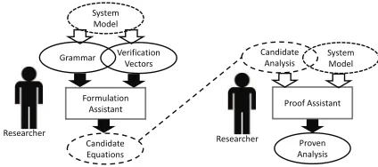
The aim of using a formulation assistant to provide sugges-tions for response time equasugges-tions is not to supplant researchers in this area, but rather to help them in finding effective response time analyses that can be explored in more detail, including being subject to both informal and formal proof, which remains the responsibility of the researcher. The overall processes is illustrated in Figure 1, which depicts researchers taking a system model and using it to create a grammar and a set of verification vectors that form the inputs to the formulation assistant. The formulation assistant produces candidate equations that can be checked and refined by the researcher. In a final step, the resulting candidate analysis may be checked via a proof assistant to provide the final proven schedulability analysis.
One of the benefits of using an evolutionary approach to
Candidate Analysis
Formulation
Assistant Proof Assistant
Researcher
Grammar Verification Vectors System Model
Candidate Equations
Proven Analysis Researcher
[image:3.595.327.539.45.139.2]System Model
Fig. 1. Overall process of deriving proven analysis.
assist researchers in this way is that it can potentially find a range of equations from simple yet effective tests that may be useful for fast design space exploration, to more complex tests that provide more precise results. The approach is flexible and can potentially be seeded with equations that are known to be correct for simplified versions of the problem, enabling exploration of a family of similar scheduling problems. Fur-ther, it removes the need for researchers to implement multiple different candidate schedulability tests, since each one is tested automatically against the verification vectors.
This use of verification vectors is both a potential pitfall and an advantage. If there are corner cases and worst-case scenarios that are not captured in the set of verification vectors, then there is clearly the potentially for the equations produced to be optimistic, as indeed is the case with an entirely manual process. However, whenever such corner cases are found they can simply be added to the set of verification vectors and the process re-run to find better solutions that correctly account for those scenarios. As future work, not explored in this paper, we also envisage the co-evolution of verification vectors along with the candidate equations.
In the real-time domain, evolutionary algorithms have pre-viously been applied on a variety of problems including:
(i) Task mapping and allocation for distributed [24], [20] and Network-on-Chip [19], [27]–[30] systems;
(ii) Test data generation aimed at finding worst-case execu-tion times [36]–[38], [2]; and
(iii) Stress-testing reactive real-time systems with the aim of finding task arrival patterns that result in missed deadlines [5], [6].
Although employing evolutionary techniques, all of these works differ from the research reported in this paper in terms of both the type of problem addressed and the type of evolutionary methods used. To the best of our knowledge, the research reported here represents the first application of evolutionary techniques (specifically genetic programming / grammatical evolution) to the problem of finding schedulabil-ity tests for real-time systems. (A preliminary publication of our concept and ideas appeared in arXiv [15]).
II. BACKGROUND
In this section, we provide a brief background on Symbolic Regression, Genetic Programming, and Grammatical Evolu-tion.
Symbolic Regression is a form of regression analysis that searches the space of mathematical expressions to find a formula that best fits the measurement data provided. As a simple example of symbolic regression, one might try to determine the mathematical expression or formula for the remaining area A of an ellipse which has a semi-minor axis of length x, a semi-major axis of length y, and a circular area removed from it of radius x, based on the following data set (x, y, A): (1,1,0), (1,2,3.14), (1,3,6.28), (1,4,9.42), (2,2,0), (2,3,6.28), (2,4,12.57). Note, the correct formula is (xy −x2)π. While symbolic regression has long been
the province of mathematicians, during the 1990s effective computerized approaches were developed based on Genetic Programming [17] and Grammatical Evolution [25], [26].
Genetic Programmingintroduced by Koza [17] in the early 1990s is based on the concept of an evolutionary algorithm which operates on a population of candidate computer pro-grams. Each candidate program is represented by a tree structure, i.e. a graph with nodes, edges, and terminals (leaves), where the nodes are functions (for example +, −, ∗, /,
min, max) and the terminals are symbols (for example x,
y, 1, π). By contrast genetic algorithms typically represent candidate solutions via fixed-length coded strings of numbers. With Genetic Programming the population is first initialised with a randomly generated set of candidate programs, with tree structures occupied by combinations of the available functions and symbols. The fitness of each candidate program is then evaluated by executing it using the input values from the measurement data provided, and comparing the resulting output to the reference value associated with those inputs. The smaller the deviation from the reference value the greater the fitness. Subsequent generations of candidate programs are created via evolution by recombining and mutating candidate
programs from the previous generation that are selected on the basis of their fitness. This selection pressure acts to improve the overall fitness of the population over the generations. Hence, after a number of generations the method is typi-cally able to find candidate programs with high fitness. Re-combination involves selecting a node at random on each of two candidates and then swapping the sub-trees at that point. Mutation, on the other hand, selects a node or a terminal at random and replaces it with a randomly selected function or symbol. Alternatively, a randomly selected sub-tree may be replaced by another randomly generated sub-sub-tree. For example, using prefix notation, two possible candidates aimed at computing the remaining area A of the ellipse mentioned earlier are: (∗ π (− (∗ y y) (∗ x x))) and (∗ π (+ (∗ x y) (∗ y y))). Via re-combining, the next generation might include (∗ π (+ (∗ x y) (∗ x x))) with further mutation giving (∗ π (− (∗ x y) (∗ x x))), which is in fact the correct solution. For an introduction to the main principles of Genetic Programming, including detailed illustrative examples, see the work of Sette and Boullart [31].
Grammatical Evolution introduced by Ryan and O’Neill [25], [26] in the late 1990s retains the fundamental concepts of Genetic Programming; however, rather than performing the evolutionary process on the actual programs, Grammatical Evolution represents candidate programs as expressions in the form of variable length strings encoded according to a gram-mar defined in Backus–Naur Form (BNF). These strings are then evolved via re-combination and mutation operations that respect the specific rules of the defined grammar. Grammatical Evolution has the advantage that the rules of the grammar provide direct control over precisely how the functions and symbols may be combined. It permits implementation in any programming language, and produces solutions that can be translated into an arbitrary programming language or simply interpreted as mathematical expressions.
For the proof-of-concept formulation assistant described in this paper, we make use of an approach based on Grammatical Evolution. We selected an evolutionary approach in preference to Tabu Search or Simulated Annealing because the mutation and crossover operators can easily be applied over grammar trees, and the population-based approach supports parallelism. Further, with Grammatical Evolution the grammar rules pro-vide control over how functions and symbols are combined which is useful in applying domain knowledge to the problem.
III. CONTROLLERAREANETWORK
message will win arbitration and continue to send its message. The other nodes will cease transmitting and wait for the bus to become idle again before attempting to re-transmit their messages. (Full details of the CAN physical layer protocol are given in [3]). In effect CAN messages are sent according to fixed priority non-pre-emptive scheduling.
A. Background Research on CAN
In 1994-5, Tindell et al. [33]–[35] showed how research into fixed priority scheduling for single processor systems could be applied to the scheduling of messages on CAN. The analysis of Tindell et al. provides a method of calculating the maximum queuing delay and hence the worst-case response time of each message on the network. In 2007, Davis et al. [11] corrected significant flaws in this early analysis that could potentially result in it providing guarantees for messages that could subse-quently miss their deadlines during operation. As with all fixed priority systems, appropriate priority assignment is essential to achieve schedulability at high bus utilisations. Davis et al. [11] also showed that Deadline minus Jitter Monotonic Priority Order, claimed by Tindell et al. to be optimal for CAN, is not optimal with respect to exact schedulability tests; and that Audsleys Optimal Priority Assignment (OPA) algorithm [1] is required in this case. Subsequently, Davis and Burns [10] introduced the concept of robust priority ordering, able to best tolerate additional interference due to errors on the bus.
B. System Model
In this section we describe the system model and nota-tion used to analyse the worst-case response times of CAN messages. The system is assumed to consist of a number of nodes connected to each other via a CAN bus. Each node is assumed to ensure that whenever arbitration starts on the bus, the highest priority message queued at that node is entered into arbitration. A fixed set of hard real-time messages are transmitted over the network. Each message i has a unique priority and is transmitted by a single node. We overload i
to mean either message ior priority ias appropriate. We use
hp(i)to denote the set of messages with priorities higher than
i, andlp(i)to denote those with priorities lower thani. Each messageihas a maximum transmission time ofCi. The event
that triggers queuing of an instance of message i is assumed to occur with a minimum inter-arrival time of Ti, referred to
as the message period. Each message i has a hard deadline
Di, corresponding to the maximum time allowed from the
initiating event for an instance of the message to the end of its transmission, at which point the message data is available on the receiving nodes that require it. The deadline of each message is constrained to be less than or equal to its period (Di≤Ti). Each messageiis assumed to be placed in a queue
and available for transmission in a bounded time Ji after its
initiating event, where Ji is the release jitter of the message.
The worst-case response time Ri of message i is defined as
the maximum possible delay from the initiating event for an instance of that message, until it is received at the receiving nodes. A message is schedulable if its worst-case response
time is less than or equal to its deadline (Ri≤Di). A system
is schedulable if all of its messages are schedulable.
C. Existing Schedulability Analysis
In this section we recapitulate the exact and sufficient schedulability analysis for CAN given by Davis et al. [11]. The worst-case response time of messageican be determined by examining the response time of all instances of message
i that occur within a priority level-i busy period; assuming that message i and all higher priority messages are released with their maximum jitter at the start of the busy period, and then subsequently re-released as soon as possible. Further, immediately before the initial release of these messages, the longest message of lower priority than ibegins transmission.
Biis the blocking factor at priorityi, equivalent to the longest
transmission time of any message of lower priority:
Bi= max
k∈lp(i)(Ck) (1)
In the following, we use the index variable q to represent an instance of message i. The first instance, released at the start of the busy period corresponds to q = 0. The longest time from the start of the busy period to instanceqbeginning transmission is given by the solution to the following fixed point equation:
wim+1(q) =Bi+qCi+
k∈hp(i)
wm
i (q) +Jk+τbit
Tk
Ck (2)
Note τbit is the time for one bit to be transmitted on the
bus. The summation term represents interference from higher priority messages that can win arbitration over message i
and so delay its transmission. Iteration starts with a value of w0
i(q) = Bi + qCi, and ends on convergence when
wni+1(q) =wni(q), or whenJi+wni+1(q)−qTi+Ci> Di in
which case the message is unschedulable. The response time of instanceqis given by:
Ri(q) =Ji+wi(q)−qTi+Ci (3)
and the worst-case response time of messageiis given by:
Ri= max q=0...Qi−1
(Ri(q)) (4)
where Qi is the number of instances of message i in the
priority level-i busy period (see [11] for details of how Qi
is computed). For ease of reference, we refer to the exact schedulability test given by (2), (3), and (4) asE1.
As shown by Davis et al. [11], when messages have con-strained deadlines, an upper bound on the worst-case response time of messageimay be found by computing the maximum queuing delay wi using the following fixed point iteration,
where the revised blocking term max(Bi, Ci) accounts for push-through blocking from previous instances of the same message:
wni+1=max(Bi, Ci) +
k∈hp(i)
wn
i +Jk+τbit
Tk
Here, iteration starts with a suitable initial value such asw0
i =
max(Bi, Ci), and ends whenwin+1+Ji+Ci> Di in which
case the message is unschedulable, or when wni+1 = wn i in
which case the message is schedulable and an upper bound on its worst-case response time is given by:
Ri =Ji+wi+Ci (6)
This sufficient test is used in commercial schedulability anal-ysis tools, for example Mentor Graphics Volcano Network Architect toolset2, due to its ease of implementation, speed of operation, and extensibility [12].
D. Simplifying the Schedulability Tests
Below, we re-arrange the sufficient test given by (5) and (6) removing the queuing delay wi which is in effect a working
variable. Since we measure time in units ofτbit, this value can
be replaced by 1. Further, since∀k Ck> τbitthen⌈(x+1)/y⌉
can be replaced by⌊x/y⌋+1to give an equivalent formulation. We refer to this sufficient test asS1.
Ri=Ji+Ci+max(Bi, Ci)+
k∈hp(i)
Ri−Ji−Ci+Jk
Tk
+ 1
Ck (7)
We note that due to the fixed point iteration required to find a solution, this equation has pseudo-polynomial time complex-ity. It can be simplified to give a closed-form polynomial time over-approximation by substitutingDiforRion the right hand
side. Thus we have sufficient test S2:
Ri=Ji+Ci+max(Bi, Ci)+
k∈hp(i)
D
i−Ji−Ci+Jk
Tk
+ 1
Ck (8)
Further simplifications are possible, retaining sufficiency at the cost of a further degradation in precision. For example, since
−Ji−Ci within the floor function can only reduce the value
obtained this can be removed, hence we have sufficient test
S3:
Ri=Ji+Ci+max(Bi, Ci) +
k∈hp(i)
D
i+Jk
Tk
+ 1
Ck
(9) Finally, the original flawed schedulability test of Tindell et al. [33]–[35] can be expressed as follows. We refer to this test as F1:
Ri=Ji+Ci+Bi+
k∈hp(i)
Ri−Ji−Ci+Jk
Tk
+ 1
Ck
(10) Note the close similarity betweenS1andF1, which differ only in the blocking term, withBi substituted for max(Bi, Ci).
We use schedulability tests S1, S2, S3, F1, and the exact testE1 as a basis for comparisons in Section V.
2http://www.mentor.com/products/vnd/communication-management/vna/
IV. FORMULATION-ASSISTANT
In this section, we describe the generic framework used to implement a formulation assistant aimed at helping re-searchers to find effective schedulability tests for real-time systems, in the form of response time analysis equations.
The idea of a formulation assistant starts from an underlying assumption that for a system composed ofn entities that are scheduled, a sound upper bound on the worst-case response time of each entity i can be formulated as an equation in the canonical form: Ri = <expr>, where <expr> is a
complex expression composed, via an appropriate grammar, from further nested expressions, operators, and terminals
comprisingsymbolsrepresenting the parameters of the system. The set of available symbols and operators must be defined by the researcher, with due consideration for the schedul-ing problem at hand, and the dimensionality of the results produced (see Section IV-B). The symbols and operators provide the fundamental building blocks from which appro-priate response time analysis equations can be constructed. Symbols can include various parameters (Xi) of entityi, such
as its period (Ti) and deadline (Di), and parameters of the
system itself, such as the number of processors. Operators can include simple arithmetic functions with two arguments such as addition, subtraction, max, and min, as well as compound operators made up of multiplication, ceiling, and floor. More complex operators are also possible including summation that iterates over sub-sets of entities, with an additional index variable k permitting the use of further symbols (e.g. Xk)
pertaining to each of these. Further, recursive equations are possible, since the symbolRi may also appear in expressions
on the right hand side of the equation (see Section IV-D for details of how these are evaluated). Finally, since response times are measured in integer units of processor or network clock cycles, we assume that all values used are integers, and all operators use integers as their input and output values.
We note that when designing a grammar, it is essential that the set of operators fulfil the closure property, meaning that each operator is able to process all possible values generated by other operators and the symbols (i.e parameters). Further, the grammar must also besufficient in the sense that it must be possible to solve the problem using the proposed set of op-erators and symbols [31]. As well as an appropriate grammar, the method relies on a set ofverification vectors. Each vector provides theparameter valuesfor all of the scheduled entities in a concrete system, as well as theirindicativeresponse times. The indicative response times are guaranteed lower bounds on the worst-case response time of that entity, and may be obtained via measurements taken from: (i) a real system, (ii) a cycle-accurate simulation of the system, or (iii) a simulation using an appropriate high level model.
population of candidate equations at random and evaluates theirfitness. The fitness of a candidate equation determines the probability that it will be selected to produce new candidates in the nextgenerationvia recombination with other candidates and mutation. The idea is that this selection pressure ensures that the overall fitness of the population increases over a num-ber of generations, and the algorithm is able to find individual candidate equations with high fitness, i.e. good solutions to the optimisation problem considered. The objective or fitness function is key to this.
The fitness of each candidate equation is determined with respect to the set of verification vectors. Each candidate equation is evaluated for each entity in each verification vector, using the parameter values stored in the vector. This results in a computed response time. The computed response times are compared to the indicative response times to determine the overall fitness of the candidate equation.
A. Fitness Function
The fitness function compares the indicative response times from the verification vectors with the computed response times produced by a candidate equation. The design of the fitness function is vitally important in finding good quality solutions to the optimisation problem considered.
For a given candidate equation, fitness is computed for each of the n entities in each of the V verification vectors. The overall fitness is then simply the sum of these nV fitness values. For each entity, the pair of indicative Rindic
i and
computedRcompi response times are compared, and the fitness
function defined as follows:
F =
⎧
⎪ ⎪ ⎨
⎪ ⎪ ⎩
0 Rcompi =Rindic
i
min100,Rcompi
Rindic
i −1
Rcompi > Rindici
W1−Rcompi
Rindic i
Rcompi < Rindici
(11)
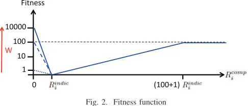
If the computed response time is equal to its indicative counterpart, then the equation provides perfect analysis, and the contribution to the fitness function is zero. Alternatively, if the computed response time is greater than its indicative counterpart, then the candidate equation at least provides a sound analysis, even though it may not be a good one. In this case, the fitness depends on the degree of over-approximation up to a limit (a 100-fold over-approximation). Finally, if the computed response time is smaller than its indicative counterpart, then the equation does not provide sound analysis. In this case, the fitness depends on both the degree of under-approximation, and the weighting factor (W > 1) used to penalise unsound results. Here, the largest value that can be obtained is F = W, which occurs when the computed response time is zero.
As the evolutionary algorithm iterates over a number of generations, the weighting factor W used in the fitness function is varied to adjust the amount of tolerance given to unsound equations. Initially, W = 1 giving a balance between under and over-approximation. Assuming there are
G generations in total, then W is increased exponentially
Fitness
W
0 (100+1)
10000
[image:7.595.314.557.44.148.2]1 100 10
Fig. 2. Fitness function
for the first G/2 generations up to W = 10000, meaning that a single under-approximation (Rcompi = 0) contributes a
fitness score equal to having a two-fold (Rcompi = 2Rindici )
over-approximation for 10,000 entities. (More precisely, for generationg= 0. . . G/2,W = 10000(2g/G)). For the second G/2 generations, W = 10000 permitting the algorithm to refine the resulting expressions against an unchanging fitness function. Figure 2 illustrates how the fitness function varies with the value of Rcompi and the weighting factor used to penalise under-approximation ofRindic
i .
Note that although the fitness function was derived ac-cording to the arguments given above, and refined via the evaluation of different variants (see Section VI), a systematic study of the most appropriate fitness functions to use remains an avenue for future work.
B. Dimensionality and Scale-Invariance
It is important that the grammar is designed to ensure that the expressions generated have the correctdimensionality, i.e. produce values in the same units as the response timeRi.
This ensures that the candidate equations produced are also
scale-invariant, meaning that it does not matter what scale the unit of measurement has, provided that it is used consistently throughout. These properties can be achieved by ensuring that all of the operators produce outputs that are of the same type and dimensionality as their inputs.
Since parameters such as the period Ti, deadline Di and
response time Ri are measured in the same units of time,
expressions such as Ri =Di are dimensionally correct. By
contrast, an expression such asRi=Di∗Diis dimensionally
incorrect, since the right hand side evaluates to a quantity that is in units of time squared. Assigning such a value to
Ri would be both incorrect and meaningless. The operators
add, subtract, min, max, and summation all result in the same units (dimensionality) for their outputs as their inputs, whereas multiply and divide (including floor and ceiling) do not. To preserve the correct dimensionality of the resulting expression, every multiply operation has to be exactly matched by a corresponding divide (either floor or ceiling) and vice-versa. To ensure that this is the case in our proof-of-concept imple-mentation we make use of compound operators, effectively
C. Grammar Operators and Symbols
In this subsection, we outline the grammar used to describe response time equations. The basic grammar given below is appropriate for problems of fixed priority preemptive or non-preemptive scheduling on a single processor or network. The set of operators fulfil the essential closure property, meaning that each operator is able to process all possible values generated by other operators and the terminal symbols (i.e parameters). The canonical form of the candidate equations is: Ri =<expr>, where <expr> is expressed in Backus–
Naur Form in the text box at the end of this sub-section. Note in this grammar, we use the symbols*and$, and*
and /to represent multiply combined with ceiling, and mul-tiply combined with floor as follows: C*(A$B) = ⌈A/B⌉C,
C*(A/B)=⌊A/B⌋C. Further,˜and_are used to represent the max and min operators, thus (A˜B) = max(A, B) and (A_B) = min(A, B). Finally, the sigma operator evaluates the summation of its second operand over the set of values specified by its first operand(<range>), which can indicate values ofkfrom the setslp(i),lep(i),hp(i),hep(i), andall(i) i.e. all priorities.
The grammar is designed to constrain the complexity of the expressions that can be produced in a number of ways. Firstly, sigma (i.e. summation) terms are not per-mitted to nest inside other summations. This is enforced by
<exprInSum> which does not includesigma expressions. Similarly, the compound operators for multiply combined with ceiling and multiply combined with floor are not permitted to nest inside floor or ceiling expressions. This is enforced by <exprInFloorCeil>. The grammar further enforces that parameters indexed byk, the iterator in summations, are only permitted within summations. This is enforced via the use of <kVar> and<kNumDenVar>. Further, the response time can only be composed of multiples of the parameters representing blocking Bi, release jitter Ji, transmission time
(or execution time)Ci, and interferenceCk. Other parameters
such as Ti, Tk, and Jk can only contribute to the values of
the multipliers. This is enforced via the separation between
<iVar> and <iNumDenVar>, and between <kVar> and
<kNumDenVar>.
For experiments seeking to find non-recursive expressions, the grammar permits the use of the deadlineDias a proxy for
the response time on the right hand side of the expressions. In the grammar for recursive expressions this is simply replaced by Ri in the definition of <iNumDenVar>. Note that the
deadlines of other entities (e.g. Dk) have no impact on the
response time, since deadlines are in effect arbitrary points in time, that do not affect the actual schedule produced. Hence
Dk does not appear in the grammar.
With the exception of deadlines, explained above, all of the message parameters from the system model used for the analysis of CAN (see section III) are included in the grammar. Note, the blocking factor Bi is also included even though it
is a simple compound term. This is done because formulation assistance requires domain knowledge, and it is reasonable to
assume that researchers would know that blocking is important in any form of fixed priority scheduling.
Note that although many of the CAN schedulability analysis equations, for example (7) to (10) include the term “+1” in addition to a floor function, we do not permit the constant1in the grammar. This is because the constant1is a dimensionless quantity, and its use would prevent expressions from being dimensionally correct and scale-invariant. Instead, we note that the addition of the denominator to the numerator in a floor or ceiling function is the same as “+1”, i.e. ⌊(A+B)/B⌋ =
⌊A/B⌋+ 1 hence use of the constant1 or indeed any other value that is not derived from the set of parameters is not essential in the derivation of correct equations.
<test> ::= Ri = <expr> <expr>::=
(<expr><op><expr>)|<iVar>|
<expr>*(<exprInFloorCeil>$<exprInFloorCeil>)| <expr>*(<exprInFloorCeil>/<exprInFloorCeil>)| sigma(<range>)(<exprInSum>)|((<expr>)˜(<expr>))| ((<expr>)_(<expr>))
<exprInSum>::=
(<exprInSum><op><exprInSum>)|<iVar>|<kVar>|
<exprInSum>*(<exprInSumFloorCeil>$<exprInSumFloorCeil>)| <exprInSum>*(<exprInSumFloorCeil>/<exprInSumFloorCeil>)| ((<exprInSum>)˜(<exprInSum>))|
((<exprInSum>)_(<exprInSum>)) <exprInFloorCeil>::=
(<exprInFloorCeil><op><exprInFloorCeil>)|<iVar>| <iNumDenVar>|sigma(<range>)(<exprInSumFloorCeil>)| ((<exprInFloorCeil>)˜(<exprInFloorCeil>))| ((<exprInFloorCeil>)_(<exprInFloorCeil>)) <exprInSumFloorCeil>::=
(<exprInSumFloorCeil><op><exprInSumFloorCeil>)| <iVar>|<kVar>|<iNumDenVar>|<kNumDenVar>| ((<exprInSumFloorCeil>)˜(<exprInSumFloorCeil>))| ((<exprInSumFloorCeil>)_(<exprInSumFloorCeil>))
<op>::=+|-<range>::=forall_k_InLp_i|forall_k_InLep_i|forall_k_InHp_i| forall_k_InHep_i|forall_k
<iVar>::=Bi|Ci|Ji <kVar>::=Ck
<iNumDenVar>::=Ti|Di (or in the recursive case ::=Ti|Ri) <kNumDenVar>::=Tk|Jk
D. Recursive Equations
Since candidate equations may include the symbol Ri on
the right hand side (RHS) they are assumed to be potentially recursive and therefore to require iterative evaluation. Iterative evaluation starts using an initial value, equivalent to the response time without any interference (i.e. Ji+Ci) for any
Ri symbols on the RHS of the equation. The equation is then
evaluated, producing a new value for Ri. This value is then
substituted for anyRisymbols on the RHS ready for the next
iteration, and so on. The intermediate results of evaluating the equation are monitored on each iteration, and a number of rules and constraints are applied to ensure viable behaviour. These rules are designed to permit the evolution of equations that converge towards a solution in either a monotonic or non-monotonic way (for example, similar to the behaviour of a binary search). The rules are as follows: (i) If the result is the same on two consecutive iterations, then it has converged and iteration is terminated. All equations without Ri on the RHS
defined by the researcher. We note that a reasonable limit is required in practice to avoid excessive run times. A limit of 100 iterations is used in our proof-of-concept experiments. (iii) If a negative value, divide by zero, or too large an integer is produced, then iteration is terminated. In the case of a negative value, the result is assumed to be zero, which is a very poor value from the perspective of the fitness function. In the case of a divide by zero, or too large an integer, the final result is assumed to be the largest integer represented by the implementation. Again, this is also a poor value from the perspective of the fitness function.
V. PROOF-OF-CONCEPTEVALUATION
In this section, we describe evaluation of the proof-of-concept formulation assistant on the problem of CAN schedu-lability analysis. Here, we aim to evolve simple but effective analysis formulated as a single expression that is directly comparable to existing schedulability tests S1, S2, S3, and
F1for CAN. We note that the exact testE1is more complex, requiring a two stage process. Evolving such tests is beyond the scope of this initial investigation.
A. Verification Vectors
The verification vectors for the proof-of-concept implemen-tation were obtained assuming a CAN bus using 11-bit mes-sage identifiers. First, we randomly generated 100 verification vectors of 20 messages each as follows: The periodTiof each
message was chosen at random according to a log-uniform distribution from the range 5 to 500ms; thus generating an equal number of messages in each time band (e.g. 5 to 50ms, 50 to 500 ms etc.). The deadline of each message was chosen at random according to a uniform distribution in the range 0.5Ti to Ti. Thus all messages had constrained deadlines,
with a minimum deadline of 2.5ms, and a maximum deadline of 500ms. The release jitter of each message was chosen at random according to a uniform distribution in the range 0 to 0.5Di. The number of data bytes was chosen at random
according to a uniform distribution in the range 1 to 8 bytes. The priorities of the messages were assigned in Deadline minus Jitter (Di−Ji) monotonic priority order.
The timing characteristics of each verification vector (mes-sage set) were adjusted to obtain the desired total network utilisation. This was done by scaling the period, deadline, and release jitter of every message by the same factor. Five message sets were thus obtained for each of the 20 utilisation levels from 50% to 97.5% in steps of 2.5%. (This equates to a variety of bus speeds in the range 66KBits/sec to 250KBits/sec).
In addition, a further 25 verification vectors were generated (5 for each of the 5 utilisation levels from 25% to 35% in steps of 2.5%) using the same parameters as described above, but with their priorities assigned at random. (See section VI for a discussion as to why we added these vectors).
Finally, we also generated 10 verification vectors that high-light the flaw in the original analysis of CAN. These message sets were deemed schedulable by the schedulability testF1, but
are in factunschedulableaccording to the exact testE1. Due to the difficulty in generating such message sets, each comprised 10 messages, with 8 data bytes, implicit deadlines (Di=Ti),
zero release jitter, and utilisation levels from 95% to 99.5%. Priorities were assigned in Deadline Monotonic order. The 10 message sets revealing this flaw were found from a total of approx. 100,000 message sets with these characteristics.
In experiments 1-3 we determined the indicative response times (Rindic
i ) using exact analysis. This gives the evolutionary
algorithm the best possible data to work from3. We then relaxed the quality of this data in experiment 4 to see if the evolutionary algorithm could still produce high quality candi-date equations from imperfect data, similar to that produced via simulation or measurement in cases where the worst-case scenario(s) are unknown. Note, we did not use simulation to generate indicative response times, since to do so would raise the question of what to simulate. As the worst-case scenario is known for CAN, simulation of that scenario would only serve to provide a slow means of finding the exact worst-case response times. Instead we used the analytical form of exact analysis, as that provides a ground truth to compare against, and can be evaluated quickly. We then controlled the degree of approximation of the indicative response times fed into the evolutionary algorithm, as described in the following section. Note that since all message sets considered in our proof-of-concept evaluation had a total utilisation of strictly less than 1, we were able to use exact analysis to calculate the exact response time for each message irrespective of whether it was schedulable or not. This was achieved by only terminating the fixed point iteration in (2) on convergence, rather than when the deadline was exceeded.
B. Parameter Settings for the Grammatical Evolution
We used the EpochX open source genetic programming framework (v1.4.1) to implement Grammatical Evolution. The basic parameter settings used were as follows: population size 1000, number of generations 2000, mutation rate 0.1 (with mutation of a small number of symbols permitted at the same time). The form of selection used was Fitness Proportionate Selection, where the probability of selecting each candidate for re-combination is determined in proportion to the reciprocal4 of it fitness value. We repeated each experiment 500 times, recording the single best result from each run. We then took the 50 top results from this set (see Section VI for a discussion as to why we did this). The verification vectors used contained 100 message sets in Deadline minus Jitter monotonic priority order, of which 43 were schedulable; 25 message sets in random priority order, of which 7 were schedulable, and 10 message sets that reveal the flaw in test F1, none of which were schedulable. The parameters of the message sets were as described in Section V-A.
3This is representative of problems where exact response times can be
found by simulating over the hyperperiod, but efficient schedulability tests are unknown.
4The reciprocal of the fitness value is used, since in our experiments smaller
C. Results
To assess the quality of the results produced, we made use of a larger set of assessment vectors that were not used in the evolutionary process. These were generated in the same way as the verification vectors, but contained 10 times as many message sets. The assessment vectors contained 1000 message sets with priorities in Deadline minus Jitter monotonic priority order, of which 421 were schedulable; 250 message sets in random priority order, of which 48 were schedulable, and 100 message sets that highlighted the flaw in test F1, none of which were schedulable. Note, the fitness values referred to in the remainder of the paper are with respect to the assessment vectors (i.e. Assessment Fitness).
Test Assessment Fitness Num. of optimisticRcomp
i
S1 1702 0
S2 12038 3
S3 16445 0
F1 244889 100
E1 0 0
Ri= 0 260000000 26000
Ri=Di 3681912 5038
TABLE I
[image:10.595.326.565.46.91.2]ASSESSMENT FITNESS OF EXISTING SCHEDULABILITY TESTS
Table I gives the fitness values for the existing schedulability tests, including the sufficient tests:S1,S2, andS3, the flawed test F1, and the exact testE1. Also shown is the fitness for
Ri= 0andRi=Di. Note that the exact testE1has a fitness
of zero, as it provides perfect results. The flawed testF1has a fitness score of 1501, slightly better than that of testS1(1582), if the assessment vectors that expose the flaw are omitted; however, adding those vectors increases its fitness score to 244889 due to 100 optimistic values of Rcompi . Note, testS2
also results in 3 optimistic values for Rcompi , this may seem surprising since the test is sufficient; however, the optimistic values occur for cases where the message is unschedulable (Rindic
i > R comp
i > Di) and is correctly identified as such by
the test. AssumingRi= 0results in the maximum (i.e. worst
possible) fitness score of 260000000, since the response time of every one of the 2600 messages in the assessment vectors is underestimated by the maximum amount. Assuming that
Ri=Dialso results in poor fitness due to the fitness function
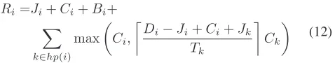
heavily penalising the unschedulable cases (Rindic i > Di). 1) Experiment 1: Baseline: As a baseline, we used the formulation assistant with no recursion permitted (i.e. Ri
excluded from the grammar), precise indicative response times acting as a ground truth, and none of the corner cases that expose the flaw in test F1. The best candidate expression that was found is shown below, and then repeated after simplification as an equation. The fitness of this equation is 12624, which is comparable to the fitness (12038) of test S2
that also does not includeRi in its formulation. This equation
did not result in underestimation of response times for any messages in the assessment vectors.
((Ji+sigma_(forall_k_InHp_i)
(((Ci)˜(Ck*(((Tk+(Ci+(Jk-(Ji-Di))))-Tk)$Tk)))))+(Bi+Ci))
Ri=Ji+Ci+Bi+
k∈hp(i) max
Ci,
D
i−Ji+Ci+Jk
Tk
Ck
(12)
The mean fitness of the top 50 results in this experiment was 21651 and the mean number of optimisticRcompi values
was 8.84, with 7 expressions producing no optimistic values, and 9 others producing 3 or fewer optimistic values, similar to testS2.
2) Experiment 2: Adding Recursion: Here, we added the possibility of recursion to the baseline settings by includingRi
instead of Di in the grammar. The best candidate expression
that was found is shown below, and then repeated after simplification as an equation. The fitness of this equation is 3084, which is a substantial improvement over the fitness (12038) of test S2, while still some way from the fitness (1702) of testS1that also includesRi in its formulation. This
equation did not result in underestimation of response times for any messages in the assessment vectors.
((((Ji+(Bi+(Ci+sigma_(forall_k_InHp_i)(Ck)))))˜(Bi)) +sigma_(forall_k_InHp_i)(Ck*(((Ri-(Ji-Jk))
-((((Tk)˜(Ck)))˜(((Jk)˜((Bi+((Tk-Ji)-Ck)))))))$Tk)))
Ri=Ji+Ci+Bi+
k∈hp(i)
R
i−Ji+Jk−max(0, Bi−Ji−Ck)
Tk
Ck
(13) The mean fitness of the top 50 results in this experiment was 27918 and the mean number of optimisticRcompi values was 8.98, with 13 expressions producing no optimistic values. Note, it would appear that the small amount of pessimism in both (12) and (13) is enough to avoid / obscure incorrect classification of the corner cases, even though these equations were generated without regard to them.
3) Experiment 3: Adding Corner Cases: Here, we added extra verification vectors that reveal the flaw in testF1. Again, recursion was permitted, and precise indicative response times provided a ground truth. The best candidate expression that was found is shown below, and then repeated after simplifica-tion as an equasimplifica-tion. The fitness of this equasimplifica-tion is 3096, which is very similar to the fitness (3084) of the best expression from experiment 2, while still some way from the fitness (1702) of testS1that also includesRi in its formulation. This equation
did not result in underestimation of response times for any messages in the assessment vectors.
(Bi+(Ci+(Ji+sigma_(forall_k_InHp_i)
(Ck*((((((((Ri)_(Tk)))˜(Ck)))_(Jk))+(Ri-Ji))$Tk)))))
Ri=Ji+Ci+Bi+
k∈hp(i)
R
i−Ji+ min(max(Ri, Ck), Jk)
Tk
Ck (14)
The mean fitness of the top 50 results in this experiment was 20816 and the mean number of optimistic Rcompi was
4) Experiment 4: Adding Approximation: This experiment was the same as experiment 3, except that we approximated the indicative response times with respect to the ground truth. Approximate indicative response times used values chosen at random from a uniform distribution in the range [0.8Rexact
i , Rexacti ]. Note, in the case of unschedulable
mes-sages (with Rexact
i > Di), this could potentially cause them
to appear to be schedulable.
The best candidate expression that was found is shown below, and then repeated after simplification as an equation. The fitness of this equation is 4710, which is worse that the fitness of the best expressions from experiments 2 and 3 (3084 and 3096), but still considerably better than the fitness of the polynomial time testsS2andS3. Again, this equation did not result in underestimation of response times for any messages in the assessment vectors.
((Ji+(Bi+Ci))+sigma_(forall_k_InHp_i) (Ck*((((Ci+Ri)+Jk)-Ji)$Tk)))
Ri =Ji+Ci+Bi+
k∈hp(i)
R
i−Ji+Ci+Jk
Tk
Ck (15)
The mean fitness of the top 50 results in this experiment was 27575 and the mean number of optimistic Rcompi was 29.02, with only 6 expressions producing no optimistic values. This degradation in performance with respect to experiment 3 is due to the use of less precise indicative response times.
It is interesting to note that there is substantial common-ality in the resulting expressions from experiments 1–4. In particular, certain building blocks often occur, for example
Ji+Ci+Biand the summation overhp(i)withCk multiplied
by some factor in the numerator and Tk in the denominator.
Further, Ri,+Jk, and−Ji often appeared in this multiplier.
These building blocks are present in the known sufficient tests. (Note ⌈XY+1⌉=⌊XY⌋+ 1 when X and Y are positive integers, thus floor and ceiling operators can be interchanged in approximate formulae where all parameters are positive integers).
5) Experiment 5: Random Search: Finally, we note that a purely random search is ineffective at generating useful formulae. Repeating experiment 3 for 50 runs with purely random generation of 2,000,000 expressions that comply with the grammar resulted in a best expression with a fitness of 56477, compared to a best of 3096 for the evolutionary algo-rithm. The best expression found via random search is shown below, and then repeated after simplification as an equation. We note that in common with other expressions found by random search, this equation returns values no smaller than the message period, which is an easy but inaccurate way of avoiding underestimating the response time in the majority of cases, but also deems almost every message unschedulable, since all messages have constrained deadlines (Di≤Ti).
(((((((((((Ji)˜(Bi)))˜(Bi*(Ci$Ri))))˜(Ci*(Ti$Ci))))˜(Ji)))˜ (Ji))+sigma_(forall_k_InHp_i)(Ck))
Ri=
Ti
Ci
Ci+
k∈hp(i)
Ck (16)
VI. LESSONSLEARNED
In this section we discuss the lessons learned in developing a proof-of-concept formulation assistant that can be used to derive expressions for response time analysis of CAN messages. During development we made improvements in four main areas:
1.Improving the grammar:
a) Dimensionality: We restricted the use of ceiling, floor, and multiply to only appear as compound operations. This ensured that all expressions produced were scale invariant and dimensionally correct, and therefore meaningful. b) Nesting restrictions: We constrained the use of the
sum-mation operator preventing it from being nested within another summation, since this led to expressions that were very complex and slow to evaluate. Similarly, we prevented ceiling and floor functions from nesting within other ceiling or floor functions.
c) Symbol restrictions: We noted that due to the way in which the system is scheduled, the actual response times can only be composed of multiples ofCi,Bi,Ji, andCj. We
therefore restricted the other symbols such as Ti, Tj, Jj
to only appear within the multipliers for expressions that included those former symbols.
2.Improving the Verification Vectors:
a) Correlations between parameters: Correlations between parameter values had to be avoided, as this can lead to the inappropriate substitution of one parameter for another. The initial verification vectors we used had all of the messages in Deadline minus Jitter monotonic priority order. This resulted in strong correlations between the value of
Di and the values of Dj for higher priority messages,
and similarly between Ti and Tj. As a consequence,
the evolutionary algorithm would often find high fitness, but flawed expressions that contained summations of the deadlines or periods of higher priority messages. This issue was addressed by including additional vectors with random priority ordering.
b) Range of values for variables: The verification vectors used required careful consideration to ensure sufficient variability in parameter values. This was necessary, because the evolutionary approach cannot distinguish between pa-rameters that always take the same or very similar values. Initially, release jitter was set to a small range of values from 0 to 2.5ms. We found that this resulted inJi or Jj
appearing in the evolved expressions as a proxy for Ci
or Bi, hence producing flawed equations. This problem
was addressed by expanding the range of jitter values. For similar reasons, we ensured that the message lengths were variable (1-8 data bytes), rather than a fixed size, and therefore that Ci, Cj, and Bi could be distinguished. We
also used constrained deadlines so thatTi andDi, andTk
3. Tuning the Grammatical Evolution:
a) Fitness Function: As with any evolutionary algorithm, the design of the fitness function is vitally important. In particular, the form of the fitness function needed to heavily penalise under-approximation of indicative response times; however, applying a heavy penalty to the early generations of candidate equations can be counter-productive, hence the variable weighting factor W used in our implementation. We experimented with different values for W. We found that improved results were obtained if we increased the value of W over the first half of the generations up to a value of 10,000. We tried values ofW =1, 10, 100, 1,000, 104,105, and 106, with notable improvements up to 104,
but not thereafter. We therefore used W = 10,000. b) Offset to the Fitness Function: We explored adding an
offset of 0, 0.5, 1, 2, 4, and 8 to the value returned by the fitness function for each message. This offset impacts the fitness proportionate selection, with larger offsets giving a higher probability that weaker candidates would still be included in the selection. We found no significant improvement using non-zero offsets and hence used zero. c) Number of Generations: We explored the effect that the
number of generations: 500, 1000, 2000, 5000, had on the performance of the evolutionary algorithm. We found that increasing the number of generations beyond 2000 had no significant effect on the quality of the resulting expressions. We therefore used 2000.
d) Escaping from local minima: Search based on Grammatical Evolution is a trade off between exploration of the vast search space andexploitation, i.e. searching in the vicinity of good solutions. Small changes to an expression can easily result in large changes in computed response times and hence fitness, which causes difficulties in escaping from evolutionary dead-ends (local minima). To mitigate this problem, we repeated each experiment 500 times, taking the results of the best 50 runs.
4. Improving the implementation:
a) Parser implementation: The standard EpochX parser is capable of handling arbitrary expressions (i.e. Java code) and as a consequence is relatively slow when all that is needed is to parse simple mathematical expressions. We implemented our own parser, which amounts to approxi-mately two pages of Java code, this improved the overall run time of the evolutionary algorithm by a factor of approximately 100.
b) Parallel execution: We used a high performance compute cluster to evolve the 500 populations for each experiment in parallel. This resulted in an overall elapsed time for each experiment of approximately 48 hours.
VII. CONCLUSIONS
In this paper, we introduced the idea of a formulation assistant to aid researchers seeking to derive schedulability tests for real-time systems. Our proof-of-concept formulation assistant focused on the problem of deriving schedulability analysis equations for Controller Area Network (CAN) using Grammatical Evolution of expressions.
The main contributions of this work are as follows: (i) We showed that an approach based on Grammatical
Evolution is viable and can provide interesting insights into the schedulability analysis equations required. (ii) The best equations produced by the formulation assistant
were broadly similar in quality to known sufficient schedulability tests, when measured against a large set of assessment vectors.
(iii) The equations produced were viable and showed a rel-atively small degradation in quality when approximate rather than exact response times were used as the basis of the fitness function. This indicates that the approach could be effective when the input data is derived from simulation, i.e. in cases where exact response times are unknown.
(iv) The lessons learned in the development of the proof-of-concept formulation assistant, discussed in Section VI. There are a number of interesting directions for future work. These include:
• An Island-based approach: We intend to explore an
island-based approach that enables the re-combination and evolution of the best solutions found from a number of different island populations that are first evolved in parallel and then combined. The aim being to avoid the algorithm becoming trapped in evolutionary dead-ends (local minima).
• Unsolved schedulability analysis problems: We intend to
apply the formulation assistant concept to both solved and unsolved schedulability analysis problems, particular in the area of Network-on-Chip, using simulation as a means of determining indicative response times.
• Co-evolution of verification vectors: Since simulation
can typically only provide necessary schedulability in-formation as reference data, it is important to try and avoid candidate equations being wrongly classified as
sufficient, when in fact in some cases they can under-estimate the exact response times. We therefore intend to explore the co-evolution of the verification vectors alongside the population of candidate equations. The aim being to identify corner cases, improving the quality of the verification vectors and hence also the resulting schedulability analysis expressions.
We note that the schedulability analysis equations derived by the formulation assistant approach are ultimately only as good as the verification and assessment vectors used. While we expect that the vectors themselves can be improved via co-evolution, there is still no guarantee that all relevant corner cases will be discovered. This is where the approach links back to researchers with experience in schedulability analysis who can interpret the expressions derived, simplify them and seek to prove their correctness by other means, such as employing proof assistance.
experiments 1 – 4 provide sufficientschedulability tests. The sketch proofs showing that (12) and (15) provide sufficient tests and the counterexamples showing that (13) and (14) do not, illustrate the way in which formulation assistance is intended to be used by researchers. Formulation assistance provides a means of finding candidate schedulability analysis equations, but does not fully automate the process of deriving schedulability tests. The burden of proof that such tests are sufficient remains with the researchers. They can interpret, refine, and simplify the expressions found via formulation assistance, develop proofs (possibly employing automated proof assistance) and also construct counter examples, which can in turn be used to refine and improve the verification and assessment vectors used by the evolutionary algorithm.
APPENDIX
In this appendix, we examine whether the best expressions returned by the evolutionary algorithm in experiments 1 – 4 provide sufficientschedulability tests.
To show that the expression with the best fitness from Experiment 4, i.e. (15) provides a sufficient test, we make use of the proven exact schedulability analysis for CAN [11]. This analysis needs to examine all instances of messagei that are released within a priority level-ibusy period. The lengthLi of
this busy period is given by Eq. (8) in [11]. IfLi≤Ti−Jithen
this busy period ends before the release of the next instance of messageiand hence only the first instance of that message need be examined to determine schedulability. Equivalently, if the solutionL∗
i to the following fixed point iteration, starting
from an initial value of L∗
i = Ji+Ci, does not exceed Ti,
then only the first instance of message ineed be examined to determine schedulability. (Note, that when L∗
i ≤Ti only one
instance of messageioccurs within the busy period and so its contributionCi is taken outside of the summation).
L∗
i =Ji+Ci+Bi+
k∈hp(i)
L∗
i −Ji+Jk
Tk
Ck (17)
Re-writing and simplifying the exact test i.e. (2) and (3) for the case where q = 0, schedulability of the first instance of message i can be checked via the following fixed point iteration, starting from an initial value of R∗
i =Ji+Ci.
R∗
i =Ji+Ci+Bi+
k∈hp(i)
R∗
i −Ji−Ci+Jk+τbit
Tk
Ck
(18) Together, (17) and (18) form a sufficient schedulability test. If L∗
i ≤ Ti, then only the first instance of message i need
be checked to determine schedulability, and ifR∗
i ≤Di, then
that first instance is schedulable.
To prove that the best expression from Experiment 4 (15) provides a sufficient test, we need only show that if Ri ≤
Di in (15), then it follows that both L∗i ≤ Ti in (17) and
R∗
i ≤ Di in (18). Comparing (15) and (17) the two fixed
point iterations are identical except for the extra +Ci term in
the numerator of the ceiling function in (15). Since Ci >0,
it follows that L∗
i ≤Ri (as computed by (15)) and hence if
Ri ≤ Di, we have L∗i ≤ Ri ≤ Di ≤ Ti. Comparing (15)
and (18) the two fixed point iterations are identical except that the +Ci term in the numerator of the ceiling function
in (15) is replaced by +τbit−Ci in (18). Since Ci > 0 >
τbit −Ci, it follows that R∗i ≤ Ri (as computed by (15))
and hence if Ri ≤ Di, we have R∗i ≤ Ri ≤ Di. Thus if
messagei is deemed schedulable according to (15) then it is also schedulable according to the sufficient test comprising (17) and (18), hence (15) also provides a sufficient test.
Using the above result, we can also show that the best expression from Experiment 1, i.e. (12) also provides a suf-ficient test. Comparing (12) and (15), we can ignore the Ci
term inside themax()function in (12) as this term can only make the computed value ofRifrom this equation larger. The
only remaining difference between (12) and (15) is then the substitution ofDi for Ri within the numerator of the ceiling
function. It follows that whenever (12) computes a value for
Ri ≤Di, then the value computed by (15) can be no larger,
and thus also indicates schedulability. Since (15) provides a sufficient test, so does (12).
Next, we show that the expression with the best fitness from Experiment 3, i.e. (14) does not provide a sufficient test. This can be seen from the following counter example with three messages. The message parameters (Ci, Di, Ti,
Ji, Bi) measured in bit transmission times are as follows:
message 1 (125, 1000, 1000, 750, 125), message 2 (125, 375, 10,000, 0, 125), and message 3 (125, 10,000, 10,000, 0, 0). Equation (14) computes the response time of message 2 as 375; however, the exact value is 500. This occurs when message 1 exhibits its maximum release jitter of 750 and is released simultaneously with message 2, just as message 3 starts transmission. Message 1 is then released again 250 bit times later leading to a sequence of transmitted instances of messages 3,1,1,2, and a response time of 500 for message 2. Message 2 is therefore unschedulable, and hence (14) which deems this message schedulable doesnot provide a sufficient test. (We note that this counterexample points to the need for improved verification and assessment vectors that permit large values for release jitter, creatingback-to-back interference).
Finally, we show that the expression with the best fitness from Experiment 2, i.e. (13) also doesnotprovide a sufficient test. This can be seen from the following counterexample with three messages as follows: message 1 (65, 200, 200, 0, 135), message 2 (65, 10,000, 10,000, 0, 135), and message 3 (135, 10,000, 10,000, 0, 0). Equation (13) computes the response time of message 2 as 265; however, the exact value is 330. This occurs when messages 1 and 2 are released simultaneously, just as message 3 starts transmission. Message 1 is then released again 200 bit times later leading to a sequence of transmitted instances of messages 3,1,1,2, and a response time of 330 for message 2. The reason that (13) does not provide a sufficient test can also be seen via comparison with (18), which is an exact test when the priority level-i busy period includes only one instance of message i, as is the case here for message 2. Since (18) is exact, yet (13) can result in a smaller computed value ofRi when Bi−Ck > Ci−τbit, it