A Machine Learning Approach to Predicting Coverage in Random Wireless Networks

This is a repository copy of

A Machine Learning Approach to Predicting Coverage in

Random Wireless Networks

.

White Rose Research Online URL for this paper:

http://eprints.whiterose.ac.uk/136499/

Version: Accepted Version

Proceedings Paper:

El Hammouti, H, Ghogho, M and Zaidi, SAR (2019) A Machine Learning Approach to

Predicting Coverage in Random Wireless Networks. In: Proceedings of 2018 IEEE

Globecom Workshops (GC Wkshps). 2018 IEEE Globecom Workshops (GC Wkshps),

09-13 Dec 2018, Abu Dhabi, United Arab Emirates. IEEE . ISBN 978-1-5386-4920-6

https://doi.org/10.1109/GLOCOMW.2018.8644199

© 2018 IEEE. This is an author produced version of a paper published in Proceedings of

2018 IEEE Globecom Workshops (GC Wkshps). Personal use of this material is permitted.

Permission from IEEE must be obtained for all other uses, in any current or future media,

including reprinting/republishing this material for advertising or promotional purposes,

creating new collective works, for resale or redistribution to servers or lists, or reuse of any

copyrighted component of this work in other works. Uploaded in accordance with the

publisher's self-archiving policy.

eprints@whiterose.ac.uk https://eprints.whiterose.ac.uk/

Reuse

Items deposited in White Rose Research Online are protected by copyright, with all rights reserved unless indicated otherwise. They may be downloaded and/or printed for private study, or other acts as permitted by national copyright laws. The publisher or other rights holders may allow further reproduction and re-use of the full text version. This is indicated by the licence information on the White Rose Research Online record for the item.

Takedown

If you consider content in White Rose Research Online to be in breach of UK law, please notify us by

A Machine Learning Approach to Predicting

Coverage in Random Wireless Networks

Hajar El Hammouti

, Mounir Ghogho

and Syed Ali Raza Zaidi

∗_{International University of Rabat, FIL, TICLab, Morocco}

†_{University of Leeds, School of EEE, UK}

{hajar.elhammouti,mounir.ghogho}@uir.ac.ma,s.a.zaidi@leeds.ac.uk.

Abstract—There is a rich literature on the prediction of coverage in random wireless networks using stochas-tic geometry. Though valuable, the existing stochasstochas-tic geometry-based analytical expressions for coverage are only valid for a restricted set of oversimplified network scenarios. Deriving such expressions for more general and more realistic network scenarios has so far been proven intractable. In this work, we adopt a data-driven approach to derive a model that can predict the coverage probability in any random wireless network. We first show that the coverage probability can be accurately approximated by a parametrized sigmoid-like function. Then, by building large simulation-based datasets, the relationship between the wireless network parameters and the parameters of the sigmoid-like function is modeled using a neural network.

Index Terms—Coverage probability, sigmoid function, neural networks, machine learning, stochastic geometry.

I. INTRODUCTION

Motivated by its tractability, researchers have widely adopted stochastic geometry to model wireless net-works performance and understand their behaviors [1]. Valuable and insightful stochastic geometry-based ana-lytical expressions can be found in the literature [2– 7]. However, to ensure tractability, these expressions are based on many simplifying assumptions on the wireless network, which are often unrealistic [2]. For general network setups, deriving analytical expressions to predict performance is very often unfeasible.

The following three scenarios illustrate the above-mentioned limitations.

• Correlated shadowing: most stochastic geometry-based studies have either neglected shadowing in the channel modeling, or assumed it to be a spa-tially independent process, following a log-normal distribution. Indeed, when spatial correlation is considered, tractability of the analytical derivations is in general no longer possible with stochastic geometry theoretical tools. The authors in [8], [9] have considered correlated shadowing but assumed a particular shadowing model and ignored the path loss component to make the derivations tractable. Another approach that has been proposed in the literature is to approximate the interference, which includes a large number of log-normally distributed

shadowing terms, by a gamma distribution which simplifies the derivations of the coverage probabil-ity; see for example [10].

• Non-homogeneous base station distribution: most stochastic geometry-based studies model the po-sitions of the base stations using a homogeneous Poisson point process (HPPP). While this simpli-fies the analysis, it does not capture the repulsive nature of the spatial topology observed in real-world cellular networks; several works have shown that base stations locations are better modeled us-ing a Mat´ern hard-core point process (HCPP) [5], [11]. This more realistic modeling however under-mines the tractability of the analytical analysis of network performance [12].

• Deterministic base station deployment: deriving a closed-form expression for the average coverage probability in this scenarion is a challenging task. Indeed, random spatial distribution models for BS positions simplify the analytical derivations. In-troducing specific locations of BS in the network generally undermines the tractability of the deriva-tions [6].

The main objective of this paper is to propose an easy-to-apply and practical approach to predicting net-work performance for any given netnet-work setup, which is characterized here by several network features describ-ing the channel modeldescrib-ing, the base station distribution, user association scheme, etc. Our approach is data-driven and borrows machine learning tools to determine an accurate mapping between the network features and its performance. In this paper, the performance metric is the coverage probability of a typical user, but the approach could be applied to other performance metrics.

A. Related work

Even with such assumptions, advanced mathematical techniques are involved in order to compute the cov-erage probability. As reported in [4], five techniques are commonly used to calculate coverage probability in stochastic geometry based networks. In general these techniques either (i) rely on the Rayleigh fading as-sumption, (ii) consider only the dominant or a limited number of the nearest interferers, (iii) approximate the probability density function (pdf) of the sum of the interference, (iv) use Plancherel-Parseval theorem, (v) or finally, invert the moment of the generating function to obtain the pdf of the interference. These many complicated mathematical processes involved in cover-age probability computation make it difficult to have an easy-to-apply and practical approach to coverage prediction. Under these circumstances, the development of a general framework that captures the real complexity of the network system and proposes accurate, yet simple and direct, coverage probability prediction is of a great importance.

In the last few years, there has been a large interest in machine learning (ML) techniques to provide accurate analytical models based on the statistical analysis of data [13]. The main success of machine learning tech-niques can be attributed to its ability to map various network parameters to the network’s response. Unlike the theoretical tools provided by stochastic geometry, a ML based approach captures the real complexity of the network by running a large number of measurements and/or experiments and proposes a mapping between input features and the output feature (network perfor-mance).

In [14] and [15], comprehensive surveys on the potential use of machine learning in 5G networks and wireless sensor networks, respectively, are provided. In [16], the authors compare a measurements-based pre-diction model to the signal-to-interference-and-noise-ratio (SINR) theoretical model. The paper shows that the ML approach outperforms the traditional SINR based model by providing results that are closer to the real measurements. Their ML approach is also used to predict the achievable throughput, and can thus be used for resource allocation optimization. In [17], the authors describe the experimental environment and methodologies to model the throughput of a trans-mission control protocol connection. The experimental results therein show that the throughput can be predicted with a very high accuracy using a support vector machine model [18]. In [19], the authors show that operators and service providers can adapt their services and contents using prediction models based on user’s experience feedback. In particular, a supervised ML technique is proposed to overcome video starvation in large-scale wireless networks. Other machine learning applications can be found in [20] and [21]. In [20],

a machine learning approach is proposed for drones to build a radio map that supports their path planning and positioning. In [21], the authors propose a neural network based approach for a better handover decision in heterogeneous networks. This approach was shown to improve the quality of service perceived by the users. In [22], the authors propose a distributed deep neural network to learn the optimal power allocation for a device-to-device network. The main advantage of such an approach is to reduce the computational complexity caused by optimization-based algorithms.

B. Contribution

In this work, we are interested in the prediction of coverage probability of a typical user in a random wireless network using machine learning. To the best of our knowledge, this has not been addressed before. The contribution of this paper is twofold.

1) First, by running a large number of simulations, we show that the coverage probability can be closely approximated using a parametrized sigmoid-like function.

2) Second, we propose to use the exceptional ability of neural networks (NN) to approximate compli-cated functions in order to estimate the parameters of the sigmoid-like function from the feature set that characterizes the random wireless network, namely: base stations spatial intensity, path loss ex-ponent, Nakagami-channel parameter, log-normal shadowing variance, log-normal spatial correlation, the BS transmit power, and background noise variance. This modeling is carried out for two user-association schemes.

C. Structure

The rest of the paper is organized as follows. The next section describes the studied system model. Section III presents the proposed coverage probability approxima-tion. Section IV proposes a method to learn the model’s parameters using NN, and presents accuracy results. Finally, concluding remarks and possible extensions of this work are provided.

II. SYSTEMMODEL

-3000 -2000 -1000 0 1000 2000 3000 x

-3000 -2000 -1000 0 1000 2000 3000

y

Typical user Base station

(a)

-3000 -2000 -1000 0 1000 2000 3000

x -3000

-2000 -1000 0 1000 2000 3000

y

Typical user Base station Guard zone radius

(b)

-1500 -1000 -500 0 500 1000 1500

x -2000

-1500 -1000 -500 0 500 1000 1500 2000

y

Typical user Base station position Hexagonal pattern

(c)

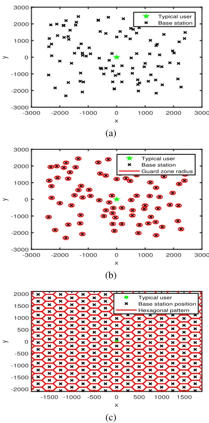
Fig. 1: (a) A PPP realization of base stations withλ= 4.4∗10−6_BS/m2_{, (b)}

A HCPP realization of base stations extracted from a PPP withλ= 4.4∗10−6

BS/m2

whenRc = 200m, (c)256BS positions following a hexagonal

pattern.

schemes: (i) the user is associated with the nearest base station (Nearest Base station Association Scheme, NBAS), (ii) the user is served by the BS that provides the best signal-to-interference-and-noise ratio (SINR) (SINR Maximization Association Scheme, SMAS). Let b0denote the BS serving the typical user. In this paper,

we focus on the downlink communication. The SINR experienced by the typical user is given by

SINR = d

−α

b0 Gb0gb0Pb0

σ2₊ P

b6=b0

d−_bαGbgbPb

, (1)

where Pb is the transmit power of BS b, db is the distance between the typical user and BSb,α∈[2,6]is the path loss exponent,Gbis the channel power gain due to shadowing, gb is the small-scale fading power gain.

In our simulations, we focus on the following setup: all BS transmit powers are equal to each other i.e. Pb = Pb0 =P, ∀b; the small-scale fading follows the general

Nakagami distribution, i.e. gb ∼ Γ(m,_mω) follows a gamma law of parameters (m, ω

m); the shadowing is log-normally distributed, i.e.log(Gb)∼ N(0, σ2s). and is spatially correlated; the spatial correlation between two shadowing gains depends on the distance between the corresponding BS, as described by 3GPP in [23], i.e. the correlation between the shadowing gains associated with BS i and BS j, R(i, j), is an exponentially decreasing function of the distance separating the two BS,∆di,j, and soR(i, j) =exp(−∆_dcordi,j)where dcor is

the correlation distance which controls the strength of the spatial correlation.

We are interested in the coverage probability of the typical user, which is defined as the probability that the SINR of that user is above a given thresholdτ, i.e.

pc(τ) =P(SINR> τ). (2)

In the case of hexagonal grid model for BS positions, we assume that the center of the grid is random in order to be able to use the same definition for the coverage probability as in the case of PPP and HCPP models.

III. MODELING THE COVERAGE PROBABILITY We have generated a large number of network setups with different values of the path loss exponent, BS intensity, Nakagami channel parameter, transmit power-to-noise ratio γ = P/σ2_{, variance of shadowing and}

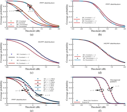
correlation distance, and for each network setup, we have generated a large number of network realizations. For each network setup, we have estimated the average coverage probability for typical values of the threshold τ. Examples of these estimation results are provided in Fig. 2. For each network setup, curve-fitting using the non-linear least squares method and different fitting models is then performed to model the average coverage probability of the typical user versus the threshold τ. The simulation results indicate curve-fitting provides more compact models when applied to the logarithm of the SINR. Hence, we define the following coverage probability function

˜

pc(τdB) :=pc(10τdB/10), (3)

where τdB is the SINR threshold in dB. Our extensive

simulations results led to the following proposition.

PropositionThe coverage probability of the typical

user in a random wireless network can be accurately described by the following parameterised sigmoid-like function

˜

pc(τdB)≈ 1

1 + exp(−βpτdBp − · · · −β1τdB−β0)

,

-30 -20 -10 0 10 20 30 0 0.2 0.4 0.6 0.8 1 PPP distribution

α= 4 α= 2

MC, Correlated Fit, Correlated MC, Uncorrelated Fit, Uncorrelated C o v er ag e p ro b ab il it y Threshold (dB)

-30 -20 -10 0 10 20 30

0 0.2 0.4 0.6 0.8 1 PPP distribution

MC, Correlatedα= 2 Fit, Correlatedα= 2 MC, Uncorrelatedα= 2 Fit, Uncorrelatedα= 2

C o v er ag e p ro b ab il it y Threshold (dB) (a) (b)

-20 -10 0 10 20

0 0.2 0.4 0.6 0.8 1 HCPP distribution

MC, Correlatedα= 2

Fit, Correlatedα= 2

MC, Correlatedα= 4

Fit, Correlatedα= 4

C o v er ag e p ro b ab il it y Threshold (dB)

-20 -10 0 10 20

0 0.2 0.4 0.6 0.8 1 HCPP distribution

MC, Correlatedα= 2 Fit, Correlatedα= 2

MC, Uncorrelatedα= 2 Fit, Uncorrelatedα= 2

C o v er ag e p ro b ab il it y Threshold (dB) (c) (d)

-20 -10 0 10 20

0 0.2 0.4 0.6 0.8 1 PPP distribution

α= 4

α= 2

MC,α= 4, NBAS Fit,α= 4, NBAS MC,α= 2, NBAS Fit,α= 2, NBAS MC,α= 4, MAS Fit,α= 4, MAS MC,α= 2, MAS Fit,α= 2, MAS

C o v er ag e p ro b ab il it y Threshold (dB)

-30 -20 -10 0 10 20 30

0 0.2 0.4 0.6 0.8 1 Hexagonal pattern

α= 3

α= 5

Monte Carlo Simulations Proposed fit C o v er ag e p ro b ab il it y Threshold (dB) (e) (f)

Fig. 2: (a) Coverage probability for correlated and uncorrelated shadowing and PPP base stations locations, with NBAS, σ2

= −100dB,P = 1mw,

λ= 1.2∗10−6_{BS perm}2_{,m= 2,dcorr= 150m,σ}

s= 50(b) Coverage probability for correlated and uncorrelated shadowing and PPP base stations

locations, with NBAS,σ2

= 0mW,P= 1mw,λ= 1.2∗10−6_{BS perm}2_{,m= 2,dcorr= 150m,σ}

s= 50(c) Coverage probability for correlated

shadowing and HCPP base stations locations, with NBAS,σ2

=−100dB,P= 1mw,λ= 1.2∗10−6_{BS perm}2_,R

c= 200m,m= 2,dcorr= 150

m,σs = 50(d) Coverage probability for correlated and uncorrelated shadowing and HCPP base stations locations, with NBAS,σ

2

= 0mW,P = 1mW,

λ= 1.2∗10−6_{BS perm}2_,R

c= 200m,m= 2,dcorr= 150m,σs= 50(e) Coverage probability for correlated shadowing and PPP base stations

locations, with different BS-user associations scheme,σ2

=−100dB,P = 1mw,λ= 1.2∗10−6_{BS perm}2_{,m= 2,dcorr= 150m,σ}

s= 50,(f)

coverage probability for256BS and correlated shadowing, with NBAS,σ2

=−100dB,P= 1mW,m= 2,dcorr= 150m,σs= 50.

where the value of vectorβ= (β0, β1, . . . , βp), which is

obtained through curve-fitting, depends on the network

parameters.

In our simulations, the maximum value of the degree of the polynomial in the above sigmoid-like function was p = 3. More precisely, p = 2 was sufficient when the user association scheme was based on the nearest BS, and p = 3 when it was based on SINR maximization.

As seen from the examples described in Fig. 2, a very good fit can be provided using the sigmoid-like approximation. Using 500000network setups, i.e. randomly selecting network parameters from typical value intervals, and millions of network realizations, the

average value of R-square of the sigmoid-like modeling is around0.98.

coverage are available.

IV. LEARNING THE SIGMOID-LIKE MODEL PARAMETERS

In order to determine the curve-fitting parameters

β = (βp, . . . , β1, β0), we design and implement a

machine learning system that applies a feed forward neural network to estimate the fitting parameters.A NN model is built for each of the spatial models of the wireless network (PPP, HCPP and hexagonal). For each spatial model, we first build large dataset consisting of network features, namely path loss exponent, base sta-tions density, transmit power-to-noise ratio γ =P/σ2_,

shadowing variance, and correlation distance, and ra-dius of the guard zone in the case of HCPP, and the corresponding estimates of β. We denote the network parameters by the vector θ, which is given by θ = (α, λ, m, γ, σ2

s, dcorr)in the case of PPP and hexagonal

grid networks, andθ= (α, λ, Rc, m, γ, σs2, dcorr)in the

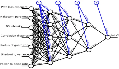
case of HCPP. The input features of the neural network are the network parameters and the output features are the elements of parameter vector β; see Fig. 3. The proposed NN is composed ofM layers withNmbeing the number of neurones of the mth layer. .

A. Dataset Construction

In order to train our NN, we need to build a dataset. For this, we run a large number of simulations with various network setups, i.e different values of θ. For each scenario, we compute, using Monte Carlo (MC) simulations, the corresponding coverage for the typical values of the SINR threshold τdB ∈ [−30,30] dB.

By fitting the model described in equation (4) to the obtained coverage results, we collect the vector β that matches the studied scenario. By the end of this iterative process, we obtain the desired dataset. Table. I gives an idea about how our dataset is structured in the case of PPP networks; values of the network features are randomly drawn from the the typical intervals shwon in Table. II. Our dataset is constructed using Matlab and Simulink curve-fitting tools.

The generated dataset, denoted byS, consists of

S ={(θ(1),β(1)), . . . ,(θ(n),β(n))}, (5)

where θ(j) andβ(j) denote respectively thej-th input andj-th output feature vectors, andnis the size of the dataset. The dataset is randomly split between a training set, which represents 80% of the entire dataset, and test set.

B. Cost function

The cost function allows to tune the NN parameters, denoted by vectorψ, in order to obtain the best match-ing between the actual and predicted outputs. We choose

Path loss exponent

Nakagami parameter

Radius of guard zone

Shadowing variance Power-to-noise ratio BS intensity Correlation distance −0.30301 −0. 5863

−0.47 76 −1. 5648 5 −1. 0040 10.55699 1.69634 0.90 936 −0. 6401 1 0.02 439

−2.₇₃₀ 81 0.03771 0.955 35 2.03 583 1.78 739 − 0.1₄₇ 66 0.03 346 −1.27942 −1.06

874 1.54 712 0.3 63 62 − 0.5₄₄ 15 −1.477 48 0.43977 0.020 95 − 1.0₀₅ 67 0.4 20₅₆ −_1.5 145 −0.1631 −0.75095 1.8 72 11 0.1₀₅ 17 1.3 26₂₈ 0.₄₄₈ 38 −0.9591 0.15026 0.39 547 −0. 2780 8 −0.55376 1.82 339 −0. 3927 2 − 1.4₂₂ 0.51381 0.98 622 1.3 565 0.3₂₆ 71 1.02019 − 0.0₁₅ 39 − 0.3₉₇ 09 −0.31432 −1.10419 −0. 7115 4 −_0.7 43₆₂ −0.65

679 −

1.7 84₇₄

−3.08575

−0.1814 6 1.1₁₈ 6 beta2 0.6 35 98 − 0.0 29 37 0.1 69 79 0.2₀₉ 64 −_1.27 06 1 1.627 34 2.0 982 0.3 42₂₄ 1 − 3.0 053 1 0.5₆₇ 38 1 − 0.0 46 36 1

Error: 0.002581 Steps: 44

beta2

Fig. 3: Neural networks plots forβ2estimation.

this to be the conventional mean square error (MSE), given by the following expression

J(ψ) = X

k∈NT

kβ(k)−f(θ(k);ψ)k2. (6)

wheref(θ(k)_{;ψ)is the output of the NN to inputθ}(k)

and thus the estimate of β(k), and NT refers to the training dataset. The optimum NN parameter vector ψ

is obtained by minimizing the above cost function using a retropropagation algorithm.

C. Neural network model

Different neural networks are implemented using

neuralnetpackage in R studio. Comparing the different NN models, we observed that a three-layer NN is sufficient to achieve very high accuracy, and having more than three layers did not significantly improve the prediction accuracy.

In the case of PPP networks, after convergence, the part of the NN which predicts β2 is shown in Fig. 3.

D. Accuracy results

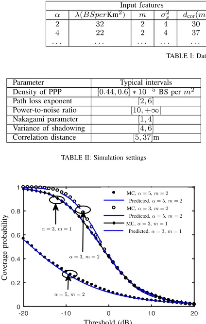
In order to illustrate the accuracy of the NN-base modeling, we select some PPP network scenarios and depict in Figure 4 the estimated coverage (based on Monte Carlo simulations) and the NN-based coverage probability prediction. As shown in the figure, the NN-based model provides a very accurate prediction of the coverage probability.

V. CONCLUSION

Input features Output vector

α λ(BSperKm2

) m σ2

s dcor(m) γ β0 β1 β2

2 32 2 4 30 10 −3.57 −0.0763 8.05∗10−5

4 22 2 4 37 ∞ −2.72316444 −0.03 0.0005

. . . .

TABLE I: Dataset sample forp= 2.

Parameter Typical intervals

Density of PPP [0.44,0.6]∗10−5 _{BS perm}2

Path loss exponent [2,6]

Power-to-noise ratio [10,+∞[

Nakagami parameter [1,4]

Variance of shadowing [4,6]

Correlation distance [5,37]m

TABLE II: Simulation settings

-20 -10 0 10 20

0 0.2 0.4 0.6 0.8 1

C

o

v

er

ag

e

p

ro

b

ab

il

it

y

Threshold (dB)

α= 3,m= 1

α= 3,m= 2

α= 5,m= 2

MC,α= 5,m= 2

Predicted,α= 5,m= 2

Predicted,α= 5,m= 2

MC,α= 3,m= 2

MC,α= 3,m= 1

Predicted,α= 3,m= 1

Fig. 4: Predicted coverage vs Monte Carlo simulations. For these simulations,

λ= 4.4∗10−6_{BS perm}2_,d

cor= 37m,σ 2

=−100dB,Pb= 1mW.

based on the gamma approximation of the interference distribution.

VI. ACKNOWLEDGMENT

This work has been partly funded by VLIR-UOS. We thank Prof. Pollin from KU Leuven for her valuable feedback on earlier versions of this paper.

REFERENCES

[1] H. ElSawy, A. Sultan-Salem, M.-S Alouini Alouini, and M. Z. Win, “Modeling and analysis of cellular networks using

stochas-tic geometry: A tutorial,” IEEE Communications Surveys and

Tutorials, vol. 19, no. 1, pp. 167–203, 2017.

[2] J. Andrews, F. Baccelli, and R. K. Ganti, “A tractable approach

to coverage and rate in cellular networks,” IEEE Transactions

on Communications, vol. 59, no. 11, pp. 3122–3134, 2011.

[3] Martin Haenggi and Radha Krishna Ganti,Interference in large

wireless networks, Now Publishers Inc, 2009.

[4] H. ElSawy, A. Hossain, and M. Haenggi, “Stochastic geometry for modeling, analysis, and design of multi-tier and cognitive

cellular wireless networks: A survey,” IEEE Communications

Surveys & Tutorials, vol. 15, no. 3, pp. 996–1019, 2013. [5] H. ElSawy, H. Ekram, and M.-S Alouini Alouini, “Analytical

modeling of mode selection and power control for underlay d2d

communication in cellular networks,” IEEE Transactions on

Communications, vol. 62, no. 11, pp. 4147–4161, 2014. [6] Martin Haenggi, “The meta distribution of the sir in poisson

bipolar and cellular networks,” IEEE Transactions on Wireless

Communications, vol. 15, no. 4, pp. 2577–2589, 2016.

[7] M. Mozaffari, W. Saad, M. Bennis, and M. Debbah, “Mobile internet of things: Can uavs provide an energy-efficient mobile

architecture?,” in IEEE Global Communications Conference

(GLOBECOM), Washington DC, USA, Dec. 2016, pp. 1–6.

[8] F. Baccelli and X. Zhang, “A correlated shadowing model

for urban wireless networks,” in 2015 IEEE Conference on

Computer Communications (INFOCOM), 2015, pp. 801–809. [9] S. Szyszkowicz, F. Alaca, H. Yanikomeroglu, and J.

Thomp-son, “Aggregate interference distribution from large wireless networks with correlated shadowing: An analytical–numerical–

simulation approach,”IEEE Transactions on Vehicular

Technol-ogy, vol. 60, no. 6, pp. 2752–2764, 2011.

[10] R. W Heath, M. Kountouris, and T. Bai, “Modeling hetero-geneous network interference using poisson point processes,”

IEEE Transactions on Signal Processing, vol. 61, no. 16, pp. 4114–4126, 2013.

[11] A. Guo and M. Haenggi, “Spatial stochastic models and metrics

for the structure of base stations in cellular networks,” IEEE

Transactions on Wireless Communications, vol. 12, no. 11, pp. 5800–5812, 2013.

[12] Ali Mohammad Hayajneh, Syed Ali Raza Zaidi, Des C McLer-non, and Mounir Ghogho, “Performance analysis of uav enabled disaster recovery network: a stochastic geometric framework

based on matern cluster processes,” IEEE Access, 2017.

[13] Vasant Dhar, “Data science and prediction,” Communications

of the ACM, vol. 56, no. 12, pp. 64–73, 2013.

[14] S. Han, I. Chih-Lin, G. Li, S. Wang, and Q. Sun, “Big data

enabled mobile network design for 5G and beyond,” IEEE

Communications Magazine, vol. 55, no. 9, pp. 150–157, 2017. [15] M. Kulin, C. Fortuna, E. De Poorter, D. Deschrijver, and I. Mo-erman, “Data-driven design of intelligent wireless networks: An

overview and tutorial,” Sensors, vol. 16, no. 6, pp. 790, 2016.

[16] J. Herzen, H. Lundgren, and N. Hegde, “Learning Wi-Fi

performance,” in Annual IEEE International Conference on

Sensing, Communication, and Networking (SECON), 2015, pp. 118–126.

[17] A. Samba, Y. Busnel, A. Blanc, P. Dooze, and G. Simon, “Throughput prediction in cellular networks: Experiments and

preliminary results,” in 1`eres Rencontres Francophones sur

la Conception de Protocoles, l’ ´Evaluation de Performance et l’Exp´erimentation des R´eseaux de Communication (CoRes 2016), 2016.

[18] D. T. Delaney and G. M. O’Hare, “A framework to implement IoT network performance modelling techniques for network

solution selection,” Sensors, vol. 16, no. 12, pp. 2038, 2016.

[19] Y. Lin, E. Oliveira, S. Jemaa, and S. Elayoubi, “Machine learn-ing for predictlearn-ing QoE of video streamlearn-ing in mobile networks,” in IEEE International Conference on Communications (ICC), 2017, pp. 1–6.

[20] J. Chen, U. Yatnalli, and D. Gesbert, “Learning radio maps for UAV-aided wireless networks: A segmented regression

ap-proach,” inIEEE International Conference on Communications

(ICC), 2017.

[21] N. Alotaibi and S. Alwakeel, “A neural network based handover

management strategy for heterogeneous networks,” in

Inter-national Conference on Machine Learning and Applications (ICMLA), 2015, pp. 1210–1214.

[22] J. Kim, J Park, J. Noh, and S. Cho, “Completely

dis-tributed power allocation using deep neural network for device

to device communication underlaying LTE,” arXiv preprint

arXiv:1802.02736, 2018.