Compressive Sensing Based Image Processing
and Energy-Efficient Hardware Implementation
with Application to MRI and JPEG 2000
by
Nandini Ramesh Kumar
in fulfilment of the requirements of
PHD DISSERTATION
Faculty of Health,Engineering & Sciences
University of Southern Queensland
by
Nandini Ramesh Kumar
Abstract
In the present age of technology, the buzzwords are low-power, energy-efficient and compact systems. This directly leads to the date processing and hardware techniques employed in the core of these devices. One of the most power-hungry and space-consuming schemes is that of image/video processing, due to its high quality requirements. In current design methodologies, a point has nearly been reached in which physical and physiological effects limit the ability to just encode data faster. These limits have led to research into methods to reduce the amount of acquired data without degrading image quality and increasing the energy con-sumption.
Compressive sensing (CS) has emerged as an efficient signal compression and re-covery technique, which can be used to efficiently reduce the data acquisition and processing. It exploits the sparsity of a signal in a transform domain to perform sampling and stable recovery. This is an alternative paradigm to conventional data processing and is robust in nature. Unlike the conventional methods, CS provides an information capturing paradigm with both sampling and compres-sion. It permits signals to be sampled below the Nyquist rate, and still allowing optimal reconstruction of the signal. The required measurements are far less than those of conventional methods, and the process is non-adaptive, making the sampling process faster and universal.
reduces the overall processing, and a faster computation when combined with CS.
Considering the requirements, this thesis is presented in two parts. In the first part: (1) A complex Hadamard matrix (CHM) based 2D and 3D MRI data acquisition with recovery using a greedy algorithm is proposed. The CHM mea-surement matrix is shown to satisfy the necessary condition for CS, known as restricted isometry property (RIP). The sparse recovery is done using compres-sive sampling matching pursuit (CoSaMP); (2) An optimized matrix and modified CoSaMP is presented, which enhances the MRI performance when compared with the conventional sampling; (3) An energy-efficient, cost-efficient hardware design based on field programmable gate array (FPGA) is proposed, to provide a plat-form for low-cost MRI processing hardware. At every stage, the design is proven to be superior with other commonly used MRI-CS methods and is comparable with the conventional MRI sampling.
Certification of Dissertation
I certify that the ideas, designs and experimental work, results, analyses and conclusions set out in this dissertation are entirely my own effort, except where otherwise indicated and acknowledged.
I further certify that the work is original and has not been previously submitted for assessment in any other course or institution, except where specifically stated.
Nandini Ramesh Kumar
0050109401
Signature of Candidate
Date
ENDORSEMENT
Signature of Supervisor/s
First and foremost, I would like to express my gratitude to my principal super-visor A/Prof. Wei Xiang. My research would not have been possible without his support and guidance. I am thankful to my associate supervisor A/Prof. John Leis, for his support during my PhD tenure.
I would also like to thank USQ for providing a three-year post graduate research scholarship, without which my research term would be hectic. Also, thanks to the Computational Engineering and Science Research Centre (CESRC) for the top-up scholarship. A heartfelt thanks to my colleagues, who have extended their knowledge and resources in MRI. It would have been difficult to complete my thesis without these resources. The discussions that we had are invaluable. Special thanks to Ms. Juanita Ryan, who has always been there and extended unconditional support whenever needed. Thanks to my friends and family, for having faith in my capabilities. Their constant motivation and support has given me the confidence to do this research.
Last, but not the least, I would like to thank and dedicate this thesis to my husband Ramesh, who has been my pillar of strength. I am greatly indebted for his unconditional love, patience and all the sacrifices, even though it has not been easy being away from family and friends. A big thankyou to my friends in Toowoomba, for helping me stay positive and giving me the ‘can do’ attitude.
Nandini Ramesh Kumar
Associated Publications
The following publications were produced during the period of candidature:
[1] Nandini Ramesh Kumar, Wei Xiang and Yafeng Wang, “An FPGA-based fast two-symbol processing architecture for JPEG 2000 arithmetic coding”, in
Proc. 35th International Conference on Acoustics, Speech, and Signal Processing (ICASSP), 14-19 Mar. 2010, Dallas, TX. USA, pp. 1282-1285.
[2] Nandini Ramesh Kumar, Wei Xiang and Yafeng Wang, “Two-symbol FPGA architecture for fast arithmetic encoding in JPEG 2000”, Journal of Signal Pro-cessing Systems, Vol. 69, No. 2, pp. 213-224, 2012.
The work in these papers is presented in Chapter 7.
[3] Nandini Ramesh Kumar, Wei Xiang and Jeffrey Soar, “A Novel Image Com-pressive Sensing Method Based on Complex Measurements”, in Proc. Inter-national Conference on Digital Image Computing Techniques and Applications (DICTA), 6-8 Dec. 2011, Noosa, QLD, AUSTRALIA, pp. 175-179.
Abstract i
Acknowledgments iv
Associated Publications v
List of Figures xi
List of Tables xv
Acronyms & Abbreviations xvii
Chapter 1 Introduction 1
1.1 Research Problem . . . 2
1.2 Contributions . . . 4
1.3 Organization . . . 5
Chapter 2 Background 7
2.1 Compressive Sensing Theory . . . 7
2.1.1 Sparsity . . . 8
CONTENTS vii
2.1.3 CS Recovery Algorithms . . . 12
2.1.4 CS Recovery Guarantees . . . 14
2.1.5 Structure of CS Matrices . . . 15
2.2 Magnetic Resonance Imaging . . . 18
2.2.1 Imaging . . . 20
2.2.2 Image Acquisition . . . 21
2.2.3 Non-Fourier MRI Mathematical model . . . 22
2.3 CS-based MRI Processing . . . 24
2.4 Image Processing with JPEG 2000 . . . 24
2.5 Field Programmable Gate Array Architecture . . . 26
Chapter 3 2D and 3D MRI Processing Using CS-Based Complex Measurements 28 3.1 Introduction . . . 28
3.2 Related Work . . . 29
3.3 Compressive Sensing for 2D and 3D MRI . . . 30
3.3.1 Complex Hadamard Matrix . . . 31
3.3.2 Computational Complexity . . . 36
3.4 Numerical Results . . . 37
3.4.1 Simulations for 2D-MRI . . . 38
3.4.2 Simulations for 3D-MRI . . . 42
3.5 Summary . . . 49
En-hanced 2D/3D-MRI Performance 50
4.1 Related Work . . . 51
4.2 Matrix Formulation . . . 51
4.3 Restricted Isometry Property . . . 52
4.3.1 Complex Hadamard based CoSaMP . . . 55
4.4 Numerical Results . . . 57
4.4.1 Simulation Results for 2D MRI . . . 58
4.4.2 Simulation Results for 3D MRI . . . 59
4.5 Summary . . . 61
Chapter 5 Computation Efficient FPGA-Based Hardware Archi-tecture for MRI Processing 62 5.1 Introduction . . . 62
5.2 Related Work . . . 63
5.3 System Architecture . . . 64
5.4 Hardware Process . . . 65
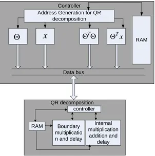
5.4.1 QR Decomposition for Complex Hadamard Matrix . . . . 68
5.4.2 Data Processing on Hardware . . . 68
5.5 Simulation Results . . . 70
5.6 Practical Application . . . 72
5.7 Summary . . . 72
Chapter 6 Low-complexity Energy-Efficient CS-based Natural
CONTENTS ix
6.1 Introduction . . . 73
6.2 Related Work . . . 74
6.3 System Model . . . 76
6.4 CS Processing . . . 77
6.5 Hardware Architecture . . . 78
6.5.1 Encoder . . . 78
6.5.2 Decoder . . . 80
6.5.3 Energy-efficient Processing . . . 82
6.6 Numerical Results . . . 86
6.7 Summary . . . 89
Chapter 7 Two-symbol Arithmetic Encoding Architecture For Ef-ficient Entropy Coding in CS-Based JPEG 2000 90 7.1 Introduction . . . 90
7.2 Related Work . . . 91
7.3 Arithmetic Encoding System Model . . . 92
7.4 Two-symbol Arithmetic Encoding Architecture . . . 97
7.4.1 Interval Update Stage . . . 97
7.4.2 Code Update Stage . . . 98
7.4.3 Probability Estimation Table and State Update . . . 101
7.4.4 Index Prediction . . . 101
7.4.5 Critical Path Analysis . . . 101
7.6 Simulation Results . . . 102
7.7 Summary . . . 106
Chapter 8 Conclusions 107
8.1 Future Work . . . 108
List of Figures
2.1 Illustration of 3D-MRI encoding directions. . . 23
2.2 Performance comparison of JPEG 2000 vs. JPEG. . . 25
2.3 JPEG 2000 encoder block diagram. . . 26
2.4 Internal structure of an ALM. . . 27
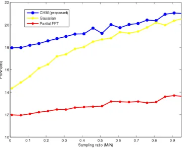
3.1 Rate distortion performance of various measurement matrices. . . 39
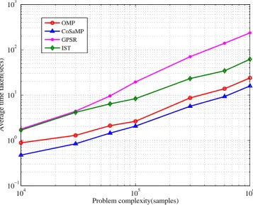
3.2 Runtime performance of reconstruction methods with respect to image complexity. . . 40
3.3 Reconstructed data for a 256×256 angio MRI image with 4K sam-ples (from (b) to (d)) and 10K samsam-ples (from (f) to (h)) . . . 40
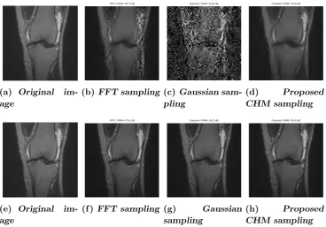
3.4 Reconstructed data for a 256×256 knee MRI image with 4K sam-ples (from (b) to (d)) and 10K samsam-ples (from (f) to (h)). . . 41
3.5 Reconstructed data for a 256×256 spine MRI image with 4K sam-ples (from (b) to (d)) and 10K samsam-ples (from (f) to (h)). . . 41
3.6 3D Shepp-Logan phantom of size 256× 256× 11. Fig.1(a) is a single 2D original slice and Fig.1(b) shows the reconstruction from our proposed method. . . 43
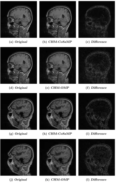
3.8 Fully sampled and reconstructed images for a 256×256 single 2D slice of a 3D dataset. The Ψ matrix used is the identity matrix and CHM is the Φ matrix. The reconstruction is performed with
CoSaMP as in Fig(b) and with OMP as in Fig (c). . . 46
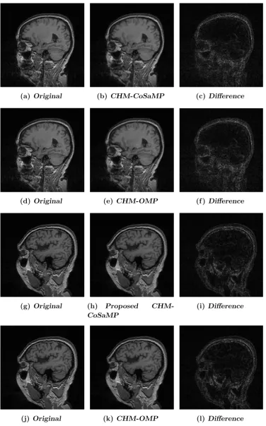
3.9 Fully sampled and reconstructed images for a 256×256 single 2D slice of a 3D dataset. The Ψ matrix used is the Daubechies-4 wavelet and CHM is the Φ matrix. The reconstruction is performed with CoSaMP as in Fig(b) and with OMP as in Fig (c). . . 47
3.10 Reconstructed 3D-MRI model from fully sampled and Proposed methods. . . 48
3.11 Reconstructed 3D-MRI model from fully sampled and Proposed methods. . . 48
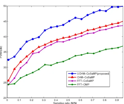
4.1 PSNR versus sampling rate graph comparing the proposed UCHM, CHM proposed in Chapter 3, FFT with CoSaMP reconstruction and FFT with OMP used in Chapter 3. Daubechies-4 wavelet is used as the matrix Φ . . . 57
4.2 Fully sampled and reconstructed images with 10K measurements for a 256×256 ‘angio’ 2D-MRI image. . . 58
4.3 Fully sampled and reconstructed images with 10K measurements for a 256×256 ‘knee‘ 2D-MRI image. . . 58
4.4 Fully sampled and reconstructed images with 10K measurements for a 256×256 ‘spine‘ 2D-MRI image. . . 59
4.5 Fully sampled and reconstructed images with 20K measurements for a 256×256 single 2D slice of 3D dataset-1. . . 60
4.6 Fully sampled and reconstructed images with 20K measurements for a 256×256 single 2D slice of 3D dataset-2. . . 60
5.1 Architecture of the hardware reconstruction process. . . 65
5.2 Block diagram for MRI hardware processing. . . 65
5.3 Internal structure of the reconstruction process. . . 67
LIST OF FIGURES xiii
5.5 Reconstructed images of a two slices ((a) and (d))from a total MRI
scan samples of dataset-2 [1]. . . 70
6.1 System model with for CS processing. . . 76
6.2 Flow chart for the proposed encoder architecture. . . 79
6.3 Detailed block diagram of the proposed encoder. . . 79
6.4 9/7 lifting wavelet structure. α,β,γ andδare the lifting parameters. 80 6.5 Timing diagram of DWT with CS. . . 80
6.6 Block diagram of the proposed decoder. . . 81
6.7 Inverse lifting wavelet structure. . . 82
6.8 Timing diagram of the decoder. . . 82
6.9 Graph showing power consumption with various FPGA storage options. . . 83
6.10 16K ×8 bits memory mapping without selection logic. . . 83
6.11 16K×8 bits memory mapping with banking and address selection logic. . . 84
6.12 Single processing element (PE) of a multiplication block. . . 85
6.13 Original and reconstructed test images. . . 87
6.14 Original and reconstructed output of a 256×256 image-1. . . 88
6.15 Original and reconstructed output of a 256×256 image-2. . . 88
6.16 Original and reconstructed output of a 256×256 image-3. . . 88
7.1 Interval length division. . . 94
7.2 AE flowchart. . . 94
7.4 (a) Renormalization flowchart; (b) Byte-out flowchart; and (c) Flush procedure flowchart. . . 96
7.5 Block diagram of the proposed two-symbol AE architecture. . . . 97
7.6 Interval (A) Update procedure. . . 98
7.7 Code (C) Update procedure. . . 99
7.8 (a) Register C update module; (b) Mask Generation module. . . . 100
List of Tables
3.1 Computational complexity of some popular CS reconstruction al-gorithms used for MRI. The complexity is based on aM×N matrix for ak-sparse basis, u is the median filter andα is the redundancy. 37 3.2 PSNR performance comparison for 256×256 test images with 4K
measurements. . . 42
3.3 PSNR performance comparison for 256×256 test images with 10K measurements. . . 42
3.4 Comparison of number of iterations and corresponding P SN Rm
for proposed method and NFCS-3D [2]. The acceleration factors vary from 4 to 16 times. . . 44
3.5 PSNR performance for dataset-1. . . 45
3.6 PSNR performance for dataset-2. . . 48
4.1 PSNR performance 2D-MRI images with 10K measurements. . . . 59
4.2 PSNR performance 3D dataset-1. . . 59
4.3 PSNR performance 3D dataset-2. . . 60
5.1 Hardware comparison with existing CS reconstruction architectures. 71
6.1 Computational complexity for CHM, random FFT, random Gaus-sian in block processing. The complexity is based on a M ×N
matrix for a k-sparse basis. CoSaMP reconstruction is used in all cases. . . 86
6.3 PSNR performance of various test images considered. . . 89
7.1 Hardware implementation cost. . . 103
7.2 Number of clock cycles for 512×512 image, code block size 64×64, lossless compression. . . 103
7.3 Frequency and throughput comparison among the proposed two-symbol architecture and other one-two-symbol and two-two-symbol archi-tectures in the literature. . . 104
Acronyms & Abbreviations
2D Two Dimensional
3D Three Dimensional
AE Arithmetic Encoding ALM Adaptive Logic Module ALUT Adaptive Look-Up Table AMD Advanced Micro Devices
ASIC Application Specific Integrated Circuit BC Bit-plane Coding
BP Basis Pursuit
BPC Bit Plane Coder
BPDN Basis Pursuit DeNoising
BPIC Basis Pursuit with Integrated Constraints CG Conjugate Gradient
CHM Complex Hadamard Matrix
CORDIC COordinate Rotation DIgital Computer CoSaMP Compressive Sampling Matching Pursuit CPC Column Processing Core
CPU Central Processing Unit
CRAD Complex RADemacher function
CRAM Configuration Random Access Memory CS Compressive Sensing
CX-D Context-Decision (pair) DCT Discrete Cosine Transform DWT Discrete Wavelet Transform
EBCOT Embedded Block Coding with Optimized Truncation FFT Fast Fourier Transform
FIFO First In First Out
FPGA Field Programmable Gate Array
FOCUSS FOCal Underdetermined System Solution FOV Field Of View
GHz Giga Hertz
ICBM International Consortium of Brain Mapping IDWT Inverse Discrete Wavelet Transform
IHT Iterative Hard Thresholding IST Iterative Shrinkage/Thresholding JPEG Joint Pictures Expert Group LPS Least Probable Symbol LUT Look-Up Table
MHz Mega Hertz
MP Matching Pursuit MPS Most Probable Symbol
MRA Magnetic Resonance Angiography MRI Magnetic Resonance Imaging MSB Most Significant Bit
NLPS Next Least Probable Symbol NMR Nuclear Magnetic Resonance NMPS Next Most Probable Symbol OMP Orthogonal Matching Pursuit PE Processing Element
PFFT Partial Fast Fourier Transform POCS Projection Onto Convex Set PSNR Peak Signal-to-Noise Ratio QRD matrix Q and R Decomposition RAM Random Access Memory
RF Radio Frequency
RIP Restricted Isometry Property RPC Row Processing Core
SART Simultaneous Algebraic Reconstruction Technique SNR Signal-to-Noise Ratio
SP Subspace Pursuit
TSMC Taiwan Semiconductor Manufacturing Company TV Total Variation
Chapter 1
Introduction
Information processing is a dominant part in any field that uses present tech-nologies. Computational and analytical tools are being continuously developed for the extraction of information from data, and are fast becoming irrelevant in the face of large problem sizes necessitated by todays applications. Therefore, the challenge is to devise new and computationally efficient set of information processing tools that can effectively cope with this huge set of data.
1.1
Research Problem
In present clinical practice, magnetic resonance imaging (MRI) is one of the most popular imaging modalities due to its excellent depiction of soft tissues, and inherent absence of emitted ionizing radiation. The traditional approach of MRI data acquisition is to sample at Nyquist rate followed by use of coding methods for compression. Recent trends have advanced to 3D-MRI and generally require faster acquisition techniques to achieve clinical practicality. Unfortunately, such accelerations may result in a compromise of image quality, in terms of spatial and temporal resolution, signal-to-noise ratio (SNR) etc.
Despite its many advantages, a fundamental limitation of MRI is the linear rela-tion between the number of measured data samples and net scan time. Increased scan duration presents a number of practical challenges in clinical imaging in-cluding higher susceptibility to physiological motion artifacts, diminished clinical throughput, and added patient discomfort. This shows the importance of imaging speed in MRI applications. However, the speed at which data can be collected in MRI is fundamentally limited by physical (gradient amplitude and slew-rate) and physiological (nerve stimulation) constraints [3]. Therefore, the prime concern is to seek methods to reduce the amount of acquired data without degrading the image quality.
In the past several years, the practical performance of CS theory, has been suc-cessfully demonstrated for a large range of clinical applications including non-Cartesian and 3D-MR angiography (MRA) [3,4], and time-resolved imaging [5]. Several groups in the MRI community have proposed novel numerical techniques for robust CS with specific focus on MR image reconstruction including nonlinear conjugate gradient (CG) [3], interior point (IP) [6], Bregman iteration or inverse scale space [7], and iterative reweighted least squares or FOCUSS [8,9] methods. Since there has been very few comparison of the computational performance of these techniques on large-scale problems to date, the best approach that can meet the clinical demands is still an open question. Moreover, to improve the speed, it becomes necessary that the processing algorithms are also computationally sped up. There have various attempts where central processing unit (CPU), graphic processing unit (GPU), field programmable gate array (FPGA) and application specific integrated circuit (ASIC) [10–15] being used for this purpose, which have time durations ranging from minutes to hours. Again, though there are solutions for reduction in computation time, the desire for the least computational time needs to be ascertained.
1.1 Research Problem 3
transform coefficients are retained, while most of the other sampled data will be discarded. This is further entropy encoded, particularly in JPEG 2000, which is a cumbersome process. All the data is entropy encoded bit-by-bit and this leads to a slower system and high complexity. Hence, combining CS with image encoder can be one solution that could lead to having very few data transformed data (e.g., less than 10%) when compared to conventional image transforms. It is a known fact that, due to CPU dependencies, software-based processing is much slower than hardware-based processing. Moreover, with modern image/video technologies low-complexity, low-energy and small-size hardware systems are most preferable. This, further adds up to the necessity of having a image encode-decode system that addresses the aforementioned issues.
Considering the issues related to MRI and natural imaging, a solution is nec-essary that will help in overcoming these issues. This points to compressive sensing, which has been successful in providing reconstruction of data from very few samples. This study focusses on applying CS techniques for encoding and reconstruction, in order to overcome the drawbacks persisting in MRI and natural imaging. Specifically, this work focuses on; i) To reduce the MRI data acquisition without compromising quality of the processed data and; ii) CS-based JPEG 2000 optimized system that provides a high compression ratio and image quality, and also have a low-complexity and low-energy consumption.
1.2
Contributions
The primary essence of this work is to provide a low-complexity, low-cost, energy-efficient encoding-decoding system for MRI and natural imaging, while overcom-ing the processovercom-ing speed issues. Though the application of CS techniques varies for MRI and natural imaging, the core CS principles are same. In case of MRI processing, CS is used for data acquisition and reconstruction of images. For CS-based natural imaging, the aim is to reduce the transform data and embed the CS principles in JEPG 2000.
Specifically the contributions are summarized as follows:
1. 2D and 3D MRI processing using CS-based complex measure-ments: A non-Fourier based 2D and 3D MRI data acquisition and recon-struction is designed. To enable CS techniques in this work, a complex Hadamard matrix proposed. This structure is used for the first time in this work and is elaborated in Chapter 3. The data acquisition is performed us-ing complex Hadamard matrix and the transform used is the Daubechies-4 wavelet [16]transform since they are highly incoherent. The combination of the complex Hadamard and wavelet transform, called the sensing matrix is shown to satisfy restricted isometry property. A specific bound for CoSaMP reconstruction is derived with respect to 3D-MRI. This bound is optimized for 3D-MRI performance. Furthermore, comparison is drawn with an ex-isting non-Fourier 3D CS algorithm. The simulation platform is built and performance of the system is shown in terms of signal-to-noise ratio. This method is discussed in Chapter 3.
2. Optimization of Complex Hadamard Matrix for Enhanced 2D/3D-MRI Performance: Chapter 4 mainly deals with the optimization algo-rithm and its effectiveness for 3D-MRI. An optimized version of the com-plex Hadamard matrix is presented and verified for CS properties, which is the primary requirement for any matrix to be used for CS-based pro-cessing. This is primarily a structured unitary matrix and hence termed as unitary complex Hadamard matrix. Furthermore, when used with the optimized CoSaMP(discussed in Chapter 3), ensures an enhanced 3D-MRI reconstruction. The numerical results are demonstrated for 3D-MRI and a comparison shows a significant increase in signal-to-noise ratio.
signal-1.3 Organization 5
to-noise ratio as when done through software methods. A comparison with other existing architectures, shows the efficiency of this architecture.
4. Low-complexity energy-efficient CS-based natural image process-ing hardware: A low-complex and energy-efficient pipelined hardware-based architecture is presented in Chapter 6. The main aim is to provide an architecture that can fit easily with the existing JPEG 2000 and is based on CS principles. The idea behind the use of CS is to drastically reduce the transform coefficients. This in turn makes the encoder less complex and easily portable on low-power devices.
5. Two-symbol arithmetic encoding architecture for efficient entropy coding in CS-based JPEG 2000: Chapter 7 mainly deals with entropy encoding. Here, a high-performance two-symbol arithmetic encoding hard-ware is presented. Most of the JPEG 2000 entropy coders are based on processing one symbol per clock cycle. This bit-by-bit serial operation is computationally intense and requires huge hardware resources. Alongside, the energy efficiency is goes down significantly due to its serial nature. This issue is dealt with in this chapter and results compared with some of the existing hardware architectures.
1.3
Organization
This dissertation begins with a review on the relevant topics used in this work in Chapter 2. This includes compressive sensing, magnetic resonance imaging, field programmable gate arrays and JPEG 2000. Chapters 3, 4 and 5 deal with CS-based MRI processing, optimizations and their hardware architecture design. Chapters 6 and 7 are mainly on JPEG 2000 hardware architecture design and application of CS for an improved efficiency.
In Chapter 3 a CS-based MRI processing method is detailed, by deriving a proof for restricted isometry property and bound for CoSaMP. Simulation results for both 2D-MRI and 3D-MRI are presented separately, in Sections 3.4.1 and 3.4.2, respectively.
Chapter 4 deals with optimizing the earlier proposed matrix and reconstruction algorithm, for an enhanced 3D-MRI performance. The derivation for the re-stricted isometry property is given in Section 4.3. Finally, the simulation results and discussions are presented in Section 4.4.
in Section 5.3. Again, for the purpose of validation and comparison, simulations results are shown in Section 5.5 and followed with discussions.
Chapter 6 details on the aspects of the hardware structure of the transform block of JPEG 2000 combined with CS techniques. The system model is presented in Section 6.3 and the related CS processing is detailed in Section 6.4. The designed hardware architecture with the details of pipelining and timing diagrams are presented in Section 6.5, for both encoder and decoder. The simulated results are discussed in Section 6.6.
In Chapter 7, a two-symbol arithmetic encoder for JPEG 2000 is presented. The detailed architecture and process is explained in Sections 7.3 and 7.4. The com-bined JPEG 2000 architecture from the Chapters 6 and 7 is shown Section 7.5, which is targeted for an FPGA. The simulation results for the arithmetic encoder is tabulated in Section 7.6.
Chapter 2
Background
In this chapter, an overview of various theoretical aspects dealt in this thesis are provided. In Section 2.1, a brief description on compressive sensing theory is provided. In Section 2.2 we discuss magnetic resonance imaging with respect to single slice and 3D MRI. Section 2.5 and 2.4 provide an overview of the field programmable gate arrays and JPEG 2000 image processing, respectively.
2.1
Compressive Sensing Theory
Compressed sensing (CS) [17–20] offers a framework for simultaneous sensing and compression of finite-dimensional vectors, that rely on the reduction of linear dimensions. Specifically, in CS we do not acquire signal x directly but rather acquire M < N linear measurements y = Φx using an M ×N CS matrix Φ, where y is the measurement vector. Ideally, the matrix Φ is designed to reduce the number of measurements M as much as possible while allowing the recovery of a wide class of signals x from their measurement vectors y. However, the fact that M < N renders matrix Φ rank-deficient, meaning that it has a non-empty nullspace. This in turn, implies that for any particular signalx0 ∈RN, an infinite
number of signals x will yield the same measurements y0 = Φx0 = Φx for the
chosen CS matrix Φ.
2.1.1
Sparsity
Sparsity is the signal structure behind many compression algorithms that employ transform coding, and is the most prevalent signal structure used in CS. Sparsity also has a rich history of applications in signal processing problems in the last century (particularly in imaging), including denoising, deconvolution, restoration etc [21–23].
To introduce the notion of sparsity, we rely on a signal representation in a given basis {ψi}Ni=1 for RN. Every signal x ∈ RN is representable in terms of N
co-efficients {θ}N
i=1 as x =
PN
i=1ψiθi; arranging the ψi as columns into the N ×N
matrix ψ and the coefficients θi into theN ×1 coefficient vector θ, we can write
succinctly that x =ψθ, with θ ∈ RN. Similarly, if we use ψ containingN
unit-norm column vectors of lengthLwithL×N (i.e.,ψ ∈RL×N), then for any vector
x ∈RL there exist infinitely many decompositions θ ∈
RN such that x=ψθ. In
a general setting, we refer to ψ as the sparsifying dictionary [24]. These concepts are extendable to complex signals as well [25,26]. We say that a signal x is K -sparse in the basis ψ if there exists a vector θ ∈ RN with only K N nonzero
entries such that x=ψθ. We call the set of indices corresponding to the nonzero entries the support of θ and denote it by supp(θ). We also define the set ΣK
that contains all signalsxthat areK-sparse. A K-sparse signal can be efficiently compressed by preserving only the values and locations of its nonzero coefficients, using O(Klog2N) bits: coding each of the K nonzero coefficients locations takes
log2N bits, while coding the magnitudes uses a constant amount of bits that
de-pends on the desired precision, and is independent of N. This process is known as transform coding, and relies on the existence of a suitable basis Ψ that renders signals of interest sparse or approximately sparse.
For signals that are not exactly sparse, the amount of compression depends on the number of coefficients of θ that we keep. Consider a signal x whose coefficients
θ, when sorted in order of decreasing magnitude, decay according to the power law
|θ(I(n))| ≤Sn−1/r, n= 1, . . . , N, (2.1) where I indexes the sorted coefficients. Due to the rapid decay of their coeffi-cients, such signals are well-approximated byK-sparse signals. The bestK-sparse approximation error for such a signal obeys
σψ(x, K) :=arg min x0∈Σ
K
kx−x0k2 ≤CSK−s, (2.2)
with s = 1r − 1
2 and C denoting a constant that does not depend on N [27].
That is, the signal’s best approximation error in an l2-norm sense, has a power
2.1 Compressive Sensing Theory 9
by hard thresholding the signal’s coefficients, so that only theK coefficients with largest magnitudes are preserved.
2.1.2
Design of Measurement Matrices
The main design criteria for the CS matrix Φ is to enable the unique identification of a signal of interestxfrom its measurementsy= Φx. Clearly, when we consider the class of K-sparse signals ΣK, the number of measurements M > K for any
matrix design, since the identification problem has K unknowns even when the support Ω =supp(x) of the signal x is provided. In this case, we simply restrict the matrix Φ to its columns corresponding to the indices in Ω, , denoted by ΦΩ,
and then use the pseudoinverse to recover the nonzero coefficients of x:
xΩ = Φ
†
Ωy. (2.3)
Here xΩ is the restriction of the vector x to the set of indices Ω, and M† =
(MT)−1MT denotes the pseudoinverse of the matrixM. The implicit assumption in (2.3) is that ΦΩ has full column-rank so that there is a unique solution to
y= ΦΩxΩ.
We begin by determining properties of Φ that guarantee that distinct signals
x, x0 ∈ ΣK, x 6= x0, lead to different measurement vectors Φx 6= Φx0. In other
words, we want each vectory=RM to be matched to at most one vector x∈ΣK
such that y = Φx. A key relevant property of the matrix in this context is its spark.
Definition 1. [28] The spark spark(Φ) of a given matrix Φ is the smallest number of columns of Φ that are linearly dependent.
The spark is related to the Kruskal Rank from the tensor product literature; the matrix Φ has Kruskal rank spark(Φ)−1. This definition allows us to pose the following straightforward guarantee.
Theorem 1. [28] If spark(Φ)>2K , then for each measurement vectory ∈RM
there exists at most one signal x∈ΣK such that y= Φx.
It is easy to see that spark∈[2, M+ 1], so that Theorem 1 yields the requirement
M ≥2K.
Definition 2. [29] The coherence µ(Φ) of a matrix Φ is the largest absolute inner product between any two columns of Φ:
µ(Φ) = max
1≤i6=j≤N
|hΦi,Φji|
||Φi||l2||Φj||2
(2.4)
It can be shown that µ(Φ) ∈ hq N−M
M(N−1),1
i
; the lower bound is known as the
Welch bound [30,31]. Note that whenN M, the lower bound is approximately
µ(Φ) ≥ 1/√M. One can tie the coherence and spark of a matrix by employing the Gershgorin circle theorem.
Theorem 2. [32] The eigenvalues of anm×m matrixM with entries Mi,j,1≤
i, j ≤ m, lie in the union of m discs di = di(ci, ri),1 ≤ i ≤ m, centered at
ci =Mi,i with radius ri = Σj6=i|Mi,j|.
Applying this theorem on the Gram matrix G = ΦT
ΩΦΩ leads to the following
result.
Lemma 1. [28] For any matrix Φ,
spark(Φ)≥1 + 1
µ(Φ). (2.5)
By merging Theorem 1 with Lemma 1, we can pose the following condition on Φ that guarantees uniqueness.
Theorem 3. [28,33,34] If
K < 1
2(1 + 1
µ(Φ), (2.6)
then for each measurement vector y∈RM there exists at most one signal x∈ΣK
such that y= Φx.
2.1 Compressive Sensing Theory 11
uniqueness; however, it is desirable for the measurement process to be tolerant to both types of error. To be more formal, we would like the distance between the measurement vectors for two sparse signals y= Φx, y0 = Φx0 to be proportional to the distance between the original signal vectors x and x0. Such a property allows us to guarantee that, for small enough noise, two sparse vectors that are far apart from each other cannot lead to the same (noisy) measurement vector. This behavior has been formalized into the restricted isometry property (RIP).
Definition 3. [37] A matrixΦhas the (K, δ)-restricted isometry property ((K, δ )-RIP) if, for all x∈ΣK,
(1−δ)kxk22 ≤ kΦxk22(1 +δ)kxk22. (2.7) In words, the (K, δ)-RIP ensures that all submatrices of Φ of size M ×K are close to an isometry, and therefore distance-preserving. We will show later that this property suffices to prove that the recovery is stable to presence of additive noise n. In certain settings, noise is introduced to the signalx prior to measure-ment. Recovery is also stable for this case; however, there is a degradation in the distortion of the recovery by a factor of N/M [38–40].
Furthermore, the RIP also leads to stability with respect to the multiplicative noise introduced by the CS matrix mismatch ∆ [35,36]. The RIP can be connected to the coherence property by using, once again, the Gershgorin circle theorem (Theorem 2).
Lemma 2. [41] If Φ has unit-norm columns and coherence µ = µ(Φ), then Φ
has the (K, δ)-RIP with δ≤(K−1)µ.
One can also easily connect RIP with the spark. For each K-sparse vector to be uniquely identifiable by its measurements, it suffices for the matrix Φ to have the (2K, δ)-RIP with δ > 0, as this implies that all sets of 2K columns of Φ are linearly independent, i.e., spark(Φ) > 2K (Theorems 1 and 3). We will see later that the RIP enables recovery guarantees that are much stronger than those based on spark and coherence. However, checking whether a CS matrix Φ satisfies the (K, δ)-RIP has combinatorial computational complexity.
Now that we have defined relevant properties of a CS matrix Φ, we discuss specific matrix constructions that are suitable for CS. AnM×N Vandermonde matrixV
constructed from N distinct scalars has spark(V) = M + 1 [27]. Unfortunately, these matrices are poorly conditioned for large values ofN, rendering the recovery problem numerically unstable. Similarly, there are known matrices Φ of size
M ×M2 that achieve the coherence lower bound
such as the equiangular tight frames [31]. It is also possible to construct
determin-istic CS matrices of sizeM×N that have the (K, δ)-RIP forK =O(√M logM/log(N/M)) [42]. These constructions restrict the number of measurements needed to recover a
K-sparse signal to beM =O(K2logN), which is undesirable for real-world values
of N and K. Fortunately, these bottlenecks can be defeated by randomizing the matrix construction. For example, random matrices Φ of sizeM×N whose entries are independent and identically distributed (i.i.d.) with continuous distributions have spark(Φ) = M + 1 with high probability. It can also be shown that when the distribution used has zero mean and finite variance, then in the asymptotic regime (as M andN grow) the coherence converges toµΦ = 2plogN/M [43,44]. Similarly, random matrices from Gaussian, Rademacher, or more generally a sub-gaussian distribution have the (K, δ)-RIP with high probability if
M =O(Klog(N/K)/δ2). (2.9) A Rademacher distribution gives probability 1/2 to the values ±1. A random variable X is called subgaussian if there exists c > 0 such that E(eXt) ≤ ec2t2/2
for allt ∈R. Examples include the Gaussian, Bernoulli, and Rademacher random variables, as well as any bounded random variable.
Finally, we point out that while the set of RIP-fulfilling matrices provided above might seem limited, emerging numerical results have shown that a variety of classes of matrices Φ are suitable for CS recovery, including subsampled Fourier and Hadamard transforms [45,46].
2.1.3
CS Recovery Algorithms
We now focus on solving the CS recovery problem, given y and Φ, find a signal
x within the class of interest such that y= Φx exactly or approximately. When we consider sparse signals, the CS recovery process consists of a search for the sparsest signal x that yields the measurements y. By defining the l0 norm of a
vector kxk0 as the number of nonzero entries in x, the simplest way to pose a
recovery algorithm is using the optimization
b
x= arg min
x∈RN
kxk0. (2.10)
Solving (2.10) relies on an exhaustive search and is successful for allx∈ΣK when
the matrix Φ has the sparse solution uniqueness property (i.e., for M as small as 2K). However, this algorithm has combinatorial computational complexity, since we must check whether the measurement vector y belongs to the span of each set of K columns of Φ, K = 1,2, . . . , N. Our goal, therefore, is to find computationally feasible algorithms that can successfully recover a sparse vectorx
from the measurement vectoryfor the smallest possible number of measurements
2.1 Compressive Sensing Theory 13
An alternative to the l0 norm used in (2.10) is to use the l1 norm, defined as
kxk1 =PNn=1|x(n)|. The resulting adaptation of (2.10), known as basis pursuit
(BP) [22], is formally defined as
b
x= arg min
x∈RNkxk1subjecttoy = Φx. (2.11)
Since the l1 norm is convex, (2.11) can be seen as a convex relaxation of (2.10).
Thanks to the convexity, this algorithm can be implemented as a linear program, making its computational complexity polynomial in the signal length [47]. The optimization (2.11) can be modified to allow for noise in the measurements y = Φx+n; we simply change the constraint on the solution to
b
x= arg min
x∈RNkxk1subjecttoky−Φxk2 ≤, (2.12)
where ≥ knk2 is an appropriately chosen bound on the noise magnitude. This
modified optimization is known as basis pursuit with inequality constraints (BPIC) and is a quadratic program with polynomial complexity solvers [47]. The La-grangian relaxation of this quadratic program is written as
b
x= arg min
x∈RN
kxk1+λky−Φxk2, (2.13)
and is known as basis pursuit denoising (BPDN). There exist many efficient solvers to find BP, BPIC, and BPDN solutions; for an overview, see [48]. Of-tentimes, a bounded-norm noise model is overly pessimistic, and it may be reasonable instead to assume that the noise is random. For example, addi-tive white Gaussian noise n ∼ N(0, σ2I) is a common choice. Approaches
de-signed to address stochastic noise include complexity-based regularization [49] and Bayesian estimation [50]. These methods pose probabilistic or complexity-based priors, respectively, on the set of observable signals. The particular prior is then leveraged together with the noise probability distribution during signal recovery. Optimization-based approaches can also be formulated in this case; one of the most popular techniques is the Dantzig selector [51]:
b
x= arg min
x∈RN
kxk1suchthatkΦT(y−Φx)k∞≤λ
p
logN σ, (2.14) wherek · k∞ denotes thel∞-norm, which provides the largest-magnitude entry in
a vector andλ is a constant parameter that controls the probability of successful recovery.
Algorithm 1 Orthogonal Matching Pursuit Input: CS matrix Φ, measurement vectory
Output: Sparse representation bx
Initialize:bx0,r =y, Ω =∅, i= 0
while halting criterion false do
i←i+ 1
b ←ΦTr {form residual signal estimate}
Ω = ΩS
supp(T(b,1)) {update support with residual} b
xi|Ω ←Φ
†
Ωy,bxi|ΩC ←0 {update signal estimate}
r ←y−Φbxi {update measurement residual}
end while
return bx←xbi
as Algorithm 1, where T(x, K) denotes a thresholding operator onx that sets all but the K entries of x with the largest magnitudes to zero, and x|Ω denotes the
restriction of x to the entries indexed by Ω. The convergence criterion used to find sparse representations consists of checking whether y = Φx exactly or ap-proximately; note that due to its design, the algorithm cannot run for more than
M iterations, as Φ has M rows. Other greedy techniques that are a similar, or rather derived from OMP include CoSaMP [53], and Subspace Pursuit (SP) [54]. Another variant is known as iterative hard thresholding (IHT) [55]: starting from an initial signal estimate bx0 = 0, the algorithm iterates a gradient descent step
followed by hard thresholding, i.e.,
b
x=T(bxi−1+ ΦT(y−Φbxi−1), K), (2.15)
until a convergence criterion is met.
2.1.4
CS Recovery Guarantees
Many of the CS recovery algorithms above come with guarantees on their per-formance. We group these results according to the matrix metric used to obtain the guarantee.
Theorem 4. [37,53–55] Let the signal x ∈ ΣK and write y = Φx+n. The
outputs bx of the CoSaMP, SP, IHT, and BPIC algorithms, with Φ having the
(cK, δ)-RIP, obey
kx−xbk2 ≤C1kx−xKk2+C2
1
√
Kkx−xKk1+C3knk2, (2.16)
where xK = arg minx0∈Σ
Kkx−x 0k
2 is the best K-sparse approximation of the
2.1 Compressive Sensing Theory 15
of the RIP and the values of C1, C2, and C3 are specific to each algorithm. For
example, for the BPIC algorithm, c = 2 and δ = √2−1 suffice to obtain the guarantee in (2.16).
The type of guarantee given in Theorem 4 is known as uniform instance optimal-ity, in the sense that the CS recovery error is proportional to that of the best
K-sparse approximation to the signalxfor any signalx∈RN. In fact, the
formu-lation of the CoSaMP, SP and IHT algorithms was driven by the goal of instance optimality, which has not been shown for older greedy algorithms like MP and OMP. Theorem 4 can also be adapted to recovery of exactly sparse signals from noiseless measurements.
Corollary 1. Let the signal x∈ΣK and write y= Φx. The CoSaMP, SP, IHT,
and BP algorithms can exactly recover x from y if Φ has the (cK, δ)-RIP, where the parameters c, δ of the RIP are specific to each algorithm.
The error in Theorem 4 is proportional to the noise magnitude knk2, and the
bounds can be tailored to random noise with high probability.
Theorem 5. [51] Let the signal x ∈ ΣK and write y = Φx+n, where n ∼
N(0, σ2I). Suppose that λ=√2(1 + 1/t) in (2.14) and that Φ has the (2K, δ
2K)
and (3K, δ3K)-RIPs with δ2K + δ3K < 1. Then, with probability at least 1 −
Nt/√πlogN, we have
kxb−xk2 ≤C(1 + 1/t)2Kσ2logN. (2.17)
The main difference between the guarantees that rely solely on coherence and those that rely on the RIP and probabilistic sparse signal models is the scaling of the number of measurements M needed for successful recovery of K-sparse signals. According to the bounds (2.8) and (2.9), the sparsity level that allows for recovery with high probability in Theorems 4 and 5 isK =O(M) instead of
K =O(√M) for deterministic guarantees.
2.1.5
Structure of CS Matrices
application. Furthermore, in the context of analog sampling, one of the prime motivations for CS is to build analog samplers that lead to sub-Nyquist sampling rates. These involve actual hardware and therefore structured sensing devices. Hardware considerations require more elaborate signal models to reduce the num-ber of measurements needed for recovery as much as possible. In this section, we review available alternatives for structured CS matrices; in each case, we provide known performance guarantees, as well as application areas where the structure arises. In Section VI we extend the CS framework to allow for analog sampling, and introduce further structure into the measurement process. This results in new hardware implementations for reduced rate samplers based on extended CS principles. Note that the survey of CS devices given in this section is by no means exhaustive [56]; our focus is on CS matrices that have been investigated from both a theoretical and an implementation point of view.
2.1.5.1 Subsampled Incoherent Bases
The key concept of a frames coherence can be extended to pairs of orthonormal bases. This enables a new choice for CS matrices: one simply selects an orthonor-mal basis that is incoherent with the sparsity basis, and obtains CS measurements by selecting a subset of the coefficients of the signal in the chosen basis [57]. We note that some degree of randomness remains in this scheme, due to the choice of coefficients selected to represent the signal as CS measurements.
Formally, we assume that a basis Φ ∈ RN×N is provided for measurement
pur-poses, where each column of Φ = [Φ1,Φ2, . . .ΦN] corresponds to a different basis
element. Let Φ be an N ×M column submatrix of Φ that preserves the basis vectors with indices Γ and set y = ΦTx. Under this setup, a different metric arises to evaluate the performance of CS.
Theorem 6. The mutual coherence of the N-dimensional orthonormal bases Φ
and Ψ is the maximum absolute value of the inner product between elements of the two bases:
µ(Φ,Ψ) = max
1≤i,j≤N|hΦi,Ψji|, (2.18)
where Ψj denotes thejth column, or element, of the basis Ψ. The mutual
coher-ence µ(Φ,Ψ) has values in the range [N−1/2,1]. For example, µ(Φ,Ψ) = N−1/2
when Φ is the discrete Fourier transform basis, or Fourier matrix, and Ψ is the canonical basis, or identity matrix, and µ(Φ,Ψ) = 1 when both bases share at least one element or column.
2.1 Compressive Sensing Theory 17
magnetic resonance imaging (MRI) [58] and tomographic imaging [59], as well as optical microscopy [60]; in all of these cases, the measurements obtained from the hardware correspond to coefficients of the images 2D continuous Fourier trans-form, albeit not typically selected in a randomized fashion. Since the Fourier functions, corresponding to sinusoids, will be incoherent with functions that have localized support, this imaging approach works well in practice for spar-sity/compressibility transforms such as wavelets [57], total variation [59], and the standard canonical representation [60]. The second category involves the design of new acquisition hardware that can obtain projections of the signal against a class of vectors. The goal of the matrix design step is to find a basis whose ele-ments belong to the class of vectors that can be implemented on the hardware. For example, a class of single pixel imagery based on optical modulators [61,62] can obtain projections of an image against vectors that have binary entries. Ex-ample bases that meet this criterion include the Walsh-Hadamard and noiselet bases [63]. The latter is particularly interesting for imaging applications, as it is known to be maximally incoherent with the Haar wavelet basis. In contrast, certain elements of the Walsh-Hadamard basis are highly coherent with wavelet functions at coarse scales, due to their large supports. Permuting the entries of the basis vectors (in a random or pseudorandom fashion) helps reduce the coherence between the measurement basis and a wavelet basis.
2.1.5.2 Structurally Subsampled Matrices
In certain applications, the measurements obtained by the acquisition hardware do not directly correspond to the sensed signals coefficients in a particular trans-form. Rather, the observations are a linear combination of multiple coefficients of the signal. The resulting CS matrix has been termed a structurally subsampled matrix [64].
Consider a matrix of available measurement vectors that can be described as the product Φ = RU, where R is a P ×N mixing matrix and U is a basis. The CS matrix Φ is obtained by selecting M out of P rows at random, and normal-izing the columns of the resulting subsampled matrix. There are two possible downsampling stages: first, R might offer only P < N mixtures to be available as measurements; second, we only preserve M < P of the mixtures available to represent the signal. This formulation includes the use of subsampled incoherent bases simply by letting P = N and R = I, i.e., no coefficient mixing is per-formed. To provide theoretical guarantees we place some additional constraints on the mixing matrix R.
of periodic, multitone analog signals whose frequency components belong in a uniform grid. Such signals have a finite parametrization and therefore fit the finite-dimensional CS setting.
2.1.5.3 Subsampled Circulant Matrices
The use of Toeplitz and circulant structures [66,67] as CS matrices was first inspired by applications in communications including channel estimation and multi-user detection where a sparse prior is placed on the signal to be estimated, such as a channel response or a multiuser activity pattern. When compared with generic CS matrices, subsampled circulant matrices have a significantly smaller number of degrees of freedom due to the repetition of the matrix entries along the rows and columns.
A circulant matrix U is a square matrix where the entries in each diagonal are all equal, and where the first entry of the second and subsequent rows is equal to the last entry of the previous row. Since this matrix is square, we perform random subsampling of the rows to obtain a CS matrix Φ = RU, where R is an M × N subsampling matrix, i.e., a submatrix of the identity matrix. We dub Φ a subsampled circulant matrix. Even when the sequence defining U is drawn at random from the distributions described, the particular structure of the subsampled circulant matrix Φ = RU prevents the use of the proof techniques used in standard CS, which require all entries of the matrix to be independent. However, it is possible to employ different probabilistic tools to provide guarantees for subsampled circulant matrices. The results still require randomness in the selection of the entries of the circulant matrix.
There are several sensing applications where the signal to be acquired is con-volved with the sampling hardwares impulse response before it is measured. Ad-ditionally, because convolution is equivalent to a product operator in the Fourier domain, it is possible to speed up the CS recovery process by performing mul-tiplications by the matrices Φ and ΦT via the fast fourier transform (FFT). In fact, such an FFT-based procedure can also be exploited to generate good CS matrices [66].
2.2
Magnetic Resonance Imaging
The MRI signal is generated by protons in the body, mostly those in water molecules. A strong static field B0 polarizes the protons, yielding a net
nu-2.2 Magnetic Resonance Imaging 19
clear magnetic resonance (NMR) signal. The field direction and its perpendicular plane are often referred to as the longitudinal direction and the transverse plane. The interaction of the magnetization M with an external magnetic field B is governed by the Bloch equation,
dM
dt =M ×γB+
M0−Mz
T1
+ Mxy
T2
, (2.19)
where M0, Mz and Mxy are the equilibrium, longitudinal and transverse
magne-tization andγ,T1 andT2 are constants and are specific to different materials and
types of tissues.
Applying a radio frequency (RF) excitation field B1 to the net magnetization
tips it and produces a magnetization component Mxy, transverse to the static
field. The magnetization precesses at characteristic frequency f0 = 2πγB0. Here
f0 denotes the precession frequency, B0 the static field strength, and γ/2π is a
constant (42.57M Hz/T) [37]. A typical 1.5T clinical MR system has a frequency of about 64 MHz. The transverse component of the precessing magnetization produces a signal detectable by a receiver coil. The transverse magnetization at a position r and time t is represented by the complex quantity m(r, t) =
|m(r, t)|·e−iφ(r,t), where|m(r, t)|is the magnitude of the transverse magnetization
and φ(r, t) is its phase. The phase indicates the direction of the magnetization on the transverse plane. The transverse magnetization m(r) can represent many different physical properties of tissue. One very intuitive property is the proton density of the tissue, but other properties, like relaxation, can be emphasized as well. The image of interest in MRI is m(r), the image of the spatial distribution of the transverse magnetization.
Magnetization that is excited to the transverse plane precesses at the Larmor frequency. The precession creates a changing magnetic flux, which in turn (ac-cording to Faraday’s law) induces a changing voltage in a receiver coil tuned to the Larmor frequency. This voltage is the MR signal that is used for imaging. The received signal is the cumulative contribution from all the excited magnetization in the volume. With only the homogeneousB0 field present, the system does not
contain any spatial information. The received signal is a complex harmonic with a single frequency peak centered at the Larmor frequency. The spatial distribution information comes from three additional fields that vary spatially. Three gradi-ent coils, Gx, Gy and Gz create a linear variation in the longitudinal magnetic
field strength as a function of spatial position. For example, whenGx is applied,
the magnetic field will vary with position B(x) = |B0|+Gxx. As a result, the
resonance frequency of the magnetization will vary in proportion to the gradient field. This variation is used to resolve the spatial distribution.
to discriminate spatially [68]. Moreover, greater sensitivity is achieved with a 3D sequences since each acquisition represents an average of the entire sampled volume. However, the use of 3D MRI acquisitions implies long imaging times.
2.2.1
Imaging
In general, aB1 RF field at the resonance frequency excites the whole volume. It
is possible through the use of the gradients to selectively excite a smaller portion of it, for example only exciting a slice. The general idea is that only magnetization precessing close to the resonance frequency is affected by the RF field, whereas magnetization at distant frequencies is not affected. When a gradient field is applied, the resonance frequency varies with position. If during that time, a B1
RF field with a limited bandwidth (for example a sinc shaped envelope pulse) is applied, only magnetization at a slice location corresponding to that frequency band is excited. Exciting a slice limits the imaging spatial encoding to two dimension. Exciting a slab or a volume requires three dimensional encoding. MR systems can encode spatial information by superimposing the gradient fields on top of the strong static field.
There is a Fourier relation between the received MR signal and the magnetiza-tion distribumagnetiza-tion and that the magnetizamagnetiza-tion distribumagnetiza-tion can be decoded by a spectral decomposition. To see this Fourier relation more concretely consider the following: the gradient induced variation in precession frequency causes a location dependent phase dispersion to develop. The additional frequency contributed by gradient fields can be written as
f(r) = γ
2πG(t)·r, (2.20)
where G(t) is a vector of the gradient fields’ amplitudes. The phase of magne-tization is the integral of frequency starting from time zero,soon after the RF excitation:
φ(r, t) = 2π
Z t
0
γ
2πG(s)·rds= 2πr·k(t), wherek(t)≡ γ
2πG(s)ds. (2.21)
The receiver coil integrates over the entire volume, producing a signal
s(t) =
Z
R
m(r)e−i2πk(t)·rdr. (2.22)
2.2 Magnetic Resonance Imaging 21
drive the MR system. These waveforms, along with the associated RF pulses used to produce the magnetization, are called a pulse sequence. The integral of the G(t) waveforms traces out a trajectory k(t) in spatial frequency space, or
K-space.
2.2.2
Image Acquisition
Constructing a single MR image commonly involves collecting a series of frames of data, called acquisitions. In each acquisition, an RF excitation produces new transverse magnetization, which is then sampled along a particular trajectory in
K-space. In principle, a complete MR image can be reconstructed from a single acquisition by using a K-space trajectory that covers a whole region of K-space [69]. This is commonly done in applications such as imaging brain activation. However, for most applications this results in inadequate image resolution and excessive image artifacts. Magnetization decays exponentially with time. This limits the useful acquisition time window. Also, the gradient system performance and physiological constraints limit the speed at which K-space can be traversed. These two effects combine to limit the total number of samples per acquisition. As a result, most MRI imaging methods use a sequence of acquisitions; each one samples part ofK-space. The data from this sequence of acquisitions is then used to reconstruct an image.
Traditionally the K-space sampling pattern is designed to meet the Nyquist cri-terion, which depends on the resolution and field of view (FOV). Image resolution is determined by the sampled region ofK-space: a larger region of sampling gives higher resolution. The supported field of view (FOV) is determined by the sam-pling density within the sampled region: larger objects require denser samsam-pling to meet the Nyquist criterion. Violation of the Nyquist criterion causes the linear reconstruction to exhibit artifacts. The appearance of such artifacts depends on the details in the sampling pattern.
used in real-time and rapid imaging applications [74]. Reconstruction from such non-Cartesian trajectories is more complicated, requiring filtered back-projection algorithms [75] or K-space interpolation schemes (e.g. gridding [76]).
2.2.3
Non-Fourier MRI Mathematical model
In this section, a overview of non-Fourier MRI acquisition is provided. The advantage of using a non-Fourier acquisition over conventional Fourier-based is that, non-Fourier coding can reduce the acquired signal space while maximizing the amount of pertinent image information that is captured. It partially encodes the field-of-view (FOV) by employing non-sinusoidal spatial encoding profiles induced via RF excitation. MRI sampling other than the Fourier has been used for effectively volume imaging of the heart [77], increasing effective relaxation times [78] etc. This non-Fourier based encoding can be derived from some of the well-known mathematical basis, such as Hadamard [79] and wavelet [78] that are also popular in signal processing. Imaging without the Fourier transform partially encodes the FOV by employing non-sinusoidal spatial encoding profiles induced via radio-frequency (RF) excitation. In general MR imaging, the received signal can be described by
f(k) =
Z
V
ρ(r)ei2πk.rdr, (2.23)
whereρ(r) is the excited spin density function throughout the sample volumeV,r
is the spatial position of the spins, andkis a reciprocal spatial term corresponding to the applied gradients.
To obtain a non-Fourier based theory, we adopt and briefly review the theory from [80] for a 2D spin-echo experiment.(2.23) can be represented as
f(ky, kx) =
Z α
−α
Z Z
ρ(x, y, z)ei2π(kxx+kyy)dxdydz, (2.24)
where 2α is the thickness of the excited slice, with the readout, phase encode, and slice-select gradients as Gx, Gy and Gz respectively. Fig.2.1 illustrates the
direction of excitations applied for each of these gradients. Slice selection can be additionally performed by the slice-selective 180◦ refocusing RF pulse. With a known FOV, the readout and phase encoding gradient manipulations produce samples at kx = n∆kxZ and ky = m∆ky steps through K-space, such that
−N/2 < n≤ N/2, −M/2< m ≤M/2. In matrix form, the magnetic resonance system response can then be defined by placing the above mentioned samples in a M ×N K-space matrix S, with readout samples placed in columns.
2.2 Magnetic Resonance Imaging 23
Phase encode
y
x z
Frequency encode
Slice encode
Figure 2.1: Illustration of 3D-MRI encoding directions.
eliminating Gy. An envelope for the RF is defined as p(t) = PMm=1pmQ((t −
m∆t)/∆t), where Q
(t) is zero except in the interval 0 ≤ t < 1. If this RF is low flip (θ(r)<30◦) [81] and is applied in a phase encode gradient with duration
M∆t, and then followed by a re-phasing for half area, each constituent hard pulse
pm excites some magnetization that remains undisturbed by subsequent hard
pulses and precedes under the influence of the remaining gradients. With no other
y applied, each hard pulse generates a Fourier sample km = (1/2M −m)Gy∆t,
scaled by the complex value pm. In the low flip-angle approximation, the signal
received due to this arbitrary RF pulse is a superposition of the individual hard pulse contributions [82]
a(p, kx) =
Z α
−α
Z Z
ρ(x, y, z)(
M
X
m=1
pmei2πkmy)
ei2π(kxx+kyy)dxdydz
(2.25)
=
M
X
m=1
(km, kx), (2.26)
where pis a row vector containing the pm, i.e., p= (p1,· · · , pM). With sufficient
gradient strength, thekm can precisely reflect the phase encodesky of the Fourier
basis. The Fourier transform term in Equation.(2.25) is the spatial profile of trans-verse magnetization generated by the RF pulse ˜p(y)≈F{p}. Equation.(2.26) can be rewritten in matrix-vector form asa =pS, when the length-M input vector p
describes the RF excitation waveform,ais the length-N output response vector of sampled data, andS is theM×N K-space matrix corresponding to the spin dis-tribution. One may now consider MR image encoding using arbitrary RF inputs
p. Given an arbitrary invertible matrixP, we can use its rows as the RF pulse of each repetition of non-Fourier encoding. Populating the sampled responses into the rows of matrix A, the MR imaging can be expressed as [82]
which yields the K-space matrix by using an appropriate inverse
St =P†A. (2.28)
Finally, the inverse transform of St yields the desired image. Based on (2.28),
many non-Fourier transforms for input vectors have been studied [82] [79] and also used [77] [83] for MRI.
2.3
CS-based MRI Processing
MRI scanning time mainly depends on the number of samples taken during ac-quisition. Therefore, any application of CS to MRI should provide improvement in image acquisition speed. Since current MRI scanning time lasts at least 30 minutes, fast MRI will reduce patient discomfort and image distortion due to patient movement during acquisition.
State of the art development of CS-based MRI can be divided into three cate-gories, 1) Fourier transform using CS [2,84–90], where the conventional Fourier transform is maintained; 2) Use of sparse matrix Ψ in combination with the con-ventional Fourier transform and perform CS reconstruction [61,91–96]. These methods are a step closer to having a complete CS based MRI system; and 3) CS-based non-Fourier data acquisition and corresponding reconstruction method that use random encoding in place of the Fourier encoding along the phase encod-ing direction [97,98]. These CS-based MRI processing are simulated and tested on real MRI scanners as an add-on component.
Even though there has been extensive research on CS-based MRI, there are no commercial products available as yet. The dependencies on the other hardware components of the MRI scanner are high.
2.4
Image Processing with JPEG 2000
2.4 Image Processing with JPEG 2000 25
A performance comparison graph is shown in Fig. 2.2. For low compression ratios, JPEG produces slightly better images, whereas for medium to high compression ratios one can attain higher quality with JPEG 2000. It also provides excellent compression performance and is used in many applications like printing, photog-raphy and medical imaging.
J P E G b it r a te
JPEG 2000 bit rate 0.2 0.4 1.6 1.4 1.2 1.0 0.8 0.6 0.0
0.2 0.4 0.6 0.8 1.0 1.2 1.4
0.25 0.50 0.75 1.00 0.531 0.776 0.915 1.129 53% 36% 18% 11%
Error = 2 Sigma
Figure 2.2: Performance comparison of JPEG 2000 vs. JPEG.
Component Transform
Discrete Wavelet Transform
& Quantizati
on
Bit-plane coding & Arithmetic
Coding (tier-1)
Rate Control
Bitstream Generation
(tier-2) Image
Input
Figure 2.3: JPEG 2000 encoder block diagram.
2.5
Field Programmable Gate Array
Architec-ture
Altera was the first to introduce the 8-input fracturable look-up table (LUT) with the Stratix II family in 2004. At its core is the adaptive logic module (ALM) with 8 inputs, which can implement a full 6-input LUT (6-LUT) or select 7-input functions. The ALM can also be efficiently partitioned into independent smaller LUTs, providing the performance advantage of larger LUTs and the area efficiency of smaller LUTs. The Stratix series of FPGAs also excels in routing through the MultiTrack interconnect. As a result, Altera FPGA architecture is at least one generation ahead of the competition, and routing architecture is two generations ahead.
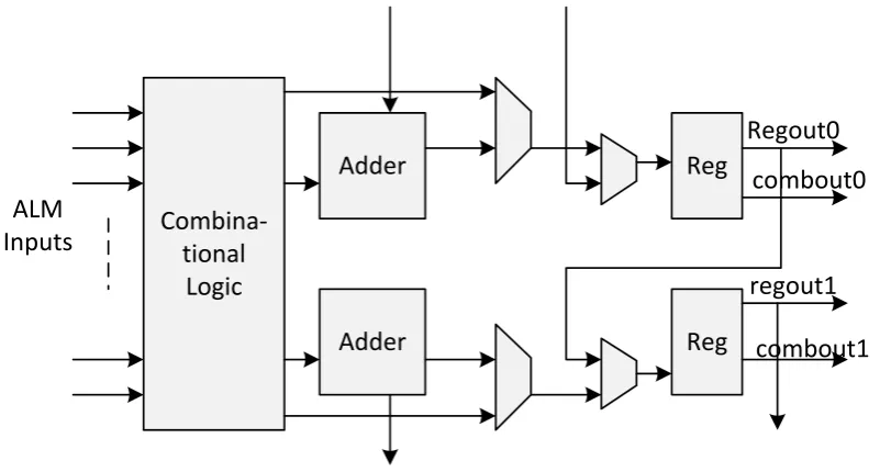
The key to the high-performance, area-efficient architecture is the ALM. It con-sists of combinational logic, two registers, and two adders as shown in Fig. 2.4. The combinational portion has eight inputs and includes a LUT that can be divided between two adaptive LUTs (ALUTs) using Alteras patented LUT tech-nology. An entire ALM is needed to implement an arbitrary six-input function, but because it has eight inputs to the combinational logic block, one ALM can implement various combinations of two functions. A LUT is typically built out of SRAM bits to hold the configuration memory (CRAM) LUT-mask and a set of multiplexers to select the bit of CRAM that is to drive the output. To implement at-input LUT; a LUT that can implement any function oft inputs2tSRAM bits and a 2t: 1 multiplexer are needed.
2.5 Field Programmable Gate Array Architecture 27
Combina-tional
Logic
Adder
Adder
Reg
Reg ALM
Inputs
Regout0
combout1 regout1
[image:47.595.121.522.74.289.2]combout0
Figure 2.4: Internal structure of an ALM.
2D and 3D MRI Processing
Using CS-Based Complex
Measurements
3.1
Introduction
In recent times, compressive sensing (CS) has proved its potential to reduce data acquisition time for magnetic resonance images (MRI). For a CS-based MRI imag-ing scheme to be effective, the signal of interest should be sparse or compressible in a known representation, and the measurement scheme should have good math-ematical properties with respect to this representation. Although the Fourier transform has been commonly used for MRI data, it does not strongly satisfy CS mathematical properties. This limits the achievable time reduction factors necessary for 3D-MRI.
3.2 Related Work 29
Based on compressive sensing methods, the attempt is to provide the following contributions for 2D and 3D MRI:
• Non-Fourier based MRI data acquisition using the complex Hadamard ma-trix and show that, when used with Daubechies-4 wavelet transform satisfies the RIP. This complex Hadamard matrix structure is proposed and used for the first time;
• Complex measurements based CoSaMP reconstruction, whose computa-tional complexity is less than the original CoSaMP;
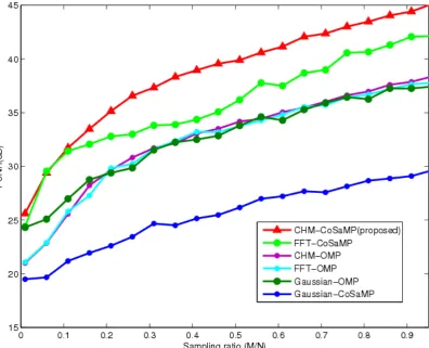
• Comparison of our proposed method with the conventional Fourier sampling and also its efficiency with respect to computational complexity. Further-more, we demonstrate our proposed method through the measure of peak signal-to-noise ratio (PSNR) and compare with the commonly used orthog-onal matching pursuit (OMP) [99] algorithm; and
• Compare results with the NFCS-3D Fista [2] method, and show that our proposed method has higher PSNR for a 3D phantom, when implemented on similar lines as outlined in [2].
3.2
Related Work
Conventional MRI based processing relies on the Fourier transform for data acqui-sition, including 3D and dynamic MRI [2,87–90]. In many instances, it is observed that the Fourier matrices are not necessarily well suited for CS reconstruction for arbitrary sparse matrix Ψ [97]. Since Fourier encoding is not universal, the in-coherent condition is only weakly satisfied with respect to sparse transforms. Some research also suggests that, by using additional slice-selective excitation in a wavelet basis, it is possible to improve 3D image CS reconstruction [3]. For example, a wavelet transform in a coarse scale has its energy concentrated rather than spread out in the Fourier domain, which suggests the incoherence condition is barely satisfied [57]. This shows that the use of matrices other than the Fourier ones could possibly lead to better results.
Hadamard were also proposed [103]
![Figure 5.4: Reconstructed images of a two slices ((a) and (d)) from a total MRIscan samples of dataset-1 [1].](https://thumb-us.123doks.com/thumbv2/123dok_us/151912.29056/89.595.135.510.72.363/figure-reconstructed-images-slices-total-mriscan-samples-dataset.webp)