995
THE SIMULATION OF BIOGAS COMBUSTION IN A MILD BURNER
M. M. Noor1,3, Andrew P. Wandel1 and Talal Yusaf2
1
Computational Engineering and Science Research Centre, School of Mechanical and Electrical Engineering, University of Southern Queensland (USQ), Australia
2
National Center for Engineering in Agriculture, USQ, Australia 3
Faculty of Mechanical Engineering, University of Malaysia Pahang, Malaysia Email: [email protected]
ABSTRACT
This paper discusses the design and development of moderate and intense low oxygen dilution (MILD) combustion burners, including details of the computational fluid dynamics process, step-by-step from designing the model until post-processing. A 40 mm diameter bluff-body burner was used as the flame stabilizer. The fuel nozzle was placed in the center with a diameter of 1mm and an annular air nozzle with an opening size of 1,570 mm2, and four EGR pipes were used. Non-premixed combustion with a turbulent realizable k-epsilon was used in the simulation. The fuel used is low calorific value gas (biogas).The synthetic biogas was a mixture of 60% methane and 40% carbon dioxide. The simulation was successfully achieved during the MILD regime where the ratio of maximum-to-average temperature was less than the required 23%.
Keywords: Combustion; computational fluid dynamics; bluff-body; low calorific value
gas; MILD burner; biogas.
INTRODUCTION
996
has been successful in carrying out simulations of many engineering problems (Baukal Jr, Gershtein, & Li, 2000; Davidson, 2002),such as those for gas turbines (Duwig, Stankovic, Fuchs, Li, & Gutmark, 2007), industrial furnaces (Chen, Yong, & Ghoniem, 2012), boilers (Rahimi, Khoshhal, & Shariati, 2006), internal combustion engines (Devi, Saxena, Walter, Record, & Rajendran, 2004), MILD or flameless combustors (Acon, Sala, & Blanco, 2007; Hasegawa, Mochida, & Gupta, 2002; Noor, M. M., Wandel, A. P., & Yusaf, T., 2013b; Veríssimo, Rocha, & Costa, 2013) and other engineering applications (Fletcher, Haynes, Christo, & Joseph, 2000; Najiha, Rahman, Kamal, Yusoff, & Kadirgama, 2012; Ramasamy et al., 2009; Wandel, Smith, & Klimenko, 2003). Simulations can also be run using discretization of fluid flow equations through the finite difference method (FDM) and Taylor expansion, then writing the coding using FORTRAN (Noor, Hairuddin, Wandel, & Yusaf, 2012; Press, Teukolsky, Vetterling, & Flannery, 1992) or MATLAB (Hairuddin, Yusaf, & Wandel, 2011; Wandel, 2011, 2012). The purpose of this study is to design and develop a model for the MILD combustion burner. This paper drafts, step by step, a CFD simulation for the non-premixed MILD combustion furnace with biogas as a fuel. In addition to experimental testing, computational work is now becoming more and more important due to its lower cost and acceptable accuracy with minimum error. Especially in newly developed models, computational testing using CFD software will reduce much trial and error in experimental work.
CFD GOVERNING EQUATIONS
The governing equations for the CFD calculations are the fluid flow and turbulence governing equations. The equations involve a series of fluid properties; mass conservation (continuity equation), density, temperature, species, mass fraction, enthalpy, turbulent kinetic energy (k) and turbulent dissipation rate (ε). For the axisymmetric flow in low Mach number (M<0.3) (Majda & Sethian, 1985; Rehm & Baum, 1978), the transport equations are:
Mass (the continuity equation)
(1)
Momentum
(2)
Enthalpy
∑ (3)
Temperature
∑ ∑ (4)
Species mass fraction
(5)
997
simple to implement and easy to converge. The equation for turbulent kinetic energy (k) is Equation (6) and turbulent dissipation rate (ε) is Equation (7).
[
] (6)
[
] (7)
where turbulent viscosity, , production of k, , and effect
of buoyancy, and . In the effect of buoyancy is the
component of the gravitational vector in the ith direction and Pr is turbulent Prandtl number. Pr is 0.85 for the standard and realizable k- ε model. Other model constants are
and . The common fluid flow problems can be solved in one, two
or three dimensions with parabolic, elliptic or hyperbolic equations.
MODEL DEVELOPMENT
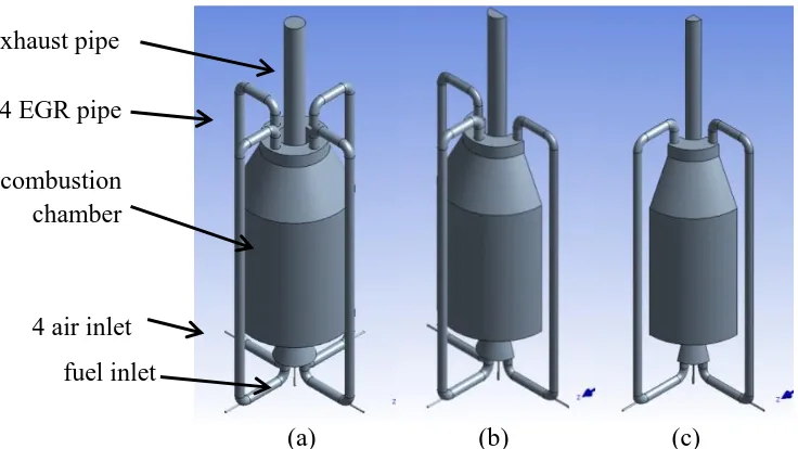
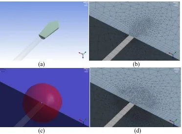
The modeling simulation was designed and developed using ANSYS design modeler software as in Figure 1. In order to expedite the solution, the model must be small and simple, but meet the required model drawing and shape, because the smaller the model, the fewer meshing nodes and elements to be calculated later. The mesh grid quantity will directly impact the solution duration. If the model is symmetrical, it can be halved (Figure1(b)) or even quartered (Figure1(c)). The geometry of the model includes volumes, surface, edges and vertices. All of these items can be taken into account in meshing techniques.
[image:3.595.91.459.492.699.2](a) (b) (c)
Figure 1: MILD furnace (a) the model schematic diagram with boundary condition, (b) half model axisymmetric at xy-plane, (c) quarter model axisymmetric at xy-plane and
yz-plane combustion
chamber exhaust pipe
4 air inlet 4 EGR pipe
998
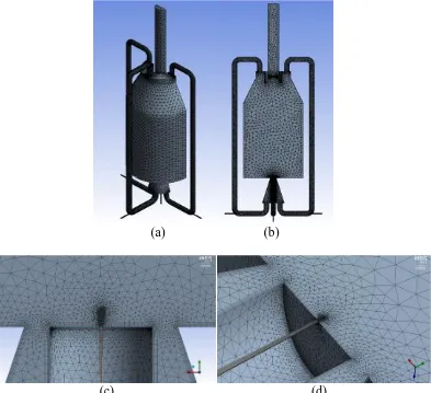
MODEL MESHING
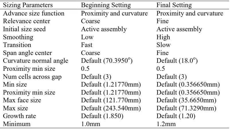
[image:4.595.98.506.525.750.2]The model meshing is the most important and sensitive process in CFD simulations. The quality of meshing will be determined by the technique of the meshing. Meshing will create a grid of cells or elements which are required to solve all the desired fluid flow equations. The size of the grid will give significant impact on the computational time which has direct impact on the cost of simulations. The grid will also have a significant effect on the convergence speed and solution accuracy. Industrial CFD problems normally consist of large numerical grid cells (Peters, 2004). In the meshing process, inflation must be applied for the area near the wall or near the boundary layer mesh. Figures 2(a) and 2(b) show the plain meshing without inflation and detail sizing of some important areas. Figures 2(c) and 2(d) show the meshing with inflation and the nozzle area with the body of influence and edge sizing technique. The meshing process is highly complex and much practice, trial and error is required for its skilled use. Practice can be gained following the ANSYS meshing tutorial available on their website. The meshing process must be start with coarse mesh (Table 1),using statistics to check the quality (Table 2). The required quality check is of the skewness and aspect ratio on mesh metrics and smoothness (changes in cell size). The maximum skewness must be below 0.98 or the solution will easily become a divergence error and will not converge as desired (Noor, M., Wandel, A. P., & Yusaf, T., 2013). Some models and settings may have different limit ranges, from 0.85 to 0.98. The overall range of skewness is from zero to one, where the best is zero and worst is one. The skewness value is calculated based on equilateral or equiangular shape. For example the skewness for equilateral is the ratio of the optimal cell size minus the actual cell size divided by the optimal cell. In this case, coarse mesh gives a maximum skewness of 0.9817,which is higher than the allowable value. A medium or fine mesh is needed to ensure the skewness is below 0.98. When the meshing uses a fine relevance center and other setting as final setting in Table 1, the maximum skewness is lowered to 0.8458,and is below the most rigid limit of 0.85.
Table 1.Mesh sizing setting parameters
Sizing Parameters Beginning Setting Final Setting
Advance size function Proximity and curvature Proximity and curvature
Relevance center Coarse Fine
Initial size seed Active assembly Active assembly
Smoothing Low High
Transition Fast Slow
Span angle center Coarse Fine
Curvature normal angle Default (70.3950o) Default (18.0o)
Proximity min size 0.5 0.5
Num cells across gap Default (3) Default (3)
Min size Default (1.21770mm) Default (0.356650mm)
Proximity min size Default (1.21770mm) Default (0.356650mm)
Max face size Default (121.770mm) Default (35.6650mm)
Max size Default (243.540mm) Default (71.3290mm)
Growth rate Default (1.850) Default (1.20)
999
The aspect ratio is calculated by dividing the longest edge length by the shortest edge. An aspect ratio of 1.0 is the best and means that the cell is nicely square or has equal edge lengths of any shape. The cell shapes were triangular and quadrilateral for the 2D problem and tetrahedron, hexahedron, pyramid wedges and polyhedrons for the 3D problem. The smoothness or the change in cell size must be gradual and must not be more than 20% change from one cell to the next. If there are cells that jump in size, the smoothness will be very bad and the solution will be hard to converge. The node and element quantity is critical since it will affect the final result and the computational time, which involves computational cost. A higher meshing element will give a better final result, but takes longer computational time to complete the simulation. At this point, the acceptable mesh quality will be the best solution for both an acceptable final result and computational time. The dynamic mesh is not applicable to this problem.
(a) (b)
[image:5.595.103.496.264.623.2](c) (d)
Figure 2.The model meshing with course mesh in the middle and fine mesh at critical locations, such as near walls or air and fuel nozzles (a) full meshing 3D view, (b) 2D
view for meshing, (c) 2D view for fine mesh using body of influence at fuel and air nozzle inlet, (d) 3D view for fine mesh at fuel and air nozzle inlet
1000
[image:6.595.107.490.249.432.2]jets mixes with the air jet, a super fine mesh is needed, and this can be provided by using the body sizing meshing technique. There are 3 types of body sizing: element size, sphere of influence and body of influence. For the body of influence, the scope geometry is the whole body selection and a frozen body needs to be added and drawn in the design model as in Figure 3(a). The mesh result for the body of influence, shown in Figure 3(b),is very sensitive and the process needs to be repeated until it is stable (repeat by removing the frozen body, drawing again). The sphere of influence will give a higher number of nodes and elements. The sphere center and radius need to be selected, normally using the xy-plane as in Figure 3(c). The mesh result is shown in Figure 3(d).
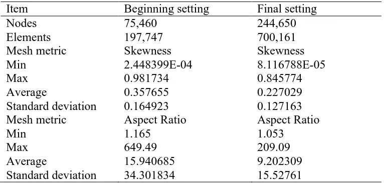
Table 2.Statistics on nodes, elements and mesh metrics for skewness and aspect ratio.
Item Beginning setting Final setting
Nodes 75,460 244,650
Elements 197,747 700,161
Mesh metric Skewness Skewness
Min 2.448399E-04 8.116788E-05
Max 0.981734 0.845774
Average 0.357655 0.227029
Standard deviation 0.164923 0.127163
Mesh metric Aspect Ratio Aspect Ratio
Min 1.165 1.053
Max 649.49 209.09
Average 15.940685 9.202309
[image:6.595.163.434.472.697.2]Standard deviation 34.301834 15.52761
Table 3.The parameter settings for inflation.
Item Setting
Use automatic inflation Program controlled
Inflation option Total thickness
Inflation algorithm Pre
View advanced option Yes
Collision avoidance Stair stepping
Growth rate type Geometric
Use post smoothing Yes
Number of layers 5
Growth rate 1.2
Maximum thickness 2.mm
Gap factory 0.5
Maximum height over base 1
Maximum angle 140.0
Fillet ratio 1
1001
(a) (b)
[image:7.595.113.485.82.356.2](c) (d)
Figure 3. Body sizing mesh for (a) geometry of body of influence, (b) meshing of body of influence, (c) geometry of sphere of influence, (d) meshing of sphere of influence
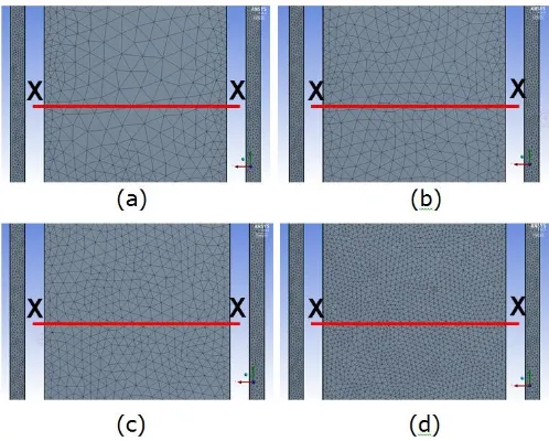
In order to simulate and access the high accuracy of the modeling, and to ensure that mesh independence is applies, a grid independence study was performed for different mesh settings. Grids A, B, C and D were generated to simulate the temperature profile in the combustion chamber. The maximum skewness was 0.873, 0.898, 0.882 and 0.888 for grid A, B, C and D respectively, which is below the allowable limit of 0.98. Maximum skewness must be below 0.98 or the solution will easily become a divergence error and will not converge as desired. Temperature distribution was measured in the middle of the chamber and the result is as depicted in Figure4. Figure 4(a) - (d) show the different grid sizes of grids A, B C and D. The cross-section of the chamber marked as X-X axis is generated in the model in Figure4 to compare the temperature reading in this axis. As a result, Grids C and D give almost identical results as shown in Figure5.
1002
Figure 4. Meshing independence (a) mesh grid A,(b) mesh grid B,(c) mesh grid C,(d) mesh grid D.
MODELLING SOLUTION SETUP
Single or double precision must be set as an option during solution setup If double precision is used, the solution will be slower, and this is not necessary for many cases. The processing option involves the setting of a single or parallel processor on a local machine. A maximum of four parallel computer processors can be used with one license. This is applicable to multicore processor computers, but not single processor computers. To increase the parallel processor to more than four, a second license is needed. The steps are as follows:
1003
[image:9.595.168.428.118.317.2]the normal combustion air configuration. The fuel and oxidant temperature was set at 300K.
[image:9.595.176.419.380.447.2]Figure 5.Temperature distribution for X-X axis for grid A, B, C and D.
Table 4. PDF table creation for boundary condition parameters.
Species Fuel Oxidant CH4 0.60 0
N2 0 0.79 O2 0 0.21 CO2 0.40 0
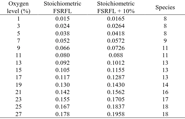
PDF mixture is used for the material and the species count is dependent on the model setting (Table 5). The pressure is set at 101.325kPa and the fuel stream rich flammability limit is set as Table 5 for model setting under the setting for non-premixed combustion.
Table 5. PDF table creation for model setting parameters for fuel stream rich flammability limit (FSRFL).
Oxygen level (%)
Stoichiometric FSRFL
Stoichiometric
[image:9.595.138.457.563.768.2]1004
After this setting is confirmed, set the inlet diffusion at the PDF option with automated grid refinement. The next step is to calculate PDF table and display the results. The PDF table can be checked by displaying the PDF table, choosing the figure type as 2D or 3D, and which parameters to display (the default is the 3D figure: mean temperature, mean mixture fraction and scaled variance). The boundary condition is the setting for the inlet, wall and outlet. In this case there are four air inlets, one fuel inlet, one exhaust and one wall for the whole chamber. For the air inlet and fuel inlet, the momentum setting for the velocity specification method uses the component method. The Cartesian coordinate system was used in line with the model coordinate system. The velocity for the air inlet was in the x and z direction. Under the thermal setting, the temperature was set to 300K and for the species setting; the mean mixture fraction was set to zero. The velocity for the fuel inlet was in Y direction and thermal (temperature) setting was 300K, but the mean mixture fraction was set to unity. The turbulence specification method was ‘intensity’ the hydraulic diameter which involves turbulence intensity was set to 5% and the hydraulic diameter to10mm as per model measurement. The velocity for the air and fuel inlet, in unit m/s, is one of the main parameters to change, depending on the air fuel ratio of the biogas and oxidant (Noor, Wandel, et al., 2012). The wall setting is ‘stationary wall’ and ‘no slip shear’ condition with thermal heat flux 0 w/m2 and an internal emissivity of one.
MODELLING SOLUTION
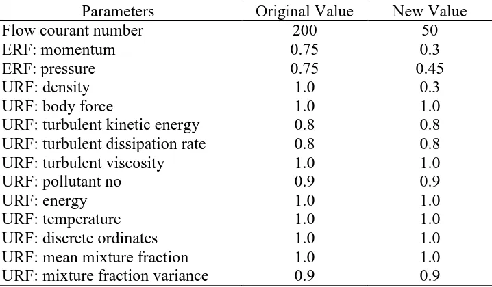
The solution of the simulation involves chemical reactions since it is a non-premixed combustion process, involving heat transfer, turbulent flows and species transport. The simulation used Reynolds-Averaged Navier–Stokes (Lindberg, Hörlin, & Göransson) equations solved together with a realizable k-ε turbulence model (Shih, Liou, Shabbir, Yang, & Zhu, 1995) [that was developed based on the standard k-ε turbulence model (Launder & Spalding, 1974)] solved using commercial CFD software ANSYS Fluent 14.5 (Fluent Inc, 2012). The discrete ordinate (DO) radiation model (Chui & Raithby, 1993; Fiveland, 1984) and absorption coefficient of the weighted sum of gray gas (WSGGM) model (Hottel & Sarofim, 1967; Smith, Shen, & Friedman, 1982; Soufiani & Djavdan, 1994) was used in this work. The selection of the WSGGM model is suitable for this work as it gives a reasonable compromise between oversimplified gray gas assumption and the complete model, accounting for the entire spectral variation of radiation properties (Yeoh & Yuen, 2009). The solution method setting (Table6) shows the original and new settings for the case. The couple method is used for the pressure-velocity coupling scheme with least square cell based gradient and presto for pressure. The second order upwind is suitable for the momentum, turbulent kinetic energy, turbulent dissipation rate, pollutant no, energy, discrete ordinates, mean mixture fraction, and mixture fraction variance, when the solution is run in the final stage.
1005
[image:11.595.89.504.149.318.2]pressure and density as shown in Table 7. The reduction of the relaxation factor will slow the convergence process.
Table 6.The parameter setting for the solution method.
Parameters Original Setting New Setting
Pressure-velocity coupling Simple Couple
Gradient Green-gauss cell based Least squares cell based
Pressure standard PRESTO!
Momentum First order upwind Second order upwind
Turbulent kinetic energy First order upwind Second order upwind
Turbulent dissipation rate First order upwind Second order upwind
Pollutant no First order upwind Second order upwind
Energy First order upwind Second order upwind
Discrete ordinates First order upwind Second order upwind
Mean mixture fraction First order upwind Second order upwind
Mixture fraction variance First order upwind Second order upwind
Table 7.Solution control parameters for flow Courant number, explicit relaxation factor and under-relaxation factor.
Parameters Original Value New Value
Flow courant number 200 50
ERF: momentum 0.75 0.3
ERF: pressure 0.75 0.45
URF: density 1.0 0.3
URF: body force 1.0 1.0
URF: turbulent kinetic energy 0.8 0.8
URF: turbulent dissipation rate 0.8 0.8
URF: turbulent viscosity 1.0 1.0
URF: pollutant no 0.9 0.9
URF: energy 1.0 1.0
URF: temperature 1.0 1.0
URF: discrete ordinates 1.0 1.0
URF: mean mixture fraction 1.0 1.0
URF: mixture fraction variance 0.9 0.9
[image:11.595.120.479.372.582.2]1006
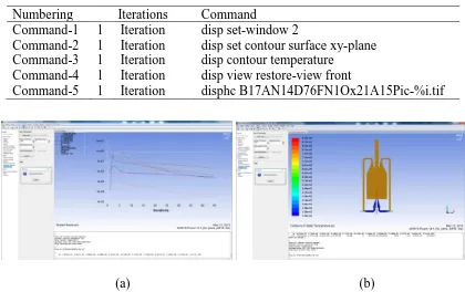
[image:12.595.87.507.190.454.2]individualliteration. The iteration pictures that are generated by that command will be saved as running numbers with 0001 to 9999 at the end of the filename (B17AN14D76FN10x21A15Pic-0001.tif). The display during the calculation will be shown as Figure 6, where residual monitoring is in Window 1 (Figure 6(a)) and the xy-plane contour surface in Window 2 (Figure 6(b)).
Table 8. Execute commands under calculation activities.
Numbering Iterations Command
Command-1 1 Iteration disp set-window 2
Command-2 1 Iteration disp set contour surface xy-plane
Command-3 1 Iteration disp contour temperature
Command-4 1 Iteration disp view restore-view front
Command-5 1 Iteration disphc B17AN14D76FN1Ox21A15Pic-%i.tif
(a) (b)
Figure 6. Monitoring window during calculation (a) Window 1, (b) Window 2
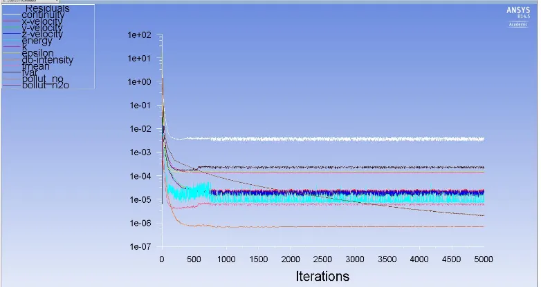
Before the calculation process starts, a case check needs to be made to ensure that there are no errors and that the model is ready to be simulated. The check case checks the mesh, models, boundaries and cell zone, materials and solver. In this example, the calculation was set up at 4500 iterations, as in Figure 7. The calculation was converging and the result was satisfied when non-premixed combustion occurred and MILD achieved as expected. There was much trial and error to achieve the convergence, especially of the explicit relaxation factor (ERF) and under-relaxation factor (Alfriend et al.). Figure 8 shows one of the examples of common error which is a primitive error at Node 1: a floating point exception (divergence detected in AMG solver: enthalpy or some time the error of divergence detected in AMG solver: epsilon). To solve this error flow, the Courant number and three relaxation factor is tested and finally reaches the optimum values.
The convergence of the solution is very important to ensure that the end result of the simulation is correct and accurate. The relaxation method may be used to accelerate or delay the solution, using the relaxation factor. The relaxation factor (λ) can be seen in the equation below,
1007
[image:13.595.103.494.186.394.2]where λ is between 1-2 and is the value from the present iteration and is the value from the past iteration. The convergence can be monitored by the residual (Figure 7 and 8). If λ is less than 1.0 this is under-relaxation and will slow down the convergence and the simulation will take longer. Under-relaxation will increase the calculation stability and reduce the divergence possibility. If λ is equal to 1.0, it means there is no relaxation applied. If λ is more than 1.0 it is over-relaxation.
Figure 7. Converge solution
Over-relaxation will accelerate the convergence but at the same time will reduce the calculation stability and give a high probability of the solution diverging. The most sensitive relaxation factors in the combustion simulation are energy, temperature, radiation (discrete ordinates) and mean mixture fraction. These items will normally use 1.0 as relaxation factors. For an under-relaxation factor (Table 7), it is advice is to use a high relaxation factor (near to or 1.0) since if it too low, the convergence will be too slow and may not be converged, even if it appears to converge. The default relaxation factor is the factor proposed by the solver and if the solution is still diverged, the explicit relaxation factor (momentum and pressure) can be reduced to slow convergence (Table 7).
MODELLING RESULTS
1008
[image:14.595.85.512.172.378.2]convergence of the simulation is considered achieved if the residual is stable or there is no more change from one iteration to the next iteration (Figure 7). If the residual has already achieved the lower limit set by the residual monitor but is still showing a reducing trend, the solution may not be converged until the residual is stable. The lower limit for the residual is normally set at 1.0 x 10⁻⁶. In some cases the lower limit is set at between 1.0 x 10⁻³ to 1.0 x 10⁻⁶.
[image:14.595.165.431.450.535.2]Figure 8.Error on divergence detected in AMG solver: enthalpy
Table 9. Point for 2D xy-plane setting the view contour result
x0 x1 x2
-486mm -486mm 486mm
y0 y1 y2
-438mm -438mm 1750
z0 z1 z2
0 0 0
1009
preheating and dilution of the oxidant causes the furnace to achieve a MILD combustion regime.
[image:15.595.143.452.136.363.2](a) (b)
Figure 9.The contour result for (a) 2D view for velocity magnitude (unit: m/s), (b) 3D view for temperature distribution (units: Kelvin).
(a) (b) (c)
[image:15.595.88.510.416.687.2]1010
CONCLUSIONS
The CFD simulation was completed and in summary, below conclusions can be drawn from the simulation of non-premixed MILD combustion.
i. The most important and critical step in CFD work is meshing. The quality of meshing has the highest influence on whether the calculations will converge and produce good results or diverge and give an erroneous result.
ii. The meshing quality can be checked by the skewness, aspect ratio on mesh metrics and smoothness. The maximum skewness must not exceed 0.98.
iii. The selection of the solution method and solution control must be suitable for the model and equation to be solved.
iv. Divergence of the solution can commonly be solved by changing the explicit under relaxation factors. The advisable changing rate is about 10% for each new simulation.
v. Residual monitoring is a very useful tool to monitor the iteration steps and whether they converge or diverge. The residual will be converged when the value is stable and not decreasing.
vi. The fresh air was preheated by the EGR from 300K to the range of 418 to 537K,and the oxygen was diluted, resulting in the burner achieving MILD combustion conditions as expected.
vii. The simulation successfully achieved the objectives of the MILD regime where the ratio of maximum-to-average temperature was less than the required 23% for MILD conditions.
ACKNOWLEDGMENTS
The authors would like to thank the University of Southern Queensland (USQ), Ministry of Higher Education, Malaysia (MOHE) and Universiti Malaysia Pahang (Bumpus) for providing financial support and laboratory facilities.
REFERENCES
Acon, C., Sala, J., & Blanco, J. (2007). Investigation on the design and optimization of a low nox-co emission burner both experimentally and through cfd simulations. Energy and Fuels, 21(1), 42-58.
Alfriend, K., Vadali, S. R., Gurfil, P., How, J., & Breger, L. (2010). Spacecraft formation flying: Dynamics, control, and navigation (Vol. 2): Butterworth-Heinemann.
Arghode, V. K., & Gupta, A. K. (2011). Development of high intensity cdc combustor for gas turbine engines. Applied Energy, 88(3), 963-973.
Baukal Jr, C. E., Gershtein, V., & Li, X. J. (2000). Computational fluid dynamics in industrial combustion. New York: CRC press.
Bumpus, S. R. J. (2002). Experimental setup and testing of fiber reinforced composite structures. (Master), University of Victoria.
1011
Chen, L., Yong, S. Z., & Ghoniem, A. F. (2012). Oxy-fuel combustion of pulverized coal: Characterization, fundamentals, stabilization and cfd modeling. Progress in Energy and Combustion Science, 38(2), 156-214.
Chen, Q.-S., Wegrzyn, J., & Prasad, V. (2004). Analysis of temperature and pressure changes in liquefied natural gas (lng) cryogenic tanks. Cryogenics, 44(10), 701-709.
Chui, E., & Raithby, G. (1993). Computation of radiant heat transfer on a nonorthogonal mesh using the finite-volume method. Numerical Heat Transfer, 23(3), 269-288.
Colorado, A., Herrera, B., & Amell, A. (2010). Performance of a flameless combustion furnace using biogas and natural gas. Bioresource Technology, 101(7), 2443-2449.
ally . . him . . raig . . shman . J. eg . . (2010). On the burning of sawdust in a mild combustion furnace. Energy & Fuels, 24(6), 3462-3470.
Davidson, D. L. (2002). The role of computational fluid dynamics in process industries. The Bridge, 32(4), 9-14.
Devi, R., Saxena, P., Walter, B., Record, B., & Rajendran, V. (2004). Pressure reduction in intake system of a turbocharged-inter cooled di diesel engine using cfd methodology: SAE Technical Paper.
Duwig, C., Stankovic, D., Fuchs, L., Li, G., & Gutmark, E. (2007). Experimental and numerical study of flameless combustion in a model gas turbine combustor. Combustion Science and Technology, 180(2), 279-295.
Fiveland, W. (1984). Discrete-ordinates solutions of the radiative transport equation for rectangular enclosures. Journal of Heat Transfer, 106(4), 699-706.
Fletcher, D., Haynes, B., Christo, F., & Joseph, S. (2000). A cfd based combustion model of an entrained flow biomass gasifier. Applied Mathematical Modelling, 24(3), 165-182.
Fluent Inc. (2012). Fluent 14.5 user's guide.
Hairuddin, A. A., Yusaf, T. F., & Wandel, A. P. (2011). Predicting the combustion behaviour of a diesel hcci engine using a zero-dimensional single-zone model. Paper presented at the Proceedings of the Australian Combustion Symposium 2011, Newcastle, Australia.
Hasegawa, T., Mochida, S., & Gupta, A. (2002). Development of advanced industrial furnace using highly preheated combustion air. Journal of propulsion and power, 18(2), 233-239.
Hottel, H. C., & Sarofim, A. F. (1967). Radiative transfer. New York: McGraw Hill. IEA. (2009). World energy outlook. Paris: International Energy Agency.
Jones, W., & Launder, B. (1972). The prediction of laminarization with a two-equation model of turbulence. International Journal of Heat and Mass Transfer, 15(2), 301-314.
Katsuki, M., & Hasegawa, T. (1998). The science and technology of combustion in highly preheated air. Symposium (International) on combustion, 27(2), 3135-3146.
Keramiotis, C., & Founti, M. A. (2013). An experimental investigation of stability and operation of a biogas fueled porous burner. Fuel, 103, 278-284.
1012
Launder, B., & Sharma, B. (1974). Application of the energy-dissipation model of turbulence to the calculation of flow near a spinning disc. Letters in heat and mass transfer, 1(2), 131-137.
Launder, B. E., & Spalding, D. (1974). The numerical computation of turbulent flows. Computer Methods in Applied Mechanics and Engineering, 3(2), 269-289. Li, P., Mi, J., Dally, B. B., Wang, F., Wang, L., Liu, Z.et al.Zheng, C. (2011). Progress
and recent trend in mild combustion. Science China Technological Sciences, 54(2), 255-269.
Lindberg, E., Hörlin, N.-E., & Göransson, P. (2013). An experimental study of interior vehicle roughness noise from disc brake systems. Applied Acoustics, 74(3), 396-406.
Maczulak, A. (2010). Renewable energy: Sources and methods. New York: Facts on File Inc.
Majda, A., & Sethian, J. (1985). The derivation and numerical solution of the equations for zero mach number combustion. Combustion Science and Technology, 42(3-4), 185-205.
Najiha, M. A., Rahman, M. M., Kamal, M., Yusoff, A. R., & Kadirgama, K. (2012). Mql flow analysis in end milling processes: A computational fluid dynamics approach. Journal of Mechanical Engineering and Sciences, 3, 340-345.
Noor, M., Hairuddin, A. A., Wandel, A. P., & Yusaf, T. (2012). Modelling of non-premixed turbulent combustion of hydrogen using conditional moment closure method. IOP Conference Series: Materials Science and Engineering, 36, 1-17. Noor, M., Wandel, A. P., & Yusaf, T. (2012). A review of mild combustion and open
furnace design consideration. International Journal of Automotive and Mechanical Engineering, 6(1), 730-754.
Noor, M., Wandel, A. P., & Yusaf, T. (2013). The analysis of recirculation zone and ignition position of non-premixed bluff-body for biogas mild combustion. Paper presented at the Proceedings of the 2nd International Conference of Mechanical Engineering Research, Malaysia.
Noor, M. M., Wandel, A. P., & Yusaf, T. (2013a). Analysis of recirculation zone and ignition position of non-premixed bluff-body for biogas mild combustion. International Journal of Automotive and Mechanical Engineering, 8, 1176-1186.
Noor, M. M., Wandel, A. P., & Yusaf, T. (2013b). Design and development of mild combustion burner. Journal of Mechanical Engineering and Sciences, 5, 662-676.
Peters, N. (2004). Turbulent combustion. UK: Cambridge University Press.
Press, W. H., Teukolsky, S. A., Vetterling, W. T., & Flannery, B. P. (1992). Numerical recipes in fortran. UK: Cambridge University Press.
Rahimi, M., Khoshhal, A., & Shariati, S. M. (2006). Cfd modelling of a boilerstubes rupture. Applied Thermal Engineering, 26, 2192-2200.
Ramasamy, D., Noor, M. M., Kadirgama, K., Mahendran, S., Redzuan, A., Sharifian, S. A., & Buttsworth, D. R. (2009). Validation of drag estimation on a vehicle body using cfd. Paper presented at the Europe Power and Energy Systems, Spain. Rehm, R., & Baum, H. (1978). The equation of motion for thermally driven bouyant
flows. N. B. S. J. Res, 83, 297-308.
1013
Shafiee, S., & Topal, E. (2009). When will fossil fuel reserves be diminished? Energy Policy, 37(1), 181-189.
Shih, T.-H., Liou, W. W., Shabbir, A., Yang, Z., & Zhu, J. (1995). A new k-ϵ eddy viscosity model for high reynolds number turbulent flows. Computers & Fluids, 24(3), 227-238.
Smith, T., Shen, Z., & Friedman, J. (1982). Evaluation of coefficients for the weighted sum of gray gases model. Journal of Heat Transfer, 104(4), 602-608.
Soufiani, A., & Djavdan, E. (1994). A comparison between weighted sum of gray gases and statistical narrow-band radiation models for combustion applications. Combustion and Flame, 97(2), 240-250.
Tsuji, H., Gupta, A., Hasegawa, T., Katsuki, M., Kishimoto, K., & Morita, M. (2003). High temperature air combustion, from energy conservation to pollution reduction. Boca Raton,FL: CRC Press.
Veríssimo, A., Rocha, A., & Costa, M. (2013). Importance of the inlet air velocity on the establishment of flameless combustion in a laboratory combustor. Experimental Thermal and Fluid Science, 44, 75-81.
Wandel, A. P. (2011). A stochastic micro mixing model based on the turbulent diffusion length scale. Paper presented at the Australia Combustion Symposium, Newcastle, Australia.
Wandel, A. P. (2012). Extinction precursors in turbulent sprays. Paper presented at the International Symposium on Combustion, Poland.
Wandel, A. P., Smith, N. S., & Klimenko, A. (2003). Implementation of multiple mapping conditioning for single conserved scalar Computational fluid dynamics 2002 (pp. 789-790): Springer.
Wünning, J. (1991). Flammenlose oxidation von brennstoffmithochvorgewärmterluft. ChemieIngenieurTechnik, 63(12), 1243-1245.
Yeoh, G. H., & Yuen, K. K. (2009). Computational fluid dynamics in fire engineering: Theory, modelling and practice: Butterworth-Heinemann.