An experimental investigation of the turbulent boundary layer over a wavy wall

(1)

TURBULENT BOUNDARY LAYER OVER A WAVY WALL

Thesis by Asher Sigal

In Partial Fulfillment of the Requirernents For the Degree of

Doctor of Philosophy

California Institute of Technology Pasadena, California

1971

(2)

ACKNOWLEDGMENTS

It is a most pleasant duty for me to express my sincere appreciation and thanks to Professors Lester Lees and Toshi Kubota for their joint guidance. As teachers and advisors, their interest, encouragement and invaluable advice accompanied me throughout the course of my graduate work in GALCIT.

I would also like to express my gratitude to Dr. James Kendall from J. P. L. for ITlaking his laboratory available to ITle and for his help, advice and stim.ulating discussions.

I wish to acknowledge the receipt of financial support from the California Institute of Technology (1967-1971). The work discussed in this thesis was carried out under the sponsorship and with the financial support of the U. S. A. F. Space and Missile Systems Organi-zation, Contract No. F04701-68-C-0151.

(3)

ABSTRACT

An experimental investigation of turbulent boundary layer flow over wavy surfaces was conducted at low speed.

Two models with the ratio of the amplitude to the wave length a/A = 0.03 and wave lengths A = 6" and 1211 were tested in an open-circuit wind tunnel. The free stream velocity was 15.4 m/sec, giving Reynolds number Re = 2. 54 X 10 per inch. Boundary-layer thickness 4 varied from 0

=

1.

5" to 0

=

4.111 by means of boundary-layer trips of va rious height, in 0 rde r to chang e the ratio A

/0.

The following measurements were taken:

*

Wall pressure distribution

*

Average velocity and turbulence level, using a single element hot-wire probe

*

Wall stress distribution, using Preston's tube

*

Static and total pres sures

*

Turbulence intensities and shear stress using X-array hot-wire probe.

An appreciable modulation of all the flow quantities, imposed by the wavy boundary. is observed throughout the investigation. Wall pressure is much lower than predicted by uniform, inviscid theory and is slightly non-symmetric. Wall stress distribution has a peak with C/C_f

o

=

1.

2 upstream of the crest and a dip of C/C

f = 0.6 upstream o

(4)

The turbulence intensities and shear stress distributions near the wall show oscillatory modulation superimposed on the reference flat plate profiles. The amplitude of the oscillations decay exponen-tially toward the edge of the layer, so that in the outer part of the layer the turbulence quantities are practically independent of the longitudinal position.

It was found that Coles' Law of the Wall does not apply in the present situation because of the modulation of the slope of the semi-logarithmic portion of the velocity profiles. A presentation of velocity profiles is suggested through the use of total velocity defined by

-2 1..

(u

+

2 (p _p ) / p } 2 •

00 This quantity obeys the Law of the Wake.

(5)

IV. MEASUREMENTS AND RESULTS

IV.1. Wall Pressure

IV. 2. Velocity Profiles and Turbulence Level Effect of Boundary Layer Thickness Development of the Flow

Test for Two -Dimensionality

19

22 23 24

(6)

Part

Table of Contents (Cont'd) Title

IV.3. Wall Stress

Preston Tube Probe Design Method of MeasurelTIent Results

IV.4. Static Pressure Survey Choice of Static Probe

Disc Probe Sphe re Probe Needle Probe Results

IV.5. Total Pressure Survey Probe and MeasurelTIents

Check for Static Pressure Results IV.6. Turbulence MeasurelTIent

X-Array Probes and Their Calibration Stations of Survey

COlTIparison with the Results of a Single ElelTIent Probe

Turbulence Intensities Turbulent Shear Stres s

Mixing Length and Eddy Vis cosity

Page 25 25 28

29

31 32 32 33 33 34 36 36 36 37 37 38

39

40 41

42 V. ANALYSIS OF THE RESULTS

V.I. Boundary Layer Thicknes ses. StrealTIlines

and Shape Factor 45

(7)

Part

V.3.

V.4. V.5.

V.6.

V.7.

Table of Contents (Cont'd) Title

Validity of Ludwig and Tillmann Skin Friction Law

Law of the Wall

Total Pressure and Total Velocity The Wall Layer

Turbulent Shear Models

Mixing Length and Eddy Viscosity Energy Method

Reduction of Mixing Length and Eddy Viscosity to Unified Form

Page

50 51 53

56

59

60

61 VI. SUMMARY AND CONCL USIONS

VI. 1. Effect of the Parameter A/6

VI. 2. The Outer Layer VI. 3. The Wall Layer

VI. 4. Turbulent Shear Models

VI. 5. Suggestions for Further Research FIGURES

APPENDIX A: Calibration and Data Reduction of

64

65

66

X-Array Hot-Wire Probes 162

APPENDIX B: Curvature Effect on Mixing Length 170 APPENDIX C: Inviscid Small Perturbation Analysis

of the Outer Layer 174

APPENDIX D: Analysis of the Wall Layer 184

(8)

LIST OF FIGURES

Number Title

1 Wind Tunnel-General View 2 Experimental Set- Up

3 Wavy Wall Models - Details of Construction 4 Wavy Wall Models

5 Shape of Wavy Wall Models 6 Measurement of Pressures

7 Calibration of Airspeed at the Center of the Test Section

8 Measurement of Boundary Layer Profile and Turbulence Level Using Single Element Hot-Wire Probe

9

Calibration of Single Element Hot Wire Probes 10 Compensation for Boundary Layer Growth 11 Average Velocity and Free Stream Turbulence

in the Test Section

12 Location of the Two Models and the Corresponding Reference Profiles in the Test Section

13 Reference Velocity and Turbulence Level Profiles 14 Reference Profiles Reduced to Similarity

Coordinates 15

16

17

18

Comparison Between Measured Wall Friction Coefficient and Ludwig and Tillmann Friction Law

Surface Pressure Distribution Along Wavy Wall Models (T = 0.5")

Comparison of Surface Pres sure Distribution for All the Cases

Pressure Coefficient Distribution, Average Velocity and Turbulence Level at Four Stations of Survey

Page

68

69

70 71 72

74

75

76

77

78

79

80

81

85

89

90

91

(9)

List of Figures (Cont'd)

NUITlber Title

19 Average Velocity and Turbulence Level Distribution

20 Effect of Boundary Layer Trip Height on Average Velocity and Turbulence Level

21 DevelopITlent of Velocity Profile Along the Wavy Wall Model

22 Test for Two-DiITlensionality of the Flow Over the Wavy Wall

23 Preston Tube Probe 24 Wall Shear Distribution

25 Disc Probe and its Calibration in Free StreaITl 26 Calibration of Disc Probe in the Boundary Layer 27 Sphere Probe and its Calibration in Free StreaITl 28 Calibration of Sphere Probe in the Boundary Layer 29 Needle Probe and its Calibration in Free StreaITl 30 Calibration of Needle Probe in the Boundary Layer 31 Static Pres sure Distribution

32 COITlparison of Direct and Indirect MeasureITlent of Total Pres sure Coefficient

33 Special X -Ar ray Hot Wire Probe

34 MeasureITlent at Turbulent Intensities and Reynolds Stress Using X-Array Hot Wire Probe

35 Velocity COITlponents, Turbulent Intensities and Reynolds Stress Distribution

36 DevelopITlent of Average Velocity Profiles 37 Turbulence Intensities Distribution

38 Turbulent Shea r Stres s Coefficient Distribution

Page

94

100

108

112 116 118 120 121 122 123 124 125 126

128 131

132

(10)

List of Figures (Cont1d)

Number Title

39 Mixing Length Distribution 40 Eddy Viscosity Distribution

41 Height of Streamlines Above Surface and Boundary Layer Thicknesses

42 Comparison Between Measured Skin-Friction and Ludwig and Tillmann Law

43 Modulation of the Slope Factor Along the Wavy Wall

44 Dependence of Total Pressure Upon Streamline 45 Law of the Wake Fitted to Total Velocity Profiles 46 Log-Log Presentation of Velocity and Total

Velocity

47 Comparison Between Measured Shear Stres s Coefficient and Bradshaw and Ferris Model 48 Comparison Between Measured Eddy Viscosity

and Mellor and Harring Model

49 Mixing Length Based on Total Velocity 50 Eddy Viscosity Based on Total Velocity

Al Calibration of X-Probe: Dependence of Output Upon Velocity

A2 Calibration of X -P robe: Dependence of Output Upon Angle

A3 Calibration at X-Probe: Noise Due to Prong Interference

Bl

Cl

Analysis of Curved Channel Mixing Length Distribution Using Sawyer1s Theory

Comparison Between Inviscid Small Perturbation Analysis of the Outer Layer and Measurement

Page 144 146

148

150

151 152 154

156

158

159 160 161

167

168

169

172

(11)

A,B,C,D Al

a C

d

E H H h K

.t s

p

Pm

LIST OF SYMBOLS

calibration constants of X -ar ray hot-wire probe constant in Van Driest damping factor

amplitude of wavy wall

constant in Coles' Law of the Wall (= 5. 0) drag coefficient

T w

li

P V

~,

skin friction coefficient

T

Ii

p

V~,

turbulent shear stress coefficient

2

(p-po)li

p VO' pressure coefficient

Integration constant (Appendix B) Stanton tube dimension

hot-wire probe output voltage height of test section

*

o

I~, form factor

boundary layer compensation height (Sec. II. 6) calibration constant

mixing length

mixing length based on Sawyer's theory

mixing length based on total velocity pressure

1 2

"2 P V 0' dynamic pres sure

probe's measured pressure (Sec. II. 4) Preston probe pressure

(12)

Po

Q

q

R u , V, w u

r

1 1 1

U , V ,w

Vo

Vt u T u+ X X Y Ys Yw y+ Cl'

i3

0

0*

E: E: T1

List of SyITlbols (Cont'd)

reference pressure (ITleasured at STN 5, sidewall port) resultant velocity (Sec. II. 7)

-,2 -/2 -,2

%

(u

+

V

+

w )

radius of curvature velocity cOITlponents

reference velocity (Sec. V. I) turbulent velocity cOITlponents

reference velocity freestreaITl velocity ITleasured at STN 4%)

-2 1.

(V +2(p-p )/p)2, total velocity (Sec. V.4) o

1

(T / P )2, friction velocity w

u/u

T' norITlalized velocity

Mellor-Herring paraITleter (Sec. V.7) coordinate along centers of surface wave distance froITl wavy wall

surface of wavy wall

wall layer thicknes s (Appendix B)

y u

lv,

norITlalized distance froITl the wall

T

2rr/'A.

>.'<

o

dp/dx/T , Clauser's paraITleter w

boundary layer thickness displaceITlent thicknes s eddy vis cosity

2rra/'A.

(13)

1. INTRODUCTION

In the last few years a study was conducted at GALCIT in con-nection with the phenorn.ena of cros s -hatching ablation. This phenorn.-ena is the forrn.ation of diarn.ond shaped waves on surfaces undergoing ablation in flight test and in a variety of ground test facilities, for rn.any types of ablative rn.aterials. The surface waves have character-istic length and sweep angle with respect to the flow direction. At the present tirn.e, the phenorn.ena is not yet corn.pletely unde rstood. In particular, it has not yet been established whether the phenorn.ena is a reflection of a periodic phenorn.ena in the structure of supersonic turbulent boundary layer or a result of unstable interaction between the flow and the ablation process. But, regardless of the initiation of the surface patte rn, it is corn.rn.only agreed that the proces s of the growth of waves has to be considered as a closed loop cycle, i. e., once striation starts the resulting change in surface georn.etry is fed back into the boundary layer, causing significant changes in the dis-tribution of such aerodynarn.ic quantities as pressure, wall stress and heat transfer that are responsible for the forrn.ation of the surface waves.

(14)

Com.putational methods of turbulent boundary layers are usually divided into two groups: integral methods and differential methods. Bc.::ause of the curvature of the streamlines, it is apparent that the velocity profiles commonly used in integral methods (e. g., Coles 1 Law

of the Wake, Power Law) will not properly des cribe the situation. Also, the validity of the friction laws applicable to flat surfaces (e. g. Ludwig and Tillmann)(lO) is in doubt. Therefore, studies performed at GALCIT

*

were devoted to the development of differential computational methods. The differential methods depend on some models that relate Reynolds stres ses to the flow conditions. Thes e cOInInonly us ed

models relate the turbulent stresses either to the mean flow quantities or to the turbulent energy. Common to all the methods is the use of empirical functions and constants. Most of these functions and con-stants were derived from the results of experiments with boundary layers over flat surfaces.

A serious question constantly asked is the validity of these laws: How much can their range of applicability be stretched? More specifically for the present problem: May these laws be used where curvature effects are of importance?

Curvature effect on turbulent boundary laye r was the topic of several investigations. Wattendorf(3) studied a fully developed turbu-lent flow in a channel. He found that the eddy viscosity and the mixing length increase near the outer wall and decrease near the inner wall of the curved channel. He also found a strong change in shape parameter

~<

(15)

of the inner and outer boundary layers through changes of the exponent in the power law. Later Eskinazi (4) conducted a si:milar study using hot wire ane:mo:metry. He found strong changes in the turbulence in-tensities and in the Reynolds stresses between the inner and outer walls of the channel. Sawyer (5) devised a first order theory for the effect of curvature on the :mixing process. His theory is based on the :modification of :mixing length by the pres ence of centrifugal accelera-tion.

Two publications, based on experi:mental studies, apply directly to the present interaction proble:m. Motzfeld(6) studied turbulent

boundary layer flow over five different wave shapes. He found strong changes in velocity profiles, :mainly near the crest and the trough. More recently Kendall (7) studied the interaction between turbulent boundary layer and a :moving wavy wall. Through an extensive use of hot wire ane:mo:metry, he showed strong :modulation of turbulent

inten-sities, and appreciable phase shift of the Reynolds stress and wall shear with respect to the surface wave. These findings indicate that, indeed, the proble:m at hand cannot be treated as equilibriu:m flow. This con-elusion encouraged the decision to proceed with wind tunnel experi:ments ai:med at better understanding of the wave-boundary layer interaction.

(16)

the turbulent intensities, especially the Reynolds stresses and wall stress.

A compilation of the transverse spacing and surface pattern angle is found in Figures (11) and (12) of reference.(2) Typically, the transverse spacing ratio is 2 to 4 times the boundary layer thick-ness. It was decided to cover this ratio in the present text.

Preliminary velocity survey on the floor of the test section showed that by tripping boundary layer thickness can be changed

(17)

II. TEST FACILITY AND INSTRUMENTATION II. 1. Wind Tunnel

*.

The experiment was conducted at JPL In an open circuit, low speed wind tunnel. The test section is 21 X 21 by 101 long. The major-ity of tests were carried out at a free stream speed of 15.4 m/sec.

The wind tunnel is driven by a constant-speed motor, which is linked by a magnetic clutch to a fan. The rate of rotation of the fan is determined by the amount of slip in the clutch, which is set by a speed controller. The driving section of the tunnel leads to a 6.51

X 6.51 _{settling chamber equipped with eight layers of fine mesh screen,}

followed by a contraction section and the test section. The general view and dimensions of the '"vind tunnel are shown in Figure (1). A photograph of the experimental setup is shown in Figure (2).

The test section was designed and built especially for the present experiment. It is constructed of plywood sheets, framed in a welded aluminum structure. The wood was sealed and polished to a smooth surface. The front panel of the test section is a lucite plate, to allow optical measurements. The floor of the test section is· sup-ported on an adjustable frame, which is hinged at the upstream edge.

This provision was made in order to allow constant pres sure test section, as will be explained in detail in Section II. 6.

A traverse mechanism is mounted on a wide channel section, which rests on the top of the test section. It can slide by hand from STN 4 to STN 9.5. The arm of the mechanism, which carries the

(18)

probes, protrudes through a slit along the center of the ceiling. The slit can be sealed by thin plastic strips to prevent spillage. The arm is driven by a lead screw, powered by a D. C. motor. The motor is driven by a variable speed controller. The stroke of the arm is 811

•

A mechanical counter is geared to the lead screw and is used to indi-cate the vertical position of the probes, with accuracy of 0.00111.

A cathetometer with accuracy of O. 05 mm is used to obtain the initial position of the probes, above the surface, at the beginning of

each run.

The wind-tunnel is located in an air conditioned laboratory. Room temperature was kept 73 ± 2° F. The barometric pressure was measured several times during the test period, and was found

729 ± 1 mm Hg. For these conditions:

p = 0.1188 Kg/m /sec.

2

v

=

0.000605 min/sec.

II. 2.

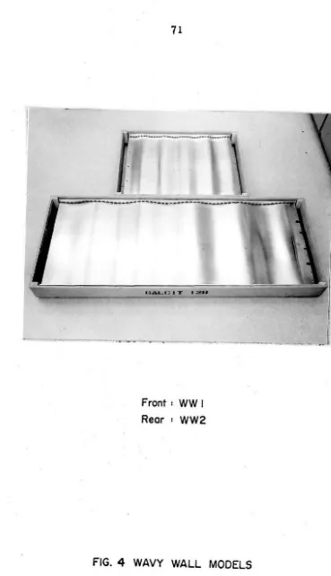
Wavy Wall Models

Two models were designed and built for the pres ent test, both with nominal amplitude to wave length ratio of O. 03. Each has five waves, with the following lengths:

WWl

A

= 12" WW2

(19)

drilled, with their centers along a sine curve of the desired amplitude and wave length. Two layers of aluminum sheeting were deformed to the sine -curve shape and held in place by pairs of rods spanning the frame through the holes on the sides. Epoxy cement was applied, in generous quantities, on the underside of the lower sheet, thus glueing the sheet, the lower rods and the frame into a solid unit. After the epoxy was cured, the upper rods and sheet were removed.

For the measurement of wall pres sure, a row of ports, O. 020 11 in diameter were drilled O. 5 11 off the centerline of the models. The spacing is 111 for WW1 and 0.75 11 for WW2. This operation was done on a milling machine to as sure accuracy in spacing the ports. At the time that the models were mounted on the milling machine, the wave form was measured with a 0.00111 accuracy indicator. It was found that because of the deformation of the rods, the actual amplitude of the wave is lower than planned. But, measurement in several trans-verse planes showed that the center 20 11 of the models were flat in this direction. The measured wave form is shown in Figure (4) from which it was found:

WW 1: a = O. 335 11 a/)...,. = 0.0279 WW 2: a

=

0.157 11 a/)...,. = 0.0261

Finally, the models were polished to a shiny, wax coated surface.

For a surface shape

= _{-a s}III \-)...,.-

. !21TX)

(20)

3

R

=

(1 +y/2)2

/I

Y

.9..

2

1

+

(2if

~

)

COS

2 (2ifX)2

-A

=

(2 ,2

if, . (2ifX)

-a

T)

SIn - -_A

The minimum (absolute value) of the radius of curvature is

R . = a

mIn

which for the two models give: WW 1: R . = I O. 3 II

mIn

WW 2 : R . = 5. 8" mIn

II. 3. Wind-Tunnel Boundary Corrections

The linearized velocity potential of inviscid flow over a wavy wallis (i.e. (8)):

-~

. (2ifX)

A

er

0 = V 0 a SIn

-1.-

e

On the other hand, for a channel formed by a wavy wall of the same amplitude and a straight wall at a distance H apart is:

-~

= Vo a sin

(2~x)e

A

y-H

4if

A

l+e

4ifH

l+e-

-1.-Though the wavy wall models are finite in length, the ratio of the two expressions given above will be used as a measure to the

(21)

Y.:.!i..

4rr Ie

l+e =

4rr H

-

_.-l+e It

For H

=

2411, and It

=

6 11 or 1211, this ratio is practically a unity near the wavy wall (y'" 0) and up to the center of the test section

(y'" iH). Hence it is concluded that the top wall effect is null.

II. 4. Pres sure Measurement

*

The heart of the pressure measurement system is a Statham transducer with a range of ± 0.2 PSID. The sensitive element of this transducer is a four arm strain gage bridge. The excitation voltage to the bridge is provided by a regulated D. C. power supply, operated with a battery connected as an external reference. See Figure (6).

This arrangement as sures excellent stability of the supply voltage. The output of the bridge is amplified and filtered, and then read by a digital voltmeter. The same voltmeter is used to adjust the bridge input voltage before each test.

A Betz, silicon-oil micromanometer, is used to calibrate the transducer. The readout is accurate to O. 02 mm. The electronic circuit that was described above was used during the calibration.

The transducer (P5TC-0. 2D-350) was calibrated at the beginning of the test giving the constant K

=

5.5017 gr/cm2/mV at 12V input.

The deviation from linearity and zero shift were less than 0.1% of full scale. Two calibration checks were done during the test, which showed deviations of less than O. 2~ in K.

(22)

II. 5. Calibration of the Test Section

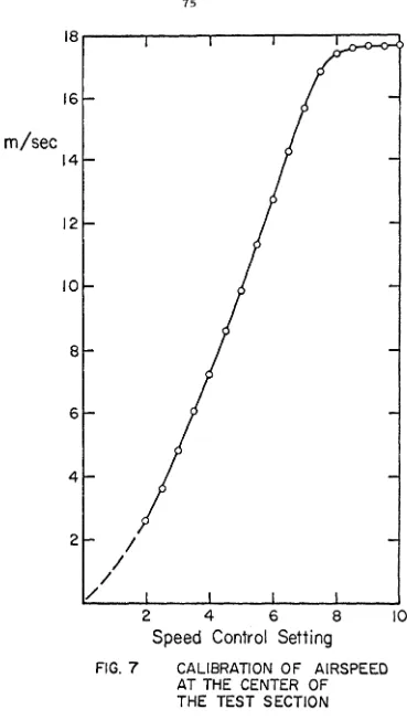
The O'oal ofthis calibration is to establish relation between the b

airspeed in the test section and the setting of the driving fanls speed control. Such relation is essential for the calibration of the hot-wire and pres sure probes, as will be dis cus sed below.

Calibration tests were run with plain floor TIlounted parallel to the ceiling, with a boundary layer trip T =

O.

5" TIlounted

6

11

up-streaTIl of the entrance to the test section.

A Pitot tube was TIlounted at S TN 5, at the center of the test section, aligned along its axis. The transducer and TIleasuring systeTIl des cribed in Section II. 4. were used to TIleasure directly the dynaTIlic pressure as the difference between the Pitot pressure and the static pres sure frOTIl the sidewall port at the saTIle station. The airspeed is

t d f 1 P

u

2

COTIlpU e rOTIl

P

d

=

"2 Figure (7) shows the result of the

calibra-tion.

Repeatability of the airspeed was tested by turning the tunnel on and off several tiTIles. Stability was tested by running it for a long tiTIle ( ... 1 hr.). Both tests showed that at speed control 7, variations in airspeed are within ± 1

%.

II. 6. COTIlpensation for Boundary Layer Growth

The thickening of the boundary layer along the walls of a parallel test section causes a reduction in the effective cross section area, by displaceTIlent effect. This forces the flow to accelerate and the static pressure to decrease in downstreaTIl direction. The effect is unwanted

(23)

In order to maintain a constant pressure test section, the floor is tilted such that it forms a slightly divergent tunnel. For complete cancellation of the unwanted pressure gradient, the increase in cross section area must be equal to the increase in boundary layer displace-ment.

The amount of divergence was determined experimentally for the four boundary layer trips that were used in the test. It was done according to the following procedure: The static pres sure was meas-ured along the center of the back side wall of the tunnel at STNls

6,

7, 8 and 9, with STN 5 as reference, while the exit end of the floor was lowered by h = O~ 111 and 211. Then, by interpolation followed by trial

c

and error the best h was found, for minimum variation of static pres-c

sure along the test section. Sample results (for T = 0.5") of the process, together with the geometrical data are given in Figure (8).

The values of h , for the other cases are: c

T (in) h c (in) O. 05 O. 7

0.25 0.5

0.50 0.9

O. 75 O. 7

(24)

All the results presented below were taken with floor tilted for best boundary layer compensation.

II. 7. Velocity Measurements

Airspeed measurements were made by means of hot wire ane-mometry. The equipment is a constant temperature, linearized output

>.'(

set made by DISA.

For the measurement of average velocity and turbulence level, type 55A25 miniature, straight prong, single sensor probe was used. The sensing wire is Pt-coated tungsten, 0.005 rrlm diameter by 1. 2 mm long.

Two channels of measurement were used. Each channel con-sisted of a constant temperature anemometer, a linearizer and an RMS unit, as shown in Figure (9).

The probes were calibrated at the center of the test section, under the same conditions as des cribed in Section II. 5. The results for three pro bes that were used in the test are shown in Figure (10).

A single element probe with its sensor parallel to the surface, does not distinguish between longitudinal (u) and normal (v) velocity components. Its output is proportional to the resultant velocity which is:

q =

--;z:

2

----;2«

V 2 h D d M S 1 Assume that u « U J v J t e . C. an R. . . va ues

of this signal are proportional to:

(25)

I

Q

= (U2 + V2)2

Q'

(

U

2

,2 V2

--;z

+ 2UV

-'-'l

= ₂ _{2 u} ₊

U2+V2 v

U2+V2 u v U +V

In order that distinction is made between results obtained by a single element and an X -array hot wire probe, notation (

Q,

Q') will be used for the first one.

The readout of the anemometer IS D. C. meter, the R. M. S. unit and the vertical position indicator were recorded on coding charts.

The data was manually key-punched for computer processing and plotting.

II. 8. Freestream Flow Conditions

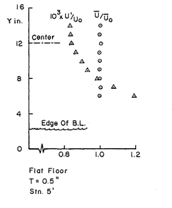
In order to find the uniformity of the flow outside of the bound-ary layer, and its turbulence level, velocity survey was perfo rmed using a single sensor hot wire probe. The survey was done above plain floor, at STN 5, with boundary layer trip T = 0.511

and covered the range from 611

to 14" of distance from the floor.

The results are shown in Figure (11), from which the following is concluded: The deviation of the average velocity, from its value at the centerline, does not exceed O. 5%. The free stream turbulence

level is 0 .. 83%, but it exists only above the centerline of the test section.

- /

(26)

III. TEST REFERENCE CONDITIONS

III. 1. Reference Boundary-Layer Profiles

As mentioned in the introduction, a trip was inserted about 611

upstream of the entrance to the test section in order to thicken the boundary layer. Square bars of different thicknes ses were us ed, ex-cept one case: T = 0.7511

• It was found that such a thick trip generated

velocity profile with practically no wake component and unusual turbu-lence distribution near the ed.ge of the boundary layer. After trial and error, a 0.2511

bar, mounted on 0.511 _{high legs gave good results.}

This combination trip is still referred to as O. 7511 _high.

The boundary layer on the plain floor was surveyed, by means of a single sensor probe, in order to provide knowledge about the on-coming flow and as reference to compare with. STN

6

and STN 7 were surveyed in order to serve as reference to WW2 and WW 1 respectively. This is illustrated graphically in Figure (12), At each station, survey was carried out for three trip heights according to the following table:

T U STN

61

STN 7

in. m/sec.

O.

05 15.54

+

0.25 15.43

+

0.50 15.43

+

0.75 15.41

+

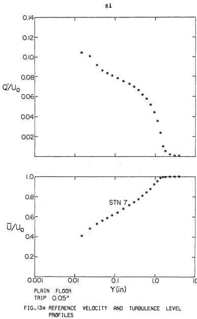
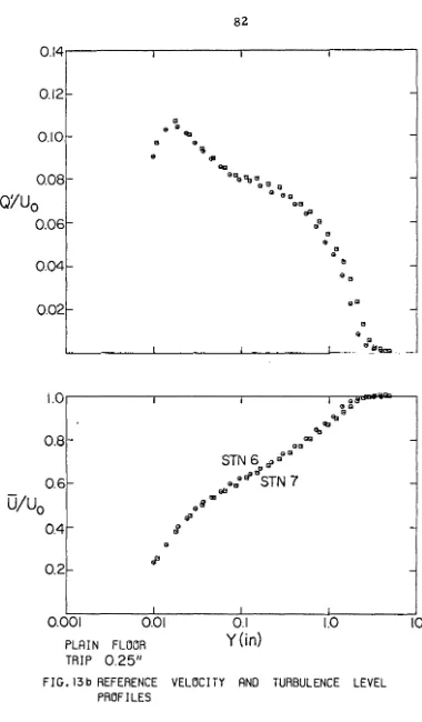
The results are shown in Figure (13), where normalized average velocity (U

Iv ) and turbulence level

(Q I

Iu ) are plotted against distance

e e

(27)

turbulence level of about Q I

lu

= o.

107 at a distance O. 01- O. 013"

e

from the wall, depending on boundary layer thickness.

III. 2. Law of the Wake Fitting to the Data

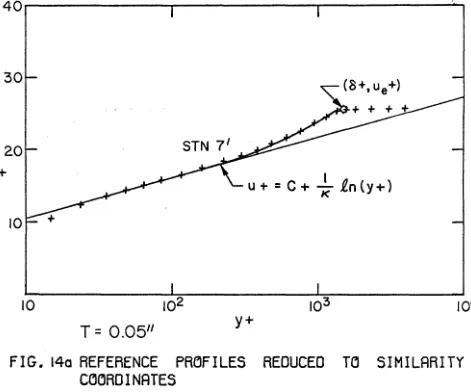
To gain qualitative knowledge about the reference boundary layer profiles they were analyzed by fitting Coles I (9) Law of the Wake

similarity profiles to the experimental data. Recall, from (9) _J the Law of the Wake:

u

C +

~

0n ( Y

:7 )

2 7T _sin2

(;

~)

_{(1 )}

=

+

u K

T

with: C

=

5. 0

K

=

0.41

Parameter 7T can be eliminated from (1) by using edge condi-tions:

u

=

u @ _y

=

5 e

2~ ue

~

_{0n (}

5:

T

)

(2 )

=

C

-K u

T

Substitute (2) into (1 ), and one finds:

Eq. (3) contains two parameters, namely u and 5. A computer

T

program was written to evaluate these parameters for least square deviation from the experimental data. Points with y+ = Y u

Iv

<

60

T

or ulu

>

1 were omitted from the fitting process. The program uses e

(28)

The best fit curves, together with the data, are shown in

Figure (14) for all reference profiles. The presentation is in universal coordinates, i. e. u+

=

u/u vs. y+ = Y u

/v.

The important parameters

'T 1"

are tabulated below:

T STN U'T 0 1T C

f

in. m/~ec in.

O. 05 7 0.61 1. 50 0.59 0.00301

0.25 6 0.59 1.

96

0.51 O. 00297

0.25 7 0.58 2.43 0.51

o.

00286

0.50 6 0.60 3. 08 0.21 O. 00306

0.50 7 0.59 3.41 0.23 O. 00298

O. 75 6 0.61 3. 70 0.23 O. 00293

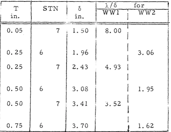
After knowing reference boundary layer thicknesses, it is pos-sible to summarize the range of ,,/0 parameter for the present test.

T STN 0

A/o

for

WW1 WW2

In. in,

..-O. 05 7 1. SO 8. 00

0.25 6 1. 96 3. 06

0.25 7 2.43 4.93

0.50 6 3. 08 1. 95

I

0.50 7 3.41 3.52

I

.

[image:28.535.138.422.525.743.2]

(29)

III. 3. Boundary Layer Thickness and Shape Factor ,~

The displacement thicknes s (6 ) and the momentum thicknes s (8), are uniquely determined by the thickness (6) and the wake compo-nent coefficient

(iT).

But, since numerical integration was incorporated in the data processing program, the two quantities were evaluated this way. By definition:

=

u , l u )

U

~ 1 -

u

dy

e e

e

=

The results, together with the shape factor H = {)

*

/e

are sum-marized in the table below.

Note that the reference profiles are not similar. The shape factor varies from 1.25 to 1. 34.

T STN 6 f/~

e

H

in. in. in. in.

0. 05 7 1. 50 I

I

0.226 I I

o.

189 1. 34

1

0.25 6 1. 96

i

!

0.282 0.213 1. 33

I

0.25 7 2.431 O. 344 0.262

r

.

1. 31

I

0.50 6 3.08 0.356 0.284 I 1. 25 0.50 7 3.41 0.388 0.307 1. 27

I ;

0.3341

I

0.75 6 3.70)0.425 1. 27

I

(30)

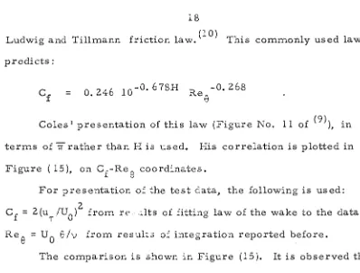
Ludwig and Tillmann friction law. (10) This commonly used law predicts:

= 0.24610-0.678H

R

ee

-0.268

Coles I presentation of this law (Figure No. 11 of (9)), in

terms of

Tr

rather than H is used. His correlation is plotted in Figure (15), on Cf-Re

e

coordinates.

For presentation of the test data, the following is used: 2

C

f

=

2 (uT ,IVO) from re,llts of fitting law of the wake to the data;

Re

e

= V 0

e

Iv

from results of integration reported before. [image:30.523.67.465.81.383.2]

(31)

IV. MEASUREMENTS AND RESULTS

The models were mounted in the test section with their front end at S TN 5, as shown in Figure (12). The leading edge of the models is at the same height as the flat plate that composes the upstream part of the floor. In the cas e of the short WW2, another plate was installed behind the trailing edge to complete the floor to the full length of the test section.

The test was conducted with floor dive rgence as for the plain floor (Section II. 6).

IV. 1. Wall Pres sure

The distribution of static pressure on the two models was measured by a series of ports, 0.02011 _{in diameter, located 0.5}11 _off

of the center line. The ports are spaced 111 apart for WW1 and 0.75"

for WW2. The measurements were done for the different boundary layer trip heights, as mentioned in Section Ill. 2.

The transducer and measuring .scheme that were described in Section II. 5 were used. The reference pressure is the port located at STN 5 on the side wall of the test section. The wall ports were con-nected in turns to the transducer.

The results were reduced to the non-dimensional form:

Cp w =

(32)

Since the effect of boundary layer thickness upon wall pressure was found to be ve ry small, the complete distribution is shown for one case only (T

=

0.511

) in Figure (16). For the two models, we

observe that the first and last waves show lower pressure peaks than the three center waves that are about equal in shape and amplitudes.

This reflects the surface shape as mentioned in Section II. 2. Note that the first wave of WW2 had a local kink at x'"'" 5". This gave ab-normal result that was not included.

A summary of all the cases for wave No. 3 only is given in Figure (17), together with results from other sources. The following observations are made:

(i) The maximum positive pressure peak is lower by 31% for WWl and 20% for WW2 from the maximum negative value.

(ii) The positive part of the pressure curve occupies more than half wave: it covers 1880 for WW1 and 1910 for WW2.

(iii) The invis cid, uniform flow, linearized theory for flow over a wavy wall predicts

=

4'iT a

r

For the present models this gives

WW1:

I

e

I

Pw'v=O

=

0.352

WW2: = 0.340

(33)

! Cp I

I

Model

I

STN C pw(meas.)

I

CPw(v=O) w(meas. )

I

WW 1

i

max. 0.175

!

0.497

i

WW 1

I

min. -0.255

!

O. 725

I

WW 2 max. 0.155

I

0.440

I

WW 2 I min. - O. 195 0.554

I

The asymmetry in pressure distribution gives rise to form drag, defined by:

A

CD

=

1

f

Cp Y I dx

P

X"

w s

o

This integral was evaluated graphically for T = 0.5". The results for the two models are:

WW 1: CD = O. 001 2 P

WW2: CD = 0.0017 P

Comparison between the present results and those of Kendall( 7 )

and Motzfeld ( 6 ) shows consistency in the trough area. On the other hand, present measurements show lower crest pressure than expected from Kendall IS presentation of ~.educed pressure coefficient (Figure 4

of ( 7 ).

(34)

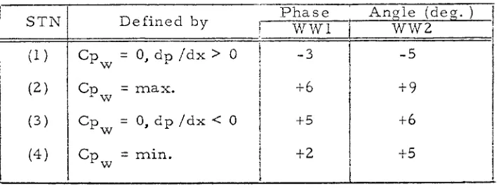
STNi Defined by Phase Angle (deg. )

I

WWl WW2

(1 ) Cp

=

0, dp Idx

>

°

-3 -5

w

(2 )

I

Cp

=

max. +6 +9

w

(3 ) Cp

=

0, dp Idx <

°

+5 +6

w

(4 ) Cp

=

min. +2 +5

w

IV. 2. Velocity Profiles

The first field survey was the measurement of average velocity profiles and turbulence level, using a single sensor hot-wire probe. Each of the two models was surveyed at the four stations, listed in the table given above.

The results of the survey are presented in two forms. The first (Figure (18)), on a linear y-scale with velocity and turbulence profiles, are shown at the station where they were taken. For comparison, the plain floor profiles and for reference the wall pressure are also shown. In the second form (Figure (19)), log (y)-scale is used, as is common for presentation of turbulent boundary layer data.

The following observations are typical to all the cases tested. (i) At the crest, the velocity profiles are full at a very close distance from the wall. A typical value is Q

I

u

°

=

0. 7 at y

=

O. 025".

(ii) On the other hand, the trough profiles grow slowly near the wall. This shows also in a relatively low (Q I

lu

0 "-' O. 08) turbulence

level nea r the wall. At a distance of 0. 15 II froITl the wall turbulence

[image:34.522.108.465.125.260.2]

(35)

(iii) The two profiles corresponding to CPw

=

0 have the same shape for distances from the wall larger than O. IS". Only in the wall layer they corne apart, which shows also in differences in turbulence level near the wall.

(iv) Among the four stations surveyed, the largest turbulence level for WW1 was found at the crest, with

O'/U

O

=

0.12. For WW2, it takes place at the uphill slope with Q '/_UO

=

0.13.

(v) At distances from the wall where the reference profiles possess a semilogarithmic section, the present pro-files show a small degree of waviness. This phenomena will be observed throughout the data that will be discussed below.

(vi) There exists a correspondence between the slope

au / ay of the mean velocity profiles and the turbulence intensity. High slopes are always accompanied by increased turbulence intensity (i. e. the crest profile near the wall) while low slopes are correlated to reduced intensity (i. e. the trough profile near the wall).

Effect of Boundary Layer Trip

(36)

It is obs erved that for the two models and the four stations of survey, the behavior of the wall layer is almost independent of the boundary layer thicknes s. This shows up for the mean velocity and the turbulence intensity distributions at distances from the wall up to 0.211

DeveloDment of the Flow !

The two models in the present test are composed of five waves each. Only the center wave was surveyed for velocity and turbulence level distribution. A question rose on how the reported results represent a situation over a long train of waves. In other words, how many waves does it take for the boundary layer to become periodic.

To answer this question, waves No. 2 and 4 of WW1, with T = 0.50", were surveyed at four stations, as defined for wave No.3. The results for velocity distribution are

(37)

Test for Two -Dimensionality

Final test for the quality of the results is for two -dimensionality of the flow. This test was conducted for WWl with T

=

0.50" at the

four stations of survey. A dog-leg extension was attached to the arm of the traverse mechanism. The probe was attached to the extension, thus enabling the survey at 4" from the centerline of the test section.

Results are presented in Figure (22), together with the center-line profiles, for comparison. Again, small differences are found, but there is no change in shape that implies deviation from two-dimensionality at the center core of the test section.

IV.3. Wall Stres s

Preston Tube Probe

A flat-mouth preston tube was used to evaluate the wall shear. When the tip of such probe touches a wall, it measures an overpressure

. (11) (12)

gIven by: '

p - p

=

p w

K

d2

J

s

t

2

p u do

where S is the area of the opening of the probe and d is its cha racter-istic height and the calibration factor K is a function of the shape of the probe and the velocity profile. In the case of similarity profiles, for which u/u

(38)

no siITlple calibration can be provided for the desired K. To overCOITle this probleITl, it was decided to use a probe which will be fully sub-ITlerged in the linear portion of the viscous sublayer. Therein, the velocity is given by:

u

,.

=

\! y

and the calibration factor K can be considered as a constant.

The thickness of the viscous sublayer can be estiITlated froITl the results of a siITlilarity-law fit to the plain floor boundary layer profiles (Section III. 2). For exaITlple, for T = 0.25", u,. = 0.6 ITl/sec.

Hence:

y

=

O. 001 y+

If the viscous sublayer extends up to y+ = 5, say, its edge is 0.00511

above the surface.

But, froITl the results of the previous section, wall shear is expected to reach a ITlaxiITluITl at or near the crest. This ITlaxiITluITl is accoITlpanied by the thinning of the sublayer. To estiITlate the ITlin-iITluITl thickness of the sublayer, wall shear distribution ITleasured by Kendall (Figure 15 of Ref. (7)) is used. There it was found that the ITlaxiITluITl value of C/C

f is 1. 3. But, for y+

=

5: o

Yl u

,.

=

-Y uTI

1

=

(C/C

f )2

1

(39)

Hence the smallest sublayer thickness is expected to be:

Ymin = 0.0044

11

Finally, an evaluation is made of the effect of streamwise pres-sure gradient on the deviation from a linear laminar sublayer profile. In the sublayer (cf. (11), (12»:

u =

'T"

w

+

1 ~ 2

p v y 2pv dx Y

+ ..•

which can be rewritten in a non-dimensional form as:

u

u'T"

=

+ [

1

Y 1

+

AU

4 _ _ 'T"

V

d CPw

+

]

y

+ ...

d ( ~ )_t~;:

'

The most severe case is WW2, with

A

=

611

• There, based on a

flat floor friction velocity:

- -

=

6000

v

the normalized wall pres sure gradient parameter, from Figure (17) is:

dCp w

= 1.2

+

At the edge of the viscous sub1ayer (y = 5) we find

1

AU 4 _'T"_

V

= ₄₀₀₀1

Hence, the nonlinear term can be neglected compared to the leading,

+

(40)

The probe was designed to have the upper edge of its opening less than 0.0044" from the wall. Its general dimensions and a com-parator picture of its front end are given in Figure (23).

Method of Measurement

Becaus e of the large variation in wall static pres sure, the measurements were obtained by recording the pressure difference

(p -p ) at each station that has a static pressure port. At each

p

w

station, the tip of the probe was aligned on a normal to the flow direc-tion at a distance O. 7" to the side of the static port. The measuring

schematic of Figure (6) was used, with the Preston tube connected to one side of the transducer and the wall port to the other. This arrange-ment is shown in Figure (23c).

The calibration of the probe was made on the plain floor, under the same conditions used for the measurement of the reference velocity profiles. The value measured is given by:

=

-Z

K

II

z

p u 2 da d S

=

2

.!S....e...

(au)

J

y2 da 2 d 2

ay

w, 0 S

K I

P

<::l 2 2 (~) d

2

ay

w, 0

=

This can be rewritten in a non-dimensional form 2

(p -p ) d

P w 0

2 P

v

=

(41)

2

P -p ) d

P

w 0

2 pV

=

Therefore, the ratio of skin friction coefficients becoznes

=

T

w

T

w o

The sensitivity of the pressure difference (p -p ) to the

inclina-p

w

tion angle of the probe was exaznined in the range 0 ~ ~ ~ 8°. The re-suIts given in Figure (23), show alznost no change in this range.

The znagnitude of change in p caused by the proxiznity of the w

probe was also zneasured on the plain floor. The probe was znoved acros s the boundary layer until it touched the floor and changes in p were recorded. The corresponding changes in Cp are also shown

w w

in Figure (23). Since 6 Cp /Cp is less than 2%, no correction for

w p

this effect was incorporated in the data reduction.

A few factors znake this zneasureznent difficult and sus ceptible to errors. 1) At the slopes, where dp /dx is large, sznall deviations

w

of the tip of the probe, frozn the transverse line, can cause appreciable error. 2) At the valley, optical inspection of the orientation of the probe at the surface was iznpossible. 3) Turning the flow on and off znany tiznes during the test can cause changes in U .

o

Measureznents

(42)

fixed between the existing ones. The results, in a non-dimensional form C/C

f are presented in Figure (24).

o

The scatter in the data is large, reflecting the difficulties mentioned above. Therefore, no consistent trend of the effect of boundary layer height can be discerned from the present results. Nevertheless, the shape and phase angles of the wall stress distribu-tion are apparent.

WWl: The wall stress reaches a peak with C/C

f

=

1. 18 and o

a phase shift of 45° upwind of the crest. The minimum value is C/C

f = 0.63, with a phase shift of 30° upwind of the trough. o

WW2: The maximum wall stress is C/C

f = 1. 25, a phase shift o

of 20° upwind of the crest. Proceeding downwind, the curve declines sharply to a value of 0.7, at about 50° downwind of the crest. At the center of the downhill slope, a second, low peak is observed, followed by a gradual increase, from a value of O. 65, along the uphill slope to the next peak.

*

Kendall found a b('havior similar to that of WW2 in an un-published extension of his moving wave experiment.(7) This occurred with waves moving into the wind, hence increasing wall pressure

gradients.

The wall shear curves have been integrated to find the skin friction drag coefficient defined by:

=

.!.

J

A C dx

C_Df A 0 p (cos y''''''I)

The results are: WWl: CD = 0.0027

f

WW2: CD = O. 0028 f

(43)

The results so far, including wall pressure, shear stress and velocity profiles, do not show a significant effect of the ratio 6/)",. It was therefore decided to proceed and do the flow field surveys with one

boundary layer trip only. T = 0.511 _{was chosen arbitrarily for the rest}

of the test.

IV. 4. Static Pressure Survey

The distribution of static pressure along the surface of the wavy walls was described in Section IV. 1. Here the technique and results

of the static pressure survey within the boundary layer are reported. The knowledge of the distribution acros s the boundary layer is of

importance, since its gradients considerably alter the velocity profiles. The measurement of static pressure in non-uniform flow fields is known to be difficult. In the present investigation this difficulty is amplified because of the curvature of the streamlines and the

conse-quent changes in the turbulent quantities. It was decided, therefore, to try three possible probes and find which of them demonstrates mini-mum sensitivity to flow direction and turbulence.

The calibrations of the three probes, whose forms are described below, was carried out in two steps:

(i) Calibration in the free stream to find sensitivity to

airspeed or to Reynolds number. This was accomplished with plain floor, using boundary layer trip T

=

0.50", and with the probe oriented along the cente rline at STN 6. (ii) Calibration in the boundary layer in order to determine

(44)

using the plain floor, tilted to provide constant pressure for boundary layer trip T = O. 50". Recall that Figure

(13c) describes the average velocity and turbulence level for these test conditions.

Disc Probe

This probe is recoITlITlended by Bryer et. al. (15) for survey of two-diITlensional flow fields where the direction of flow is not well known. Results of calibration of such probe (Figure 12 of (15)) show that it ITleasures Cp = -0.12 and that this value reITlains alITlost

con-ITl

stant for angles of attack in the range ± 20° .

The probe that was tried in the present test is described in the upper part of Figure (25). It was aligned carefully along the centerline of the test section, with its plane perpendicular to the floor.

Results of the calibration in free streaITl are shown in the lower part of Figure (25). The average ITleasured pressure coefficient is Cp = -0. 14, and the deviations do not exceed ± O. 003 in Cp .

ITl ITl

The results of pres su re coefficient, ITleasured within the bound-ary layer are presented in two forITls: The first is norITlalized by edge velocity U and the second by local velocity U

o

(1) CPITl

,

0 =

P-Po

~U2

2"

P

0

(2) C

=

P -Po

PITl ~ 1 -2

I 2" P U

(45)

have a strong gradient near the wall, which reflect interference. The Cp curve grows monotonically toward the free stream value outside

m, 0

the boundary layer, while Cp ~ has a peak at h = 0.5" which is appar-m, AI

ently caused by the turbulence.

Sphere Probe

This probe consists of 1/8" diameter sphere with four equally distributed pres sure taps inclined at 42° with respect to the free stream direction. The inclination angle of 42° was chosen because the surface p res sure vanishes at that location for subcritical Reynolds numbers .(16)

Indeed, calibration in free stream (Figure (27» shows almost zero pres sure coefficient. Actual values range from Cp

=

-0.001 at

m U = 7.5 m/sec to Cp = 0.003 at U = 15.7 m/sec.

o m 0

Calibration inside a boundary layer (Figure (28» shows a strong gradient near the wall, a plateau of Cp = O. 032 that ranges from

m

h =

o.

9" to h = 2. 0", and a gradual decrease toward the free stream value for h

>

5. 0".

Needle Probe

This is a sting type static pressure probe constructed from 0.042" O. D. tubing. It has a rounded nose and three pressure taps located at a distance t

=

10d from the front end. It is described in Figure (29).

Results of the free stream calibration show that the measured pressure coefficient is 0.0075 independent of velocity.

(46)

variations across the layer, but the changes about the average value of Cp = O. 0055 do not exceed 6 Cp = ± O. 002. This range of

m m

variation is tolerable in use.

From what was des cribed above. it is clear that the needle static probe gave the best performance by being less sensitive than the other two probes to turbulence and proximity of the wall.

The final test for this probe was to find its sensitivity to incli-nation of the flow. This was done for angles of attack of +5° and -5°. The results of this test are shown in Figure (30). We observe from the plots the same unpredicted variation across the boundary layer as in the zero angle of attack case. The average values of pressure co-efficient are:

e

CPm

-5 .003

0 . 0055

+5 .008

The s ca tter I in all cases, is ± O. 0002 about the average. But the differences between the averages and the scatter are small enough to permit the use of this probe in the present test.

Results

(47)

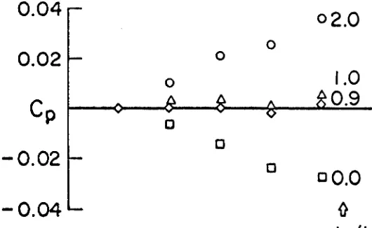
The results, normalized to a form of static pressure coeffi-cient, are shown in Figure (31) for the two models. The following observations are made:

(i) For the two models and the two stations where Cp = 0,

w

the static pressure remains nearly zero over the entire layer, reach-ing a value of -0.01 or less in the free stream.

(ii) WWl: At the trough station a layer of constant static pressure O. IS" in height is observed. Proceeding the static pressure declines until above h

=

0.55" it decays exponentially. At the crest, the layer of constant static pressure is O. OS" thick, followed almost immediat ely by exponential decay.

(iii) WW2: No tendency to form a layer of constant static pressure near the wall is observed for this model. Static pressure

curves decay exponentially above O. 35 II distance from the wall at the

trough and 0.25" distance from the wall at the crest.

Because of the observed exponential form of the pressure curves away from the wall, a curve fit was obtained whose form was chosen from the uniform, inviscid solution for flow over a wavy surface.

Corrections made for the actual reduced amplitude of the wall pressure and for the existence of a layer of constant pres sure near the wall, yielding the function

-a(y-A)

Cp (y)

=

Cp e

s w

(48)

Model WW1

WW1

WW2 WW2

STN

(2 )

(4 )

(2 )

(4 )

A in. 0.45 O. 12

0.20

O. 10

Note that the values of A are very close to the displacement thickness of the boundary layer at the same locations.

IV. 5. Total Pres sure Survey

In principle, knowing both the velocity and the static pres sure distributions acros s the flow field, one can determine the total pres-sure using Bernouli's equation. Even so, it was decided to meapres-sure the total pressure because direct measurement is more accurate and

can provide a check for the quality of the static pressure.

In order to get good resolution, a flat mouth Pitot tube was used with opening 0.010" high. Measurements were made with p as

o reference. The two models with T = O. 5 ", were surveyed, each at the standard four stations.

The analysis of the results of the total pressure survey are given in the next chapter. Here they are used to check the static pressure distributions discussed above.

Check of the Static Pressure Distribution

(49)

= Cp

+

(D/U

)2

s 0

Therefore, a cOITlparison is ITlade between the direct

ITleasure--

2

ITlent of CPt and the value calculated froITl the SUITl Cps

+

(U /U 0) .

(Sections IV. 4. and IV. 2.). Two typical plots are given in Figure (32). It is observed that the differences do not exceed O. 025 out of 1. O. All other cases show the saITle accuracy or better, and therefore are not shown.

IV.6. X -Array Probe Survey Probes

The ITlain purpose of using an X-array hot-wire probe is to ITleasure Reynolds stres ses and related quantities, i. e. ITlixing length and eddy viscosity.

DISA type 55A38 probes were used. The two sensors are 1. 2 ITlITllong, 0.005ITlITl diaITlecer, Pt-plattedtungstenwires, placed In an X-array. Two probes were used during the investigation. One, a standard 55A38, was used to survey the flat plate and WWl. For WW2 a special probe with bent prongs was built in order to allow ITleasureITlent very close to the wall without exceeding the range of linearity. This special probe has the saITle sensors as the standard one and is shown in Figure (33).

(50)

signals. Two RMS units are used, in turns, to record four signals:

]';1' E"'2'E"'s = (E

1 +E 2 ), Ed

=(E~Ez)'

Details about the utilization and calibration of the probes are presented in Appendix A.

If the calibration constants of the probes are defined by

El = Au

+

Bv

E2 = Cu - Dv

where E

I, E2 are the linearized outputs in volts and u, v are the axial and normal velocity components in m/sec., then their results of the calibration gives;

Probe: X-I

Calibration constants: A = 0.402

C = 0.399 Range of linearity: ± 230

Probe: X-S

Calibration constants: A = 0.462

D = 0.457 Range of linearity:

+

230

, _200

Stations of Survey

B = 0.556

D = 0.423

B = 0.475

D = 0.490

Data presented above showed a strong modulation of the flow quantities over the wavy wall models. Therefore, it was decided to increase the number of stations of survey for the present measurement.

The boundary layer was surveyed at eight stations, four of which are

(51)

the distributions of the turbulent quantities is obtained.

Comparison with the Results of a Single Element Probe

Because of the tedious process of calibration of the X-array probes, the results are compared with those obtained by a single

element probe (Section IV. 2. ) in order to gain confidence in the

accuracy of the present measurements. Five sample cases are shown in Figure (35). The first one is the flat plate case, and the other four

are the standard stations of survey for WWl. The two velocity com-ponents, and the turbulent quantities U', V' and u I v I are shown on a

log (y) scale as inSection IV.2. The following observations are made: (i) Longitudinal velocity component, U, and turbulence

intensity, U~ differ by no more than 5,% of their maximum values from their counterparts Q and Q I measured with a single element probe. In spite of these small differences, the two curves always show the same trends.

(ii) Normal velocity component, V, is practically zero in the case of the plain floor, and at the crest and trough stations of the wavy wall, as expected. At the downhill and uphill stations, V has negative and positive values respectively, that diminish tm,\,lrn the edge of the boundary layer. The ratio V

tIT

near the wall agrees with the local

surface inclination.

(iii) For the case of the plain floor the Reynolds stress is

constant near the wall with a value

-'-'/1

u

2

(52)

This value is in good agreement with the wall shear coefficient C

f = 0.00306 found in Section III. 2. by fitting Cole's Law of the Wake

to the velocity profiles.

Turbulent Intensities

The results of the measurements of the two turbulent intensities,

v'

and V', are presented in Figure (37). The distributions of the turbulence intensities and the shear stress that will be discussed in the following section, exhibit oscillations of damped amplitude super-imposed on the reference flat plate boundary layer distributions. This wave phenomena will be related in Section V. 5. to the Rayleigh prob-lem. Here, the important findings are summarized.

(i) At distances exceeding 1. 2" for WWI and 0.6" for WW2, above the line connecting the centers of the waves, the two turbulence intensities are practically independent of the station along the surface wave and are given by the reference case. The changes in these quan-tities are large near the wall and decay as the outer layer is approached. Qualitatively, the changes are the same for the two models, but it is apparent that the normal gradients in WW2 are larger than those in WWl.

(ii) In the vicinity of the trough, the normal distributions of V'

increase with increasing y, reaching a peak for which V'

lu

= 0.05 at o

(53)

where a value Vi

lu

= 0.05 is measured at the points closest to the o

wall. This local maximum again approaches the reference distribution in an 0 sci lla to ry manne r.

(iii) In the vicinity of the wall, the oscillatory behavior of U ' is

I

more pronounced than that of V. The distributions reach a peak near the wall at the station just downstream of the crest. The maximum measured values are U'IU

=

0.130 for WW2. Proceeding outward

o

at the same station, the distributions decrease below the reference value, form a second peak and then merge into the reference distribu-tion. Further downstream, on the downhill slope, the peak closest to the wall flattens somewhat and the intensity is reduced. At the trough, a flat maximum with U'

Iu

=

O. 11 is found at a distance y

=

O. 25" for

o WWl and y = 0.1611 _{for WW2.}

Turbulent Shear Stres s

The turbulent shear stress distributions given in Figure (38) show large variations across the layer as well as along the wall wave. The oscillatory nature of the normal distributions is apparent at all stations; the amplitude of oscillation about the reference curve being much larger than noted for the turbulent intensities in each cas e.

(i) As in the case of the turbulent intensities, the shear stress distribution is practically independent of longitudinal position at dis-tances exceeding 1. 2" for WW 1 and O. 6 II for WW2, above the mean

(54)

(ii) The downhill slope of the wave is characterized by a layer of high shear stres s near the wall, followed by a damped os cillatory behavior with increasing y. Just downstream of the crest, the maxi-mum measured C

T

=

O. 0072 is found adjacent to the wall. Further

downstream the layer thickens until at the trough it is O. 5" wide with a peak value C

=

O. 005. At the next station a rapid change takes

T

place, i. e. the layer exhibits a reversed curvature forming an S shape distribution adjacent to the wall. This profile evolves on the uphill slope into a dip; i. e. C

T """ 0 close to the wall, followed by a shallow

peak. At the crest, the dip begins to flatten, and it is followed by a rapid change from a dip to an overstress layer at STN (4i).

Mixing Length and Eddy Vis cosity

The mixing length is defined by the equation

_ u'v' = 1,2

(~

Hence, for the evaluation of1"

aU /

oy must be computed from the data. In order to overcome the difficulty associated with differentiating ex-perimental data, smoothing was introduced graphically for y

>

I". In addition, in the vicinity of the crest the velocity profiles exhibit a flat maximum near the edge of the layer. Because the derivative vanishes there, causing unacceptable errors, this part of the data was ignored in the evaluation of the mixing length.

(55)

I I

U V

Since the results of Appendix B are not conclusive, the value k = 10 was chosen arbitrarily for computations. As will be explained in detail below, the correction for curvature is not l