The spatial ecology of coral reef fishes

Full text

(1)ResearchOnline@JCU. This file is part of the following reference:. Welsh, Justin Quentin (2014) The spatial ecology of coral reef fishes. PhD thesis, James Cook University.. Access to this file is available from:. http://researchonline.jcu.edu.au/40758/ The author has certified to JCU that they have made a reasonable effort to gain permission and acknowledge the owner of any third party copyright material included in this document. If you believe that this is not the case, please contact ResearchOnline@jcu.edu.au and quote http://researchonline.jcu.edu.au/40758/.

(2) The Spatial Ecology of Coral Reef Fishes. Thesis submitted by Justin Quentin Welsh Bsc (Hons) James Cook University August 2014. for the degree of Doctor of Philosophy in Marine Biology School of Marine and Tropical Biology and ARC Centre of Excellence for Coral Reef Studies, James Cook University, Townsville, Queensland, Australia.

(3)

(4) Statement of Access. I, the undersigned, author of this thesis, understand that James Cook University will make this thesis available for the use within the University Library and, via the Australian Digital Thesis Network, for use elsewhere. I understand that as unpublished work a thesis has significant protection under Copyright Act and; I do not wish to put any further restriction on access to this thesis.. __________________________________ Signature. ___________________ Date. i.

(5) Declaration of Ethics. This research presented and reported in this thesis was conducted in compliance with the National Health and Medical Research Council (NHMRC) Australian Code of Practice for the Care and Use of Animals for Scientific Purposes, 7th Edition, 2004 and the Qld Animal Care and Protection Act, 2001. The proposed research study received animal ethics approval from the JCU Animal Ethics Committee Approval Number #A1700.. __________________________________ Signature. ii. ___________________ Date.

(6) Statement of Sources. I declare that this thesis is my own work and has not been submitted in any form for another degree or diploma at my university or other institution of tertiary education. Information derived from the published or unpublished work of others has been acknowledged in the text and a list of references is given.. __________________________________ Signature. ___________________ Date. iii.

(7) Electronic Copy Declaration. I, the undersigned and author of this work, declare that the electronic copy of this thesis provided to James Cook University Library is an accurate copy of the print thesis submitted, within the limits of technology available.. __________________________________ Signature. iv. ___________________ Date.

(8) Statement on the Contribution of Others. This thesis includes some collaborative work with my supervisor Professor David Bellwood (James Cook University) as well as Dr Rebecca J Fox (James Cook University), Dr Christopher HR Goatley and Dale Webber (Vemco, Canada). While undertaking these collaborations, I was responsible for the project concept and design, the majority of data collection, analyses and interpretation, as well as the final synthesis of results into a form suitable for publication. My collaborators provided intellectual guidance, equipment, financial support, technical instruction, statistical advice and editorial assistance. Data for chapter 4 was derived from previously unpublished data collected by Prof. David Bellwood, however, I was responsible for the data analysis, interpretation and final synthesis of the results into a form suitable for publication. Financial support for the project was provided by the Australian Museum and Lizard Island Reef Research Foundation, the James Cook University Graduate Research Scheme and the Australian Research Council Centre of Excellence for Coral Reef Studies. Stipend support was provided by a James Cook University International Research Scholarship. Financial support for conference travel was provided by the Australian Research Council Centre of Excellence for Coral Reef Studies.. v.

(9) Acknowledgements. I would like to start by acknowledge my supervisor, Professor David Bellwood. Throughout my career as a researcher you have been an unwavering source of encouragement, guidance and support. Words cannot express my gratitude to you for everything you have done for me. Furthermore, I would like to extend a special thanks to all my collaborators; Christopher Goatley, Kirsty Nash, Dale Webber, Rebecca Fox and Roberta Bonaldo. All of you have been an inspiration to me throughout my candidature and I will forever appreciative for your support, advice and patience. As with any project involving fieldwork, this would not have been possible without the tireless efforts of many field assistants. Thank you to Roberta Bonaldo, Yolly Bosiger, Simon Brandl, David Duchene, Christopher Goatley, Sophie Gordon, Jess Hopf, Simon Hunt, Michael Kramer, Susannah Leahy, Carine Lefèvre, Oona Lonnstedt, Mat Mitchell, Chiara Pisapia, Chris Pickens, Justin Rizarri, Derek Sun, Tara Stephens, John Welsh and Johanna Werminghausen for your time, energy, encouragement and friendship during countless hours of data collection. I am also very grateful to the staff at the Lizard Island Research Station, and Orpheus Island Research Station; Lyle Vale, Anne Hoggett, Lance and Marianne Pearce, Bob and Tanya Lamb, Stuart and Kym Pulbrook, Kylie and Rob Eddie, Lachin and Louise Wilkins and Haley Burgess. Your assistance and support made this project possible. My thanks are also extended to a number of other people who were invaluable along the way. I would like to thank; Sean Connolly, Jess Hopf, Marcus Sheaves, Richard Rowe, Steven Swearer and Vinay Udyawer for analytical and statistical advice; Roberta Bonaldo, Simon Brandl, Howard Choat, Christopher Goatley, Jen Hodge, Jess Hopf, Charlotte Johansson, Zoe Loffler, Roland Muñoz, Jenn Tanner and one anonymous reviwer for helpful discussion and comments on the text; Michelle Heupel and Colin Simpfendorfer for their valuable insights and for providing data from AANIMS receivers. Furthermore, I would like to extend a special thanks to all those who worked behind the scenes to make research possible; G. Bailey and V. Pullella for IT support, R. Abom, G. Bailey, G. Ewels, P. Osmond and J. Webb for boating, diving and logistical support; J. Fedorniak and K. Wood for travel assistance; D. Ford and S. Frances for a number of matters; and S. Manolis for purchasing.. vi.

(10) This research was made possible due to the generous support of many funding bodies. A special thanks goes out to the Australia Museum and Lizard Island, who supported this research through a Lizard Island Research Station Doctoral Fellowship. Valuable funding was also provided by the James Cook University Internal Research Awards and Graduate Research Scheme, as well as the Australian Research Council through Prof. David Bellwood. Furthermore, many thanks are extended to James Cook University who provided a Postgraduate Research Scholarship for the duration of my candidature. I am also very grateful to my close friends Karina, Jen, Ingrid, Jess, Charlotte, Jo, Zoe and Derek. You were not only a source of happiness and kindness during my candidature but also endless inspiration and encouragement. I am also extremely thankful to the members of the Reef Fish Lab. A. Hoey, B. Fox, C. Lefèvre, C. Johansson, C. Goatley, C. Heckathorn, M. Young, M. Kramer, J. Johansen, J. Hodge, J. Tanner, K. Chong-Seng, K. Nash, P. Cowman, S. Brandl and Z. Loffler for all your shared expertise and enthusiasm. A very special thank you goes out to my two families in Australia, The Bellwoods (Dave, Orpha, Hannah and Oli) and Hunts (Alan, Kerry, Kym, Annie, Emily and Simon). You truly have made me feel at home on the other side of the world. To my family back in Canada, dad, mom and Jazzy, I cannot thank you enough for your words of wisdom and kindness and most of all, for always being there for me. It is because of you that I was able to realize my dream. Last but definitely not least I would like to thank my partner, Simon Hunt. The support, friendship, patience and especially love you have shown me have been my greatest source of motivation. With you beside me, anything is possible.. vii.

(11) Abstract. Movement is a fundamental component of a species’ ecology and the study of space use in organisms has a long-standing history as a conservation tool. Within an ecosystem, numerous functional processes are conferred by taxa, and are essential to maintain stable ecosystem processes. The application of functional roles is, however, bound by the home ranges of the taxa responsible, and thus, the spatial ecology of organisms is of great significance to ecosystem health. Coral reefs are among the most vulnerable ecosystems to degradation and yet, the spatial ecology of key species which support coral reef resilience remain largely unknown. In this thesis I therefore endeavoured to quantify the spatial ecology of functionally important coral reef herbivores to further our understanding of ecological processes. Passive acoustic receivers are commonly used to remotely monitor animal movements in the marine environment. The detection range and diel performance of acoustic receivers was assessed using two parallel lines of 5 VR2W receivers spanning 125 m, deployed on the reef base and reef crest. The working detection range (distance within which > 50% of detections are recorded) for receivers was found to be approximately 90 m on the reef base and 60 m on the reef crest. No diel patterns in receiver performance or detection capacities were detected. These results are in contrast to those in non-reef environments, with coral reefs presenting a unique and challenging environment for the use of acoustic telemetry. Using a dense array of passive acoustic receivers, the maximum potential areas occupied by the schooling herbivorous fish, Scarus rivulatus, was quantified over 7 months. Despite schooling, all S. rivulatus were site attached. On average, the maximum potential home range of individuals was 24,440 m2 and ranges overlapped extensively in individuals captured from the same school. The area shared by all members of the same school was smaller than that of individual’s average home range, measuring 21,652 m2. This suggests that school fidelity in this species may be low and while favourable, schooling represents a facultative behavioural association. However, schooling was found to have a beneficial influence on ecosystem processes, with feeding rates in schooling S. rivulatus being double those of non-schooling individuals. Despite adult parrotfish being largely site attached, the ontogeny of these fishes’ home range expansion is not yet known. This study therefore assessed the home range size of three different parrotfish species at every stage of development following viii.

(12) settlement onto the reef. With masses spanning five orders of magnitude, from the early post-settlement stage through to adulthood, no evidence of a response to predation risk, dietary shifts or sex change on home range expansion rates was found. Instead, a distinct ontogenetic shift in home range expansion with sexual maturity was documented. Juvenile parrotfishes displayed rapid home range growth until reaching approximately 100 - 150 mm long. Thereafter, the relationship between home range and mass broke down. This shift reflected changes in colour patterns, social status and reproductive behaviour associated with the transition to adult stages. The majority of herbivorous reef fishes are regarded as ‘roving herbivores’, despite new evidence recording these taxa as being highly site attached. The extents to which site-attached behaviour is prevalent in herbivorous reef fishes was assessed by quantifying the movements of a largely overlooked family of functionally important coral reef browsers, the Kyphosidae, and comparing their movements to other coral reef herbivores. Kyphosus vaigiensis exhibited regular, large-scale (> 2 km). Each day individual K. vaigiensis cover, on average, 2.5 km of reef (11 km maximum). A metaanalysis of home range data from other herbivores found a consistent relationship between home range size and body length. Only K. vaigiensis departs significantly from the expected home-range body size relationship, with home range sizes more comparable to large pelagic predators rather than other reef herbivores. These largescale movements of K. vaigiensis suggest that this species is a mobile link, providing functional connectivity, and helping to support functional processes across habitats and spatial scales. Habitat degradation in the form of macroalgal outbreaks is becoming increasingly common on coral reefs. However, the response of herbivores to algal outbreaks has never been evaluated in a spatial context. Therefore, the spatial response of herbivorous reef fishes was assessed with a combination of acoustic and video monitoring, to quantify changes in the movements and abundances, respectively, of coral reef herbivores following a simulated outbreak. An unprecedented accumulation of functionally important herbivorous taxa was found in response to the algae. Herbivore abundances increased by 267%, but only where algae were present. This pattern was driven entirely by the browsing species, Naso unicornis and K. vaigiensis, which were over 10x more abundant at the sites of simulated degradation. Resident individuals at the site of the degradation exhibited no change in their movements. Instead, analysis of the size classes of the responding individuals indicates that the increase in the. ix.

(13) abundance of functionally important individuals occurred as large non-resident individuals changed their movement patterns to feed on the algae. Overall, the site attached nature of coral reef fish spatial ecology highlights a spatial limitation to the scale of functional processes, and the vulnerability of reefs to localized impacts. Indeed, the movements of the most mobile known herbivore, K. vaigiensis, while extensive, were restricted to a single island, despite distances of only 250 m between islands. This suggests that functional connectivity provided by mobile adults may be limited, and that processes occurring within-reefs are highly important. Even resident taxa may be unwilling to shift their spatial patterns to consume algal outbreaks, leaving reefs vulnerable to a patchwork of algal establishment. Such fixed spatial patterns in coral reef fish emphasize the importance of large mobile taxa. However, these larger individuals are often the most highly targeted by extractive activities and can easily move beyond the boundaries of marine protected areas (MPAs). Therefore, to protected highly important individuals, management initiatives are required beyond small-scale reserves. Species specific management may be required.. x.

(14) Table of Contents Page Statement of Access. i. Declaration of Ethics. ii. Statement of Sources. iii. Electronic Copy Declaration. iv. Statement on the Contribution of Others. v. Acknowledgements. vi. Abstract. viii. Table of Contents. xi. List of Figures. xiii. List of Tables. xvii. Chapter 1: General Introduction. 1. Chapter 2: Performance of remote acoustic receivers within a coral reef habitat: implications for array design. 9. 2.1. Introduction. 9. 2.2. Materials and Methods. 11. 2.3 Results. 19. 2.4 Discussion. 25. Chapter 3: How far do schools of roving herbivores rove? A case study using Scarus rivulatus. 32. 3.1 Introduction. 32. 3.2 Materials and Methods. 35. 3.3 Results. 42. 3.4 Discussion. 50. Chapter 4: The ontogeny of home ranges: evidence from coral reef fishes 4.1 Introduction. 59 59 xi.

(15) 4.2 Materials and Methods. 61. 4.3 Results. 65. 4.4 Discussion. 68. Chapter 5: Herbivorous fishes, ecosystem function and mobile links on coral reefs 75 5.1 Introduction. 75. 5.2 Materials and Methods. 78. 5.3 Results. 83. 5.4 Discussion. 88. Chapter 6: Local degradation triggers a large-scale response on coral reefs. 95. 6.1 Introduction. 95. 6.2 Materials and Methods. 98. 6.3 Results. 105. 6.4 Discussion. 112. Chapter 7: Concluding Discussion. 118. References. 123. Appendix A: Supplementary Materials for Chapter 2. 150. Appendix B: Supplementary Materials for Chapter 4. 151. Appendix C: Supplementary Materials for Chapter 5. 155. Appendix D: Supplementary Materials for Chapter 6. 163. Appendix E: Assessment of the impact of acoustic tagging on fish mortality and behaviour Appendix F: Publications arising from thesis. xii. 172 175.

(16) List of Figures Page Fig. 1.1 Number of studies evaluating the home range size in reef fishes using visual estimations, acoustic telemetry (active and passive combined) and other methods (Modified from Nash et al. in review).. 4. Fig. 1.2 a) VR2W acoustic receiver mooring b) acoustic transmitter implanted into visceral cavity c) study species used in Chapter 2, Scarus rivulatus and d) study species used in Chapter 5, Kyphosus vaigiensis.. 6. Fig. 2.1 Study site. Pioneer Bay, Orpheus Island, Great Barrier Reef. a) Map showing location of range testing array within Pioneer Bay, b) locations of remote acoustic receivers along reef base contour (grey squares) and reef crest contour (black squares), fixed delay test transmitters (Vemco, V9-1L) were moored 0.5 m above the substratum at opposite ends of the array at deep (grey cross) and shallow (black cross) positions, and c) an illustration of the depth at which the receivers were placed as well as the reef profile (please note, receivers and transmitters are not to scale, horizontal axis is truncated; receivers are 25 m apart).. 13. Fig. 2.2 a) Relationship between the probability of detection and distance from the receiver for a transmitter moored on the reef base during diurnal hours (grey line, linear regression, slope = -0.52, constant = 94.56, P < 0.001, r2 = 0.52) and nocturnal hours (black line, linear regression, slope = -0.49, constant = 90.92, P < 0.001, r2 = 0.48) and b) relationship between the number of successful versus unsuccessful detections and distance from the receiver for a transmitter moored on the reef crest during diurnal hours (grey line, logistic regression, slope = 0.084, constant = 2.35, P < 0.001, Nagelkerke r2 = 0.71) and nocturnal hours (black line, logistic regression, slope = -0.067, constant = 4.08, P < 0.001, Nagelkerke r2 = 0.64). Detection probabilities are shown for each 6-h period of the 7-day test and are classified as diurnal (0601-1800 h) (grey circles) or nocturnal (1801-0600 h) (black circles). Nocturnal data points have been shifted slightly left on the y-axis to eliminated significant overlap with diurnal data points.. 22. xiii.

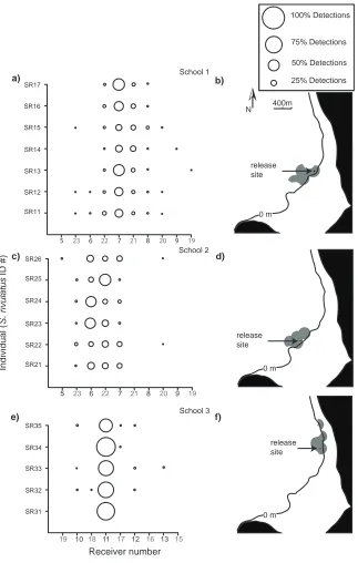
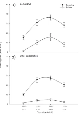
(17) Fig. 2.3 Diel detection frequency (mean detections per hourly bin over the 7-day test period ± SE) across the entire array for the two test transmitters. Shading indicates nocturnal hours (1801-0600 h).. 24. Fig. 3.1 Map of the placement of acoustic receivers (VR2W) within Pioneer Bay on Orpheus Island, Great Barrier Reef. Dark grey boxes represent the placement of shallow water receivers on the sub-tidal reef crest, and light grey boxes represent deep water receivers moored on the reef base. The circles around each receiver represent the receiver’s estimated detection range.. 37. Fig. 3.2 Plot representing the relative proportion of total diurnal detections for each individual Scarus rivulatus at each receiver for individuals in a) school 1, c) school 2 and e) school 3. The diameter of each circle is in proportion to the number of detections at a receiver. Circles provided in the legend box are examples only. Receiver numbers in black represent reef crest receivers and those in bold represent receivers on the reef base. The maximum area of reef occupied by b) school 1, d) school 2 and f) school 3 within Pioneer Bay are represented by grey areas. The solid black line represents the reef crest and the site of capture and release of the school is represented by the black dot. Only receivers with > 5% of individuals or schools detections are shown.. 44. Fig. 3.3 Frequency histogram of the average school size that individual Scarus rivulatus were associated with over a 5-min observational period (n = 60). The dashed line approximates the school size frequencies that are expected following a Poisson distribution.. 47. Fig. 3.4 Feeding rate (bites min-1; mean ± SE) of a) Scarus rivulatus and b) other scarids (which include S. ghobban, S. Schlegeli, S. niger, S. flavipectoralis and Hipposcarus longiceps) recorded for both schooling and solitary individuals at four discrete periods of the day at Pioneer Bay, Orpheus Island, Great Barrier Reef.. 48. Fig. 3.5 Conceptual model of the degradation in the feeding rate of schooling individuals as individuals’ density declines and areas of home range overlap decrease relative to non-schooling individuals, based on a doubling of feeding rates in schools. Home range overlap was created using the random allocation of five home ranges to a fixed area.. xiv. 57.

(18) Fig. 4.1 Relationship between body mass (g) and home range size (m2) for Scarus frenatus, S. niger and Chlorurus sordidus. Triangles represent juvenile individuals and squares and circles represent initial phase and terminal phase individuals respectively. Grey triangles indicate juveniles, which are predominantly omnivores/carnivores (following Bellwood 1988). The dotted vertical line indicates the maximum body mass achieved before S. frenatus and S. niger undergo juvenile to adult colour changes, and C. sordidus shifts from solitary to schooling behaviour.. 66. Fig. 4.2 Scale-independent relationship between body mass and home range size. To remove the effects of scale, body mass was cube-root transformed and home range areas were square-root transformed. Data are presented for all species; Scarus frenatus, S. niger and Chlorurus sordidus, with the dotted line representing the size at maturity. The fitted line is a logarithmic regression, see text for details.. 67. Fig. 5.1 Orpheus Island receiver (VR2W, Vemco) deployment sites. Black circles mark the location of each receiver. Filled in circles represent receivers with > 5% of at least one individual Kyphosus vaigiensis’ detections; open circles had no significant detections. a) Map of Australia showing the location of Orpheus Island along the Queensland coast. b) Array in Pioneer Bay showing depth contours and numbered stars representing capture and release sites of individuals (capture site 1: K40, K41, K42, K43, K44; capture site 2: K31, K32, K35; capture site 3: K36, K37, K38, K39; capture site 4: K33, K34). Dotted lines represent reef area.. 80. Fig. 5.2 Relationship between home range length (m) and fish body length (√fork length; mm) for carnivorous and herbivorous taxa with 95% confidence intervals for each trendline. Species with a Cook’s distance value of > 0.5 are labelled and have solid circles.. 87. Fig. 6.1 Visual representation of the simulated macroalgal outbreak depicting initial macroalgal deployment density with acoustic receiver placement.. 98. Fig. 6.2 The average abundance of a) total herbivore community and b) browsing herbivore community before (white), during (black) and after (grey) a simulated phase shift to macroalgae.. 107. xv.

(19) Fig. 6.3 Size frequency distribution of key browsing taxa; Kyphosus vaigiensis, Naso unicornis, K. cinerascens and Siganus doliatus before (white), during (black) and following (grey) a simulated phase shift to macroalgae.. 108. Fig. 6.4 Non-metric multidimensional scaling (nMDS) analysis showing the relationship between 8 sites at three different treatment levels (pre, during and post algal treatment) based on the abundance of herbivorous fish taxa. During algal deployment, sites are designated as either control or treatment. Ellipses represent significant groupings identified by ANOSIM. Vector lengths indicate the relative contribution of each species to the observed pattern. Grey triangles () represent control sites while algae were present, inverted black triangles () represent treatment sites while algae were present, unfilled triangles () represent all sites prior to algal treatment and black triangles () represent all sites postalgal treatment. 2D stress: 0.18.. 110. Fig. 6.5 Change in individual detections rates (# detections.day-1 during algal deployment - detections.day-1 prior to deployment) for all Signaus vulpinus (n = 6), S. corallinus (n = 6), Scarus schlegeli (n = 17) and Naso unicornis (n = 3). Dark grey boxes represent fishes with core areas of detection was at the algal deployment site (n = 4, 6, 9 and 3 respectively). Box represents mean ± SE and whiskers represent minimum and maximum values. None of the species’ change in detection rates following algal deployment were significantly different from zero.. xvi. 111.

(20) List of Tables Page Table 3.1 Summary of detection data and characteristics from 18 tagged Scarus rivulatus from three separate schools captured in Pioneer Bay, Orpheus Island, Australia.. 45. Table 3.2 Three-way ANOVA comparing the a) rank-transformed feeding rates for Scarus rivulatus, b) pooled log-transformed feeding rates for Scarus ghobban, Scarus schegeli, Scarus niger, Scarus flavipectoralis and Hipposcarus longiceps. 49. Table 5.1 Average metrics of Kyphosus vaigiensis movement data separated by diurnal and nocturnal sampling periods. For individual data, please see Appendix C.. 84. xvii.

(21)

(22) Chapter 1: General Introduction. Habitat modification and degradation is occurring at an unprecedented global scale, with numerous ecological repercussions (Pandolfi et al. 2003; Hoegh-Guldberg et al. 2007; Reyer et al. 2013). The human population is expected to reach 9.3 billion by 2050 (Lee 2011) and thus, an increase in the environmental disturbances caused by anthropogenic activity is inevitable (Hughes 1994; Bellwood et al. 2012; Cinner et al. 2012). Acting in concert with direct stressors, indirect impacts such as global climate change are predicted to lead to disturbance events, such as hurricanes and cyclones, of increased severity, furthering the likelihood of ecosystem degradation (Hoegh-Guldberg et al. 2007; Bell et al. 2013; Holland and Bruyère 2013). The capacity of an environment to absorb the effects of deleterious events, and return to a healthy, predisturbance state is described as that environment’s resilience (Hughes et al. 2003, 2005; Dudgeon et al. 2010). However, the resilience of the environment is largely contingent on several factors that can undermine or support it. Chronic pressures are among the most significant contributors to reduced resilience (Nyström et al. 2008; Hughes et al. 2010). Examples of chronic environmental disturbances include introduced species (Vitousek et al. 1997), nutrient loading and eutrophication (Smith and Schindler 2009) and overexploitation of natural populations (Lokrantz et al. 2010). Probably the best example of the effects of multiple chronic pressures on coral reefs has been reported from the Caribbean. Overfishing reduced the resilience of Caribbean coral reefs by significantly reducing piscine herbivore populations, reducing ecological redundancies (Jackson et al. 2001; Knowlton 2001; Hughes et al. 2003). As a result, the environment was unable to recover to a pre-disturbance state following the regional scale loss of Diadema. 1.

(23) antillarum and a range of other local stresses. This produced a large-scale phase-shift that occurred on Jamaican reefs (Hughes et al. 1994). This phase-shift resulted in the reef community shifting away from a coral dominated state, to one in which macroalgae covered the majority of the benthos (Hughes et al. 1994; Connell 1997). Since then, experimental studies have been able to simulate a similar effect on other tropical reefs by excluding key species and simulating a scenario where a system’s resilience has been undermined (e.g. Stephenson and Searles 1960; Hughes et al. 2007; Burkepile and Hay 2010). Thus, we know how declines in coral reef health are triggered. The challenge now is to prevent ecosystem decline by identifying and managing ecological processes that support ecosystem resilience. Among the key elements in ecosystem resilience are the interactions between taxa and their environments (Bellwood et al. 2004; Elmqvist et al. 2010). Ecosystems are reliant on a variety of functions provided by several taxa, which maintain the environment in a normal, healthy state (Bellwood et al. 2004; Carpenter et al. 2006; Olds et al. 2012). Examples of such functions include predation, essential for maintaining stable, diverse populations (Terborgh et al. 2001; Knight et al. 2005); detritivory, facilitating nutrient cycling (Depczynski and Bellwood 2003); and herbivory, which controls algal communities (Ledlie et al. 2007; Burkepile and Hay 2010). While the functions are numerous, the species responsible for each function can be few in number and vary extensively over different spatial scales (Cheal et al. 2012). Functional redundancy has been suggested to be an essential element of ecological resilience, in that key functional roles can be fulfilled by various species, providing insurance for ecosystem functions (Sundstrom et al. 2012). However, recent evidence suggests that functional redundancy is not as prevalent as previously assumed (Bellwood et al. 2006; Brandl and Bellwood 2013; Johansson et al. 2013). Due to the fine-scale niche partitioning that can exist in complex biological systems (a. 2.

(24) characteristic of the tropics), there are often limited numbers of taxa capable of conferring essential ecosystem services (Connell 1997; Patterson et al. 2003; Fox and Bellwood 2013; Mouillot et al. 2013). Coral reefs are among the best examples, with herbivorous coral reef fish being among the most important for reef resilience (e.g. Hughes et al 2007). Within the herbivores, several contrasting functions exist and each is dominated by a limited number of taxa (Bellwood et al. 2004; Burkepile and Hay 2008; Hoey and Bellwood 2009). Furthermore, when assessed using bioassays and manipulative experiments, the rates at which the functional processes are applied and the primary species driving them are highly variable at a range of spatial scales (Bennett and Bellwood 2011; Vergés et al. 2011; Johansson et al. 2013). The spatial scales over which functions are applied, is inherently bound by the home ranges of those that moderate the process. In this sense, a great deal of the observed variability in functional processes on coral reefs may result from the spatial biology of key taxa (Fox and Bellwood 2011; Welsh and Bellwood 2012a). Traditionally, the home ranges of animals have been assessed to estimate the effectiveness of protected areas (e.g. Meyer and Holland 2005; Afonso et al. 2009; Bryars et al. 2012), or nature reserves (e.g. Eloff 1959; Broomhall et al. 2003), and to understand migration pathways of charismatic or commercially important species (e.g. Berger 2004; Hedger et al. 2008). However, few studies have considered the importance of interactions between organisms and their environment, in the context of home ranges (but see Cooke et al. 2004; Owen-Smith et al. 2010; Fox and Bellwood 2011; Welsh and Bellwood 2012a). It is surprising that a factor such as movement, which is intrinsic to the application of functional process, has been largely overlooked on coral reefs, one of the most threatened environments. Given the logistical constraints of assessing the home ranges of fishes, spatial studies in the marine environment have historically lagged behind their terrestrial. 3.

(25) counterparts. The methods associated with quantifying movement in terrestrial systems have evolved over time from visual observations and mapping, to radio telemetry (Harris et al. 1990; Laver & Kelly 2008) and satellite tagging (Jouventin & Weimerskirch 1990). In the case of marine species, especially fishes, before the late 90s studies were largely restricted to visual observations (Kramer & Chapman 1999), due to the limitations of working in the marine environment (but see Holland et al. 1996; Zeller 1997). However the application and refinement of acoustic telemetry in the last few decades has made it possible to accurately monitor the movement of marine species and to estimate the home range of a broader range of taxa (Fig.1.1; Bolden 2001;. Number of studies. Voegeli et al. 2001; Cooke et al. 2004; Heupel et al. 2006).. 40 30. Visual Telemetry Other. 20 10 0 1984− 1994− 2004− 1993 2003 2013. Fig. 1.1 Number of studies evaluating the home range size in reef fishes using visual estimations, acoustic telemetry (active and passive combined) and other methods (Modified from Nash et al. in review).. 4.

(26) The evolution of acoustic telemetry as a means to monitor the movement of marine taxa has largely evolved in two directions; active and passive acoustic monitoring. Active acoustic monitoring is used to collect high-resolution data on the short-term movements of a focal individual (Meyer and Holland 2005; Fox and Bellwood 2011; Welsh and Bellwood 2012a). While this technique is useful for studies that require highly detailed data on animal movements, it is limited in that the battery life of the transmitters is often less than a month, data collection is labour intensive (Voegeli et al. 2001) and tracking fish from motorized vessels in shallow water may modify their behavior (Meyer and Holland 2005; Welsh and Bellwood 2012a). For long-term studies, passive acoustic monitoring is often favoured. Using passive acoustic monitoring, the presence or absence data of many tagged individuals can be collected by a network of acoustic receivers for a period of months to years (Fig. 1.2a, b; Heupel et al. 2006; Welsh et al. 2012). Another benefit of this technology is that movements can be tracked over large spatial scales with minimal upkeep and maintenance of the receivers (Heupel et al. 2008). Therefore, data can be continuously collected, even in remote location when continued access to field sites may not be permitted. With the development of these tracking techniques for the marine environment, the study of coral reef fish spatial biology has represented a burgeoning field of research. However, the application of animal movement data to ecological questions has been limited and thus, our understanding of the ecological implications of reef fish movement remain in its infancy. The aim of this thesis, therefore, is to provide a spatial context for ecological interactions and to evaluate for the importance of spatial biology in ecological research. More specifically, the studies herein are aimed to place the ecosystem functions of key. 5.

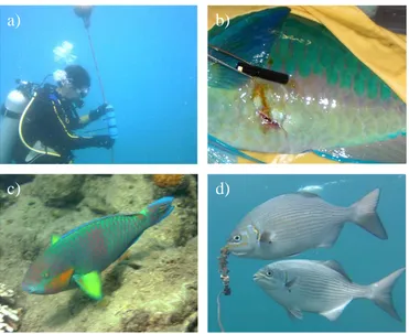
(27) herbivorous fish taxa on the Great Barrier Reef (GBR) in a spatial context and to assess to what extent their movement patterns may influence ecosystem resilience.. a). b). c). d). Fig. 1.2 a) VR2W acoustic receiver mooring b) acoustic transmitter implanted into visceral cavity c) study species used in Chapter 2, Scarus rivulatus and d) study species used in Chapter 5, Kyphosus vaigiensis.. We address the objective of the thesis in five data chapters. Each data chapter either relates to a publication derived from the present work or has been submitted for review in a scientific journal (Appendix F). The evaluation of spatial patterns in reef fishes are limited, especially when compared to terrestrial taxa or even temperate or pelagic fishes. This is partially a result of the difficulties in collecting telemetry data for coral reef species, even using modern acoustic telemetry. Therefore, the question remains as to how acoustic receivers perform on coral reefs and whether or not they can 6.

(28) be used as an effective tool to quantify the movements of benthic fish taxa. In Chapter 2 this question is addressed, with an evaluation of the performance of ultrasonic acoustic receivers on coral reefs (Fig. 1.1a, b). Furthermore, this chapter provides data to inform the construction of acoustic arrays and information pertaining to the interpretation of animal movement patterns derived from acoustic telemetry on coral reefs. With methods established to monitor the movements of fishes on coral reefs using acoustic telemetry, questions regarding the scale of movements, and thus ecological interactions, conferred by key taxa can be addressed. Chapter 3 evaluates the link between social systems and home range extent in parrotfishes. This question is addressed by quantifying the movement patterns of Scarus rivulatus (Fig. 1.1c), an important reef herbivore on the GBR, and their foraging schools, placing the term ‘roving herbivore’ in a spatial context. In Chapter 4 the rate of ontogenetic home range expansion is assessed for a number of different parrotfish species as they grow in body mass over five orders of magnitude. The resulting pattern is then compared to that of higher vertebrates. Despite a growing body of literature on the movements of coral reef fishes, the true maximum of mobility in herbivorous coral reef fishes is yet to be assessed, and the key question of ‘what is a true roving herbivore’ remains. Chapter 5 assesses the movements of a browsing herbivore Kyphosus vaigiensis (Fig. 1.1d) over large spatial scales to address this question. The movements of this species were then compared to all available studies conducted on reef fishes in order to create a context by which large-scale movements can be identified. Finally, Chapter 6 presents a manipulative experiment in which habitat degradation is simulated on a coral reef and the spatial response of resident and nonresident coral reef herbivores is assessed. This thesis is ends with a concluding discussion which examines the importance of the spatial biology of reef fishes in. 7.

(29) relation to ecosystem functioning and provides a summary of the studies available on the movements of coral reef fishes.. 8.

(30) Chapter 2: Performance of remote acoustic receivers within a coral reef habitat: implications for array design Published in Coral Reefs 2012 31: 693-702. 2.1. Introduction Investigations of the movement patterns and site fidelity of aquatic species are now increasingly being carried out using passive (remote) acoustic monitoring, where focal individuals are tagged with coded transmitters and are monitored at automated listening stations (receivers) (Afonso et al. 2009; Semmens et al. 2010; Simpfendorfer et al. 2011). Of all peer-reviewed studies carried out using remote acoustic telemetry, more than one-third have been published in the last 3 years. Passive acoustic monitoring, therefore, represents a burgeoning field, presenting the opportunity to track the movement of individuals over periods of months (Egli and Babcock 2004; March et al. 2010) or years (Afonso et al. 2008; Meyer et al. 2010), and giving researchers the opportunity to test hypotheses relating to long-term habitat usage and site fidelity. The technology has been most frequently employed within estuarine (e.g. Hartill et al. 2003; Heupel et al. 2006), riverine (e.g. Winter et al. 2006) or deep-water oceanic habitats (e.g. Clements et al. 2005). Increasingly, however, the methodology is being utilized within the coral reef environment, particularly to answer important questions relating to the site fidelity and habitat use of harvested reef fish species (e.g. Meyer et al. 2010; O’Toole et al. 2011). Despite the remarkable technological advances that have facilitated the increased ease and flexibility of use of remote acoustic monitoring, the interpretation of data collected by automated listening stations is still a developing area of research (Lacroix and Voegeli 2000; Clements et al. 2005; Simpfendorfer et al. 2008). Critical to the. 9.

(31) interpretation of detections made by an acoustic array is an understanding of both the detection range (Klimley et al. 1998) and the performance (sensu Simpfendorfer et al. 2008) of receivers within that array. Ultimately, the coverage yielded by the array at any given time will determine whether the data collected represents either a minimum or complete estimate of the animal’s movement range. Detection ranges are all too frequently assumed, rather than tested. Where range tests are undertaken and reported for individual studies, detection ranges can deviate from the value reported in manufacturers’ product specifications, highlighting the discrepancy in listening range for receivers within different aquatic habitats (Voegeli and Pincock 1996; Heupel et al. 2006). Both the detection range and performance of individual monitoring stations have been shown to be highly variable on temporal and spatial scales (Simpfendorfer et al. 2008; Payne et al. 2010). Without a full understanding of this variability in performance, the behaviour of the organisms being studied can be grossly misinterpreted (e.g. Payne et al. 2010). The constraints of the technology, and the potential for variability in the detection performance of monitoring stations highlights the importance of properly evaluating receiver performance prior to and during each individual study (Heupel et al. 2006). However, there is currently a paucity of studies focusing on the acoustic equipment and its performance, especially on coral reefs (Heupel et al. 2008). As information on equipment performance in any given environment is integral to understanding telemetry results, variability in detection ranges between different environments should be a consideration in data analysis and interpretation. This is particularly important on coral reefs, which represent a relatively new and potentially difficult environment for the acoustic technology. Coral reefs are extremely noisy environments with a plethora of reef noise generated by the feeding, mating and territorial displays of invertebrates and fish taxa (e.g. Cato 1978; McCauley and Cato 2000; Simpson et al. 2008a, b). Reef. 10.

(32) noise, coupled with the high topographic complexity of coral reefs, may result in a highly variable acoustic receiver detection range, unique to the reef environment. The synergistic effects of the aforementioned obstacles when working on coral reefs stand to significantly affect the performance of acoustic receivers, with median detection ranges being reported as low as 108 m with a minimum value of 55 m (Meyer et al. 2010), well below manufacturer’s specifications. Recently, several performance metrics such as code detection efficiency, rejection coefficients, and noise quotients have become available, making it possible to evaluate the performance of receivers individually. The availability of performance metrics at the scale of the individual receiver has created the potential to better understand how the complexity and acoustic environment of coral reefs are influencing the receiver’s capacity to detect acoustic transmitters, ultimately leading to an ameliorated capacity to interpret telemetry data (Simpfendorfer et al. 2008). The goals of the current study were: first, to investigate the detection range and performance of ultrasonic acoustic receivers within a specific shallow coral reef environment and, second, to provide data to inform the design of listening arrays and interpretation of animal movement patterns within coral reef habitats more generally. The specific aims of the study were to determine (1) the effective working detection range of 9-mm acoustic transmitters within a coral reef environment, and (2) the extent of diel variability in acoustic receiver performance on a coral reef.. 2.2. Materials and Methods The study site was a 1.5-km stretch of fringing reef within Pioneer Bay, Orpheus Island, a granitic island in the inner-shelf region of the Great Barrier Reef lagoon (Fig. 2.1a). The leeward stretch of reef within Pioneer Bay is a low-energy environment composed. 11.

(33) of an extensive reef flat that reaches up to 400 m from the shoreline (details in Fox and Bellwood 2007). The reef flat has little topographic complexity and is frequently exposed at low tide. The reef crest is not sharply defined and is composed of many bare patches of consolidated substratum. The crest gives way to a gentle slope that displays high topographic complexity in many places near the crest created by large colonies of Porites spp. and Acropora spp. interspersed with sand and coral rubble areas, which create gullies and channels in many areas. At a depth of approximately 5 m (below chart datum) the topographic complexity decreases and the reef slope continues as a gently sloping sand substratum with occasional low patches of coral before flattening off at approximately 18 m. Due to its location on the inner part of the continental shelf and proximity to the mouth of the Herbert River, the reef on the leeward side of Orpheus Island is in a high sediment environment, with turbidity often resulting in visibility dropping to less than 2 m. Visibility is usually in the region of 4-10 m. Water turbidity was consistent throughout the study period, with visibility remaining at approximately 3 m.. 12.

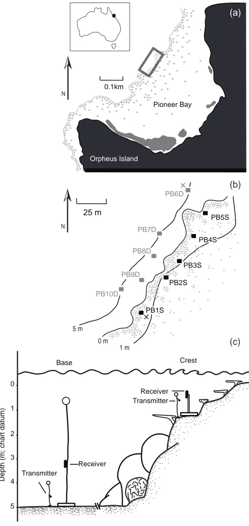
(34) (a). 0.1km N. Pioneer Bay. Orpheus Island. (b) PB6D. 25 m. PB5S. N. PB7D PB4S PB8D PB3S PB9D PB2S PB10D PB1S 5m. (c). 0m 1m Crest. Base 0. Depth (m; chart datum). Receiver Transmitter 1. 2 3 Receiver Transmitter 4. 5. Fig. 2.1 Study site. Pioneer Bay, Orpheus Island, Great Barrier Reef. a) Map showing location of range testing array within Pioneer Bay, b) locations of remote acoustic receivers along reef base contour (grey squares) and reef crest contour (black squares), fixed delay test transmitters (Vemco, V9-1L) were moored 0.5 m above the substratum at opposite ends of the array at deep (grey cross) and shallow (black cross) positions, and c) an illustration of the depth at which the receivers were placed as well as the reef profile (please note, receivers and transmitters are not to scale, horizontal axis is truncated; receivers are 25 m apart). 13.

(35) Transmitter detection-range tests. Maximum detection range. Prior to the commencement of the study, preliminary tests were carried out to determine the maximum unobstructed detection range of 9-mm acoustic transmitters using fixed delay transmitters, which have a predictable, and constant, transmission interval (Vemco, V9-1L, 69 kHz, 5-s repeat rate, power output 146 dB re 1 lPa at 1 m). These data were then used to estimate effective distance increments between receivers for temporal detection range evaluations. In these initial tests, a single remote acoustic receiver (VR2W, Vemco. Ltd., NS, Canada) was moored at a depth of 2 m (approximately 5 m seaward off the reef crest). A fixed delay transmitter was then moored for approximately 15 min at a distance of 50 m from the receiver, a sufficient amount of time for the transmitter to produce more than 100 signal transmissions. After this time, the transmitter was moved parallel to the reef, maintaining the same depth, to a distance of 75 m where it was moored for an additional 15 min. The procedure was repeated at 100, 125 and 150 m fixed distances from the receiver. The detection efficiency of the receiver at each distance was then calculated based on the number of recorded detections divided by the number expected over the deployment period at each distance increment. The value for the expected number of detections could be calculated from preliminary laboratory tests of the transmitter run prior to the field deployment, as signals were produced by the transmitter at fixed, non-random time intervals. The transmission interval was determined to be 8 s as a result of the approximate 3 s it takes for the transmitter to emit a complete signal pulse train coupled with the 5-s fixed delay transmission interval, giving an expected detection rate of 7.5 signals min-1.. 14.

(36) Effective detection range and temporal variation in detection. Between 25th February and 3rd March 2011, 10 VR2W acoustic receivers were deployed in Pioneer Bay. Based on the results of preliminary tests to determine maximum detection range within the reef habitat (see above), the receivers were positioned in parallel lines following two distinct reef zones. Each line along the reef consisted of 5 VR2W receivers and was configured with the first two receivers spaced 50 m apart and the remaining 3 receivers spaced at 25 m increments (i.e. 0, 50, 75, 100 and 125 m from start point respectively; Fig. 2.1b). This deployment configuration is designed to achieve high detection area coverage to estimate various spatial attributes of site attached fish such as their home range (e.g. Marshell et al. 2011) or the median distance travelled (Murchie et al. 2010). One line of receivers was positioned just shoreward of the reef crest while the other receiver line followed the reef base contour (Fig. 2.1b). Moorings for the receivers on the reef crest were placed at a depth of approximately 1 m (below chart datum) and consisted of a 50 cm metal pole, the base of which was sunk into a 30 kg concrete block. Receivers were fixed to the pole and oriented vertically upwards with the hydrophone extending 10 cm above the top of the metal pole in order to minimise interference between the mooring structure and hydrophone reception (Clements et al. 2005). The shallow crest receivers were therefore about 0.5 m below chart datum. Receivers along the reef base contour were attached to a simple rope mooring which was anchored to the sea floor at a depth of approximately 5 m. Receivers were fixed to the rope at least 1 m below a sub-surface float, which held the receiver vertical in the water column at a depth of about 3 m. While the receivers were deployed, climactic conditions remained consistent, with moderate winds (< 15 kn) and swell (< 60 cm), overcast skies and < 1 mm of rain.. 15.

(37) Two coded transmitters (Vemco, V9-1L, 69 kHz, random delay interval 190-290 s, power output 146 dB re 1 µPa at 1m) were moored at opposite ends of each receiver line, one adjacent to receiver PB1 (1 m from receiver; transmitter 1) and the other adjacent to receiver PB6 (transmitter 2) (Fig. 2.1b, c). The transmitters were held 0.5 m from the substratum, simulating the depth at which most medium to large (20-70 cm TL) benthic reef fish would be active while foraging or swimming. As a result of the long random delay interval of the transmitters used in the long-term range testing experiment, the number of code transmissions produced cannot be calculated with the required precision over short time periods (hours) in the same manner as a transmitter with a fixed delay transmission interval. Therefore, the number of detections recorded by PB1 and PB6 for transmitters 1 and 2, respectively, were used for analysis as the number of transmissions made by each transmitter during the study period. The transmitters were left in place for a 7 d period, after which time they were removed from the study site and the detection data files downloaded from each VR2W receiver. Immediately after the 7-day data collection period, the transmitters used for the longterm deployment were assessed to determine if they were representative of typical V9 transmitters. To do this, both transmitters used in the study and an identical third transmitter (Vemco, V9-1L, 69 kHz, random delay interval 190-290 s, power output 146 dB re 1 µPa at 1m) were moved to a mooring 50 m from a receiver, which was left in place for a 12 h period. Following this, the receiver was collected and data was downloaded to compare the average number of detections from each transmitter during five randomly selected 30 min time periods.. 16.

(38) Data analysis. Overall detection probabilities and effective detection range. The average number of detections from the transmitters deployed on the array, and a third transmitter, were compared using a one-way ANOVA. The assumption of normality was inspected using residual plots, and homogeneity of variances was checked using Levene’s test for homogeneity of variances. No transformations were required to meet the assumptions of ANOVA. For each of the two test transmitters, detections recorded at individual receivers over the 7-day test period were grouped into 6-h bins and classified as either ‘‘day’’ (0601-1800 hours) or ‘‘night’’ (1801-0600 hours). Individual detection probabilities for each 6-h period at each receiver were calculated based on the total number of recorded detections expressed as a percentage of the known number of transmissions (derived from the number of detections from the receiver adjacent to the transmitter). Missed transmissions due to signal overlap from occasional visits of tagged taxa to the study site were factored into the analysis. Individual detection probabilities for each receiver were then plotted against the distance from the receiver to the transmitter for diurnal and nocturnal sampling periods. Detections were modeled using linear regressions and logistic regressions. For the reef base, a linear regression analysis was the best model for the data (distance to transmitter as independent variable). For the reef crest, the relationship between number of detections (number of signals per day present vs. absent across the array) and the distance from the transmitter was best modeled by a logistic regression.. 17.

(39) Temporal (diel) variation in detection. Temporal variation in detection probabilities were examined by calculating the average number of detections for each of the 12-h diurnal and nocturnal sampling periods (average values per 12-h bin were treated as individual data points for analysis). Differences in the proportion of signals detected by each receiver in diurnal and nocturnal sampling periods were then compared using a repeated measures analysis of variance (RMANOVA). To evaluate the effect of interference, which may occur on a regular diel basis (such as reef noise), diel detection densities (hourly detection frequencies) across the array as a whole were also examined. For each day during which the array was in place, detections from the two test transmitters were grouped into hourly bins to give a total number of detections hour-1 by the array. Hourly values were then averaged across the 7 days of the study to give a mean hourly detection frequency in each of the 24 hourly bins, and these hourly detection frequencies were compared using a Chi-squared goodness of fit test. To detect any fine-scale cyclical patterns in diel detection frequency, a Fast Fourier Transformation (FFT) (with Hamming window smoothing) was also applied to the data. Following Payne et al. (2010) the magnitude of variation of each hourly bin (the standardized detection frequency or SDF) around the overall mean daily detection frequency was then calculated as: SDFb = Bb/µ, where B is the mean detection frequency in each of the hourly bins and l is the overall mean detection frequency. Therefore, should acoustic interference be high at certain periods of the day, we would expect low SDF values for the hourly bins during that time period as the receiver would be detecting fewer than average detections. This provides an indication of the extent to which transmitter detections may have been under-represented during particular parts of the diel cycle due to environmental factors.. 18.

(40) Acoustic performance. Parameters recorded in the metadata file downloaded from each VR2W receiver were used to provide a quantitative metrics of the overall performance of the array. Metrics were based around four specific parameters relating to the 8-pulse train emitted by the coded transmitters used in this study: (1) the total number of pulses recorded each day by a receiver (P); (2) the number of recorded detections (D); (3) the number of valid synchs (where a synch is the interval between the first two pulses of the 8-pulse train that identifies the incoming code as belonging to a transmitter) (S) and; (4) the number of codes rejected due to invalid checksum periods between the final two pulses of the train (C). From these parameters the daily code detection efficiency (D!S-1), daily rejection coefficient (C!S-1) and daily noise quotient (P-S!# of pulses required to make a valid code) were calculated for each receiver (see Simpfendorfer et al. 2008 for further description of individual parameters and metrics). It is worth noting that the VR2W can also count non-synch periods (periods generated by transmission overlap and noise interpreted by the receiver as pings) as syncs, however, there was very little evidence of this factor herein. The effect of the receiver’s distance from each of the moored transmitters on the aforementioned performance metrics was evaluated using Pearson’s correlation analysis.. 2.3 Results Maximum detection range. The preliminary tests of maximum detection range revealed a rapid decline in detection probability for a 9 mm transmitter over short distances within the reef environment. At 50 m from the receiver only 62% of transmissions from a fixed delay range-testing. 19.

(41) transmitter were detected, decreasing to a probability of just 4% at a distance of 150 m. At a distance of 125 m from the receiver, 22% of transmissions were detected, beyond this distance, detection values fell to below 5% and therefore, 125 m was taken to be the maximum workable detection range within the study reef environment. This means that, in the absence of other competing transmitters, a lone individual tagged with an acoustic transmitter must be resident, on average, for at least 1090 s ([190 + 290]!0.22-1) to be detected at a distance of 125m.. Overall detection probabilities and detection range. For each transmitter a significant negative relationship existed between both diurnal and nocturnal detection probabilities and distance from receiver (Fig. 2.2). The slopes and intercepts for the regression equations for diurnal and nocturnal periods were similar on both the reef crest (y = e4.91-0.08(x)/(1 + e4.91-0.08(x) and y = e4.75-0.07(x)/(1 + e4.91-0.08(x), respectively) and on the base (y = 94.56-0.52x and y = 90.92-0.49x, respectively). For the 9-mm transmitter (random delay interval transmitter) moored on the reef base (next to the deep receiver line), detection probabilities decreased gradually at increasing distance from the receiver (Fig. 2.2a). For practical purposes, a cut-off of 50% detection efficiency was deemed acceptable for biological interpretation (Payne et al. 2010), meaning that the effective working detection range for this deep transmitter was 90 m. However, an average 30% of detections were still being recorded at a distance of 125 m from the transmitter. For the 9-mm transmitter moored on the reef crest (next to the shallow receiver line), detections dropped off much more steeply, driven for the most part by the small probability of detection by receivers moored along the reef base (Fig. 2.2b). In this case, the working (50%) detection range was just 60 m (Fig. 2.2b), although this increased to approximately 90 m when considering only detections by the. 20.

(42) shallow line of receivers. In contrast to the results for the deep transmitter, virtually no detections were being recorded at a distance of 125 m from the shallow transmitter, even by the shallow line of receivers (Fig. 2.2b). Differences in the number of detections from the transmitter deployed on the reef base and the one on the reef crest cannot be attributed to differences in transmitter performance. Post hoc tests revealed no significant difference between the numbers of transmissions made by either of the transmitters used over the 7-day trial period or a third transmitter used to compare transmitter performance (F2,12 = 1.27, P > 0.05).. 21.

(43) PB6D. PB5S. 100. (a) Reef base transmitter. PB4S. PB3S PB7D. 80. PB8D. PB10D. PB2S PB9D. 60. PB1S. Probability of detection (%). 40. Day Night. 20. 0 0. 20. 40. 60. 80. PB9D PB10D PB2S. 100. 100. 120. 140. (b) Reef crest transmitter PB3S. 80. PB1S PB8D. PB4S. 60. 40. 20. PB7D PB5S. 0 0. 20. 40. 60. 80. 100. 120. 140. Distance to transmitter (m). Fig. 2.2 a) Relationship between the probability of detection and distance from the receiver for a transmitter moored on the reef base during diurnal hours (grey line, linear regression, slope = -0.52, constant = 94.56, P < 0.001, r2 = 0.52) and nocturnal hours (black line, linear regression, slope = -0.49, constant = 90.92, P < 0.001, r2 = 0.48) and b) relationship between the number of successful versus unsuccessful detections and distance from the receiver for a transmitter moored on the reef crest during diurnal hours (grey line, logistic regression, slope = -0.084, constant = 2.35, P < 0.001, Nagelkerke r2 = 0.71) and nocturnal hours (black line, logistic regression, slope = 0.067, constant = 4.08, P < 0.001, Nagelkerke r2 = 0.64). Detection probabilities are shown for each 6-h period of the 7-day test and are classified as diurnal (0601-1800 h) (grey circles) or nocturnal (1801-0600 h) (black circles). Nocturnal data points have been shifted slightly left on the y-axis to eliminated significant overlap with diurnal data points.. 22.

(44) Temporal (diel) variation in detection. The comparison of average detection probabilities for 12-h diurnal and nocturnal periods revealed no significant diel difference in signal detection probability for the deep receiver line (F1,8 = 0.17, P = 0.69) or the shallow receiver line (F1,8 = 0.02, P = 0.88). On an hour-by-hour basis there were some differences in detection frequencies over the course of the day (χ222 = 34.62, P = 0.042). However, the overall diel pattern of detection densities did not reveal any distinct trend in over- or under-representation of detections during nocturnal or diurnal hours (Fig. 2.3). FFT analysis likewise revealed no prominent diel cycles of detection in the observed power spectrum (please see Appendix A for FFT output). Instead, several major peaks were found and those with the greatest spectral density occurred at 40, 10 and 16.7 hour cycles (see Appendix A). Standardisation of detection frequencies to remove any artefacts of environment and varying distance to receiver on detection frequency confirmed that there was little diel variation in detection density, with the only discernable pattern being an underrepresentation of detections in the period around dawn (0500-0600 h) (Fig. 2.3). Otherwise, both positive and negative variation around the mean daily detection frequency was observed in both diurnal and nocturnal periods (Fig. 2.3).. 23.

(45) Mean detection frequency -1 (detections h ± SE). 180 160 140 120 100 80 60. 0. 6. 12. 18. 23. Hourly bin. Fig. 2.3 Diel detection frequency (mean detections per hourly bin over the 7-day test period ± SE) across the entire array for the two test transmitters. Shading indicates nocturnal hours (1801-0600 h).. Receiver Performance. The daily code detection efficiency of the receivers used in this study ranged from 0.27 to 0.82 detections synch-1, with an overall average of 0.52 detections synch-1 (± 0.01 SE). This meant that just over half the codes transmitted by the two transmitters were successfully recorded by the receiver array. The mean rate of code rejection was just 0.022 (± 0.001), suggesting that, on average, only 2% of codes were rejected due to invalid checksum periods. The value of the noise quotient recorded by each receiver was almost universally negative in value and averaged -1,067.8 (± 87.5). There was no relationship between the distance of receivers to transmitters and code detection. 24.

(46) efficiency (r = -0.20, P > 0.05), code rejection rate (r = 0.23, P > 0.05) or the noise quotient (r = -0.16, P > 0.05).. 2.4 Discussion Our results suggest that the working detection range for 9-mm transmitters (Vemco, V9-1L, 69 kHz, power output 146 dB re 1 µPa at 1m), the size most suited for the majority of benthic reef fishes on coral reefs, may be as low as 60 m. While transmitters with higher power outputs may be detectable at a slightly greater range, this value is a fraction of the ranges previously reported in the literature for this size of transmitter within aquatic habitats. For example, a 450-m range was reported for 9-mm transmitters in the Caloosahatchee River (Simpfendorfer et al. 2008), and a 200-m detection range was reported for V9-2L transmitters (with a similar power output to those used herein) in temperate reef habitats of South Australia (Payne et al. 2010). Instead, the overall detection range found herein is most comparable to the minimum detection range of 60 m reported by Meyer et al. (2010) on Hawaiian reefs. Our results suggest that the detection performance of acoustic receivers may be significantly impacted by the unique nature of the reef environment and demonstrates the importance of testing the range of acoustic arrays across individual habitats and study sites. In the case of Pioneer Bay, the receiver performance metrics may provide potential explanations for the reduced detection ranges reported. The low code rejection coefficients exhibited by receivers indicates that codes were not being rejected because of invalid checksum values (values that check the integrity of the code transmission used by the receiver to validate the code and confirm it is a recognisable transmitter). The reduced detection efficiencies recorded in this study, therefore, were driven by the receiver unit not receiving the full sequence of pulses emitted by the transmitter. For the coral reef environment, there are several possible explanations for the reception of 25.

(47) incomplete code sequences by the receiver. These include (1) distortion of the acoustic pulse train (e.g. dampening of amplitude) via interference from environmental noise (acoustic waves) (both physical and biological sources and periodic or chronic); (2) the distortion of the code sequence via reflection off topographically complex substrata; (3) the distortion of the code sequence via absorption by particles in the water; (4) collision with pulses from other transmitters within the detection range of the receiver; (5) blockage of the transmission by a tagged individual moving behind an obstacle. In the case of the current study, the latter two explanations can be eliminated by virtue of the fact that detection performance was based on stationary transmitters operating in an environment with minimal transmitters present. This leaves background noise, suspended sediment and topography as likely explanations for the fact that transmitter code sequences attenuated over shorter than expected distances in the reef environment. In terms of background noise, it has been suggested previously that the capacity of an acoustic receiver to detect a signal emitted by a transmitter is hindered in the presence of large amounts of background interference, such as the noise generated by snapping shrimp and other marine taxa (e.g. Voegeli and Pincock 1996; Clements et al. 2005; Simpfendorfer et al. 2008). Intermittent noise recorded as a ping during an actual transmitter’s transmission can cause the receiver to reject the transmission, resulting in the receiver ignoring the actual transmitter’s acoustic signal. Continuous noise can raise the threshold required to detect a transmission from a transmitter resulting in a lower detection range (with fewer pings likely to be detected). Reefs are notoriously noisy environments and, undeniably, there is a range of noises on coral reefs, mostly biological in origin, occurring over an extremely broad acoustic spectrum. Reef noise has been documented to reach frequencies as high as 200 kHz, in the case of the noise produced by snapping shrimp (Au and Banks 1998). The evidence from the negative noise quotient values in the present study suggests that, in the reef environment, the. 26.

(48) receivers are not hearing intermittent noise, which would contribute to a high noise quotient value, but are perhaps hearing continuous noise. Continuous background noise would cause the receivers to adjust their signal detection sensitivity to ignore consistent background noise, which may result in the occasional signal from the transmitter being ignored, thus contributing to a lower detection range than has been reported in other aquatic environments. A further manner by which ambient noise may reduce the detection capacities of the receiver is by modifying the acoustic signal of the transmitter itself. The further the acoustic signal from a transmitter must travel, the more likely it becomes that the signal will collide with other noise and thus, be modified. In this sense, reef noise may cause an incomplete pulse train to reach the receiver. Ambient noise may therefore have both an indirect (interference with the transmitter) and direct (interference with the receiver) effect on acoustic signal detection. Surprisingly, the current study did not detect a significant difference between the diurnal and nocturnal performance of acoustic receivers within the reef habitat, something which has been reported in other environments where testing of passive acoustic arrays has been undertaken (Payne et al. 2010). In temperate, shallow, marine environments and estuaries, the temporal variation in activity of invertebrates such as snapping shrimp have been suggested as the cause of these patterns in the detection range of acoustic receivers (Heupel et al. 2004, 2006). While the source of biological noise on reefs is highly variable, and possibly more intense at night (Bardyshev 2007), the acoustic characteristics of the noises produced are actually quite similar in diurnal and nocturnal periods (Leis et al. 2002). Choruses from fish schools (McCauley and Cato 2000) and invertebrates can be heard in both diurnal and nocturnal time periods (Radford et al. 2008). Therefore, should noise be capable of having a significant impact on the signal transmitted from a transmitter, it is likely to be having a similar impact in. 27.

(49) both nocturnal and diurnal sampling periods. Small, yet significant, declines in the number of detects were, however, recorded at dawn and dusk. These trends may arise as a result of an increased instance of reef noise documented to occur during these time periods on tropical reefs from fish choruses and invertebrates (Fish 1964; Cato 1978; Radford et al. 2008). However, the absence of a distinct peak in the spectral density of the FFT analysis herein suggests that these patterns are non-cyclic, and may be random noise. This is most apparent when our results are compared to the strong spectral peaks at 24 h, and secondary peaks at 6 and 12 h, described by Payne et al. (2010) using stationary control transmitters. Although we did not see the same degree of diel variation in the mean detection frequency of transmitters reported from previous studies (Payne et al. 2010), our results do suggest that, to at least some extent, background noise is contributing to lower detection ranges and small detection probabilities. Within the reef environment at Pioneer Bay, several physical factors are also likely to have contributed to interference in signal detection by physically blocking the acoustic signal. High levels of suspended matter that are characteristic of turbid inshore reefs, such as Orpheus Island, may cause reflection of acoustic signals, interrupting acoustic pulse trains (Voegeli and Pincock 1996 cited in Simpfendorfer et al. 2008). Moreover, the natural topographic complexity of reefs mean that a clear line of sight between receiver and transmitter is likely to be more frequently breached than in a sandy or muddy-bottomed lagoonal or estuarine habitat. Even in the current study where receivers were detecting stationary transmitters, high topographic complexity may have an impact on detection ability. Receiver PB7D, which consistently performed below the level expected given its distance to the two transmitters, was in close proximity to significant benthic complexity, which is likely to have effectively and consistently blocked the acoustic signal. This result, even on a stationary transmitter, stresses the importance of both optimal receiver placement and assessment of the. 28.

(50) detection performance of individual receivers to the design of an effective remote monitoring array. However, the precise causes of the strong signal attenuation are probably complex and may have several contributing factors. Intra-environmental variability in receiver detection capacities, both holistically and in terms of diel variation, as seen in temperate reefs (e.g. Payne et al. 2010), highlight the need to perform detailed range tests when utilizing acoustic telemetry to monitor movement biology. Moreover, the unique performance of acoustic telemetry in a variety of environments emphasizes the dangers of simply inferring detection ranges from previous studies. It is strongly recommended that simple range tests, such as those conducted herein, be undertaken to assess maximum detection ranges in arrays, to help avoid misinterpretation of results. Knowledge of the study environment and careful selection of individual receiver placement is imperative to inferring the detection range not only of individual receivers, but also the area covered by the detection array. Similar to the reduced detection capacity of receiver PB7D, those receivers moored on the deep line detected a lower than expected proportion of the acoustic signals emitted from the shallow transmitter. This is likely to be due to the fact that pulses emitted from the transmitter would need to pass the reef slope, at which point they may reflect off the reef matrix and attenuate before reaching the receivers. Therefore the deep line of receivers is likely to be more useful for the detection of off-reef movements and may not be effective for detecting within-reef movement of focal organisms. Other aquatic habitats such as rivers, estuaries and the open ocean are not likely to contain such pronounced drop-offs and receivers are therefore likely to exhibit a more uniform performance in all directions. For coral reefs, however, receivers are likely to have a more biased elliptical detection range, extending further into less complex areas. The use of multiple lines of receivers when designing arrays for the reef environment is therefore recommended for capturing. 29.

(51) the movement patterns of animals over different reef zones. In the current study, a shallow line was found to be most effective for the detection of organisms moving over the reef crest and flat, with the likely benefits of decreased acoustic shadow-zones outweighing the disadvantages of potential exposure during low tide. By virtue of the complexity to reefs, benthic organisms’ movements through structurally complex areas may be under-represented in the data. It appears that specific care needs to be taken during receiver deployment to minimize the number of acoustic shadow zones in areas of high utilization by focal tagged individuals. The results of the present study suggest that, for reef environments, maximum detection ranges and defined diel variability in detection range cannot be assumed. Moreover, they highlight the importance of receiver placement for passive monitoring studies on coral reefs. In this study both environmental and acoustic attributes of coral reefs which are likely to cause a lower detection range of acoustic transmitters were found to be more or less constant throughout the diel period and thus, it would not be necessary to correct for detection variability to infer activity levels across the diurnalnocturnal cycle. Given the size of reef fishes, 9-mm transmitters are suitable for the majority of larger species on coral reefs. However, we suggest that studies aiming for complete coverage of a site inhabited by individuals tagged with 9-mm transmitters (or any transmitter with a similar power output) will require receivers in close (less than 100 m) proximity. Moreover, gated or curtain arrays may require double lines or some other form of redundancy in the array in order to confirm the movement of an individual past a particular point. The farther the acoustic signal must travel over the reef, reflecting off various substrates and colliding with any number of propagating acoustic signals, the more likely it is that the pulse will significantly attenuate before it reaches the receiver and not be detected. A combination of particulate matter, extreme topographic complexity and high ambient noise levels may therefore act in concert to. 30.

No results found