Efficiently Characterizing Games Consistent with Perturbed Equilibrium Observations

perturbed equilibrium observations

Thesis by

Juba Ziani

In Partial Fulfillment of the Requirements for the degree of

Master of Science

CALIFORNIA INSTITUTE OF TECHNOLOGY Pasadena, California

2017

ACKNOWLEDGEMENTS

I thank Prof. Venkat Chandrasekaran and Prof. Katrina Ligett for advis-ing me through writadvis-ing this thesis. This work would not be without their invaluable guidance and feedback.

ABSTRACT

In this thesis, we study the problem of characterizing the set of games that are consistent with observed equilibrium play, a fundamental problem in econo-metrics. Our contribution is to develop and analyze a new methodology based on convex optimization to address this problem, for many classes of games and observation models of interest. Our approach provides a sharp, compu-tationally efficient characterization of the extent to which a particular set of observations constrains the space of games that could have generated them. This allows us to solve a number of variants of this problem as well as to quantify the power of games from particular classes (e.g., zero-sum, potential, linearly parameterized) to explain player behavior.

PUBLISHED CONTENT AND CONTRIBUTIONS

[1] Juba Ziani, Venkat Chandrasekaran, and Katrina Ligett. Recovering Games from Perturbed Equilibrium Observations Using Convex Opti-mization. Manuscript in preparation. url: https://arxiv.org/abs/ 1603.01318.

TABLE OF CONTENTS

Acknowledgements . . . iii

Abstract . . . iv

Published Content and Contributions . . . v

Table of Contents . . . vi

Chapter I: Introduction . . . 1

1.1 Summary of results . . . 2

1.2 Related work . . . 4

Chapter II: Model and setting . . . 9

2.1 Players’ behavior . . . 9

2.2 Observation model . . . 10

2.3 Observer’s knowledge about the perturbations . . . 11

2.4 Consistent games . . . 13

Chapter III: A convex optimization framework . . . 15

3.1 Efficient characterization of the set of consistent games . . . . 15

3.2 Recovering the perturbation-minimizing consistent game . . . . 16

3.3 Can observations be explained by linear properties? . . . 17

Chapter IV: Consistent games with partial payoff information: when is recovery possible? . . . 20

Chapter V: Finding consistent games without additional information . 24 5.1 Finding non-degenerate games . . . 24

5.2 A duality framework . . . 26

5.3 Trade-off between degeneracy and objective value . . . 28

Chapter VI: Extensions . . . 31

6.1 Linear succinct games as per [24] . . . 31

6.2 Cournot competition and infinite action space . . . 31

Chapter VII: Simulations for entry games and Cournot competition . . 34

7.1 2-player entry game . . . 34

7.2 Multiplayer Cournot competition . . . 38

Bibliography . . . 42

Appendix A: Proof of performance of the algorithm . . . 45

Appendix B: Proof of recovery lemma under infinite norm and payoff information . . . 46

Appendix C: Writing Cournot constraints efficiently . . . 47

C.1 Casting the equilibrium constraints as linear constraints . . . . 47

C.2 Casting the convexity constraints as SDP constraints . . . 47

Appendix D: Obtaining the dual program . . . 48

C h a p t e r 1

INTRODUCTION

In this thesis, we study the problem of recovering properties and characterizing payoffs of the games that are consistent with observed play. There are several reasons why one might want to extrapolate beyond observations of player be-havior. Finding compatible game payoff matrices that explain observed behav-ior well (say, assuming observed behavbehav-ior was generated by equilibrium play under perturbations of an underlying game) provides compact, interpretable summaries of said behavior. The process of characterizing consistent pay-off matrices also yields insight into how tightly the observed player behavior constrains the space of possible explanatory games—are there multiple, wildly differing possible explanations for the observed behavior? In some settings, it may be the case that the observations tightly constrain the set of consistent games, in which case they may also yield predictive power; an observer who understands the payoff matrix of a game may be able to predict how player be-havior will change under modifications to the underlying game, and may also be better able to manipulate game outcomes. Even when the observations do not tightly constrain the space of explanatory games, one may wish to verify whether the observed behavior is consistent with certain assumptions—could the observed behavior have been generated by a zero-sum game? A potential game? By other models?

These questions are solidly within the domain of econometrics, an area that largely focuses on the identification (i.e., parameter-fitting) of simple mod-els given observational data (data not generated by controlled experiments). Many econometric approaches to these questions have suffered from at least one of two main issues:

• Restrictive assumptions on the observation model and the games to be fit. In particular, much of the econometrics literature relies on perfectly knowing the distribution of unobserved variables affecting the games an observer wants to recover.

In contrast with previous work, our approach is to cast the task of characteriz-ing and understandcharacteriz-ing games consistent with player behavior as anefficiently solvable optimization problem, where observations of equilibrium play act as constraints on the space of possible explanatory games. This approach allows us to sidestep issues of model selection (we need not decide which aspects of the data to include in a model). We do so under assumptions that are weaker and more robustthan the usual econometric assumptions, reflecting ideas from the robust optimization literature—see [9, 11, 7].

Our approach may be viewed as complementary to a model-driven approach, in that the tools we provide here may be used to objectively evaluate the quality of fit one achieves under certain modeling assumptions. Our approach also allows us to explore a variety of assumptions about the information that might available to an observer of game play, and the effect that it would have on constraining the space of consistent games.

1.1 Summary of results

We study a setting in which, at each timestep, an observer observes the equi-librium selected by the players in a finite, two-player game.1

We assume that players play according to somecorrelated equilibrium (a more permissive concept than Nash equilibria). We never make distributional assumptions on the payoff shifters unlike previous work, nor make any assumption how the players decide which equilibrium to play when multiple equilibria are present. Instead, we assume that the observer knows noth-ing of the equilibrium selection rule, and that the information the observer has on the unobserved payoff shifters is simply that the unobserved pay-off shifters belong to a known set (see Section 2 for more details); this is a significantly weaker assumption than knowing exactly what distribution the shifters/perturbations are taken from. For example, imagine an analyst observes a routing game everyday; the shifts in payoff may come from a

com-1_{Our framework extends to multi-player games with succinct representations; for clarity,}

bination of several events such as changes in road conditions, traffic accidents, and work zones, whose potential effects on the costs of paths in a routing game may be difficult to predict and quantify precisely as a single probability distribution.

In this setting, we give a computationally efficient characterization of the set of games that are consistent with the observations (Sec-tion 3.1); this set is “sharp”, in the sense that it does not contain any game that is not consistent with the observations. One of our main new contribu-tions is computational efficiency itself: the seminal econometric work of Beresteanu, Molchanov, and Molinari [10] only checks membership of a game to the set of consistent games, and does so in a manner that is tractable in small games but intractable for larger games—see Section 1.2 for a more in-depth discussion. We show our framework alsoaccommodates an alternate model wherein the observer learns the expected payoff of each player at each equilibrium he sees; in our routing game example, think of an observer who sees the expected time each player spends in traffic. We refer to this setting as “partial payoff information,” and discuss it in Sections 3 and 4.

Our second main contributions is our ability to quantify the size of the set of consistent games. We give an efficient algorithm (see Section 3.3, Al-gorithm 1) that takes a set of observations as input and computes the di-ameter of the sharp region of consistent games. The didi-ameter of the consistent set is of interest to an observer, because i) it gives him a measure of how sharp the conclusions he can draw from the observations are (the larger the diameter, the least sharp the conclusions), and ii) it tells him whether approximately accurate recovery of the underlying game is possible (whenever the diameter is small), when the observer is interested in such point iden-tification. Additionally, in Section 4, Lemmas 2 and 3, we give structural conditions on the sets of observations that allow for accurate recov-ery when payoff information is present. We also exhibit examples in which said conditions do not hold, and accurate recovery is not possible.

underlying game.

In a more basic model in which the payoffs and “shifters” are not observed, and no additional properties of the underlying game are assumed, the all-constant game always provides a good explanation for the observed behavior. How-ever, one presumably wishes to explore the set of nontrivial consistent games. We provide a framework (Section 5) that eliminates trivial games by controlling the level ofdegeneracy of the explanations, and provide bounds on the trade-off between finding less-trivial games and recovering games that are more consistent with the observations.

In Section 6, we show we can extend our framework to finite games with larger number of players, provided they have succinct representation. We further show our framework’s potential to deal with games with infinite action spaces, using Cournot competition as an example.

Finally, in Section 7, we illustrate our approach with simple simulations. We look at what the consistent region looks like for a simple entry game in Sec-tion 7.1, then look at large Cournot competiSec-tion in 7.2.

1.2 Related work

An important thread of economics takes an empirical perspective, with the goal of understanding what properties of agents are consistent with given, observed data on their economic behavior. While part of this literature focuses on discrete choice in single-agent problems, another significant line of research aims to rationalize the behavior of several agents in game theoretic settings, where their decisions impact each other, as we study here.

the players can be written as simple functions of a restricted number of param-eters. For example, 2-player entry games with entry payoffs parametrized as linear functions of a small number of variables, as seen in [29] and subsequent work, are among the most studied in the literature. One drawback of this literature is that when the space of parameters is high-dimensional or when multiple equilibria exist (which is typically the case in many games of inter-est), point identification of the true parameters of the game often becomes impossible, since the observations do not correspond to a unique consistent explanatory game.

In an interesting departure from the emphasis on point identification, a num-ber of recent papers [1, 17, 10, 25] consider the problem of constructingregions

of parameters that contain the true value of the parameters they aim to recover from equilibrium observations of games. For example, Nekipelov, Syrgkanis, and Tardos [25] study a dynamic sponsored search auction game, and provide a characterization of therationalizable set, consisting of the set of private param-eters that are consistent with the observations, under the relaxed assumption that players need not follow equilibrium play, but rather use some form of no-regret learning. Relatedly, Andrews, Berry, and Jia [1] and Ciliberto and Tamer [17] compute confidence regions for the value of the true parameter, but their regions are not “sharp,” in the sense that they may contain parameter values that are not consistent with some of the implications of their models. Perhaps closest to the present work, Beresteanu, Molchanov, and Molinari [10] combine random set theory and convex optimization to give a representation of the sharp identification region—the collection of parameter values that could generate the distribution of observations found in the data, and only those parameter values—as the set of values for which the solution to a convex optimization program with a random objective function is almost surely (in the observed and unobserved payoff shifters) equal to 0.2 _{Hence, verifying}

membership of a parameter value to thesharp identification regioncan be done efficiently in simple settings such as entry-games with linearly parametrized payoffs. This is an exciting advance; however, for computational reasons, the approach is impractical in large games, such as 2-player games with many actions per player:

2_{Our notion of theconsistent setis closely analogous to the sharp identification region}

• While their framework can verify that a vector of parameter values be-longs to the sharp identification set, it does not provide an efficient, searchable representation of the sharp identification set itself.

• One can verify that a parameter vector belongs to the sharp identifica-tion set by checking that a condiidentifica-tion on the objective value of a convex program holds for almost all possible realizations of the payoff shifters. Beresteanu, Molchanov, and Molinari [10] further show that one can cluster payoff shifters into groups such that all perturbed games in the same group have the same set of Nash equilibria; one then must solve only one optimization program per group. In particular, in their entry-game example, the number of such groups is small, and thus this is a computationally tractable task. However, in more complex games, the number of such groups can be exponential in the number of actions avail-able to each player, making this technique impractical when the number of actions grows.

• Finally, their framework relies on being able to compute all equilibria of each of the perturbed games. However, no algorithm is known that can find a Nash equilibrium in time polynomial in the number of actions of each player, even for general 2-player games—it is in fact a PPAD-complete problem [16].

(see Boyd and Vandenberghe [14] for a textbook treatment). We also provide computationally efficient algorithms to find points in the set, quantify the set’s diameter, and check whether it contains games with certain properties. Our set-based approach to modeling the perturbations is inspired by the concept of uncertainty sets in robust optimization (see [9, 11, 7]). Robust optimization aims to give an alternative to distributional assumptions and avoid their most common drawbacks: stochastic formulations typically lead to computationally hard problems, and the guarantees of such stochastic models can sometimes be severely affected by even minor imprecision in the distributional assumptions they rely on.

In both the single-agent discrete choice and the multi-agent game theory set-tings, one important modeling issue is whether and why one would ever observe multiple, differing behaviors of a single agent. A common approach is to as-sume that the agents’ behaviors are observed in several different perturbed versions of the same game. A natural, well-established approach models dif-ferent observations found in the data as stemming from random perturbations to the agents’ utilities, as in [13, 15, 29, 28, 4, 5]. In dynamic panel models, one observes equilibria across several markets sharing common underlying pa-rameters, and in particular [22] considers a setting in which a unique, fixed equilibrium is played within each market. We adopt a similar approach here, and assume that we have access to several markets or locations that play per-turbed versions of the same game, and that a single (mixed) equilibrium is played in each location.

It is common (see [4, 2, 10, 6, 3], for example) to assume that the payoff pertur-bations and covariates have an observable part (known as apayoff shifter) that is seen by the observer—usually observable economic parameters like costs or taxes—and a non-observable part. The observed data can be used to estimate the probabilities of different strategy profiles, conditioned on the observed pay-off shifters. We demonstrate how a version of such paypay-off shifter information can be incorporated into our approach.

C h a p t e r 2

MODEL AND SETTING

2.1 Players’ behavior

Consider a finite two-player gameG; we will refer to it as thetrueorunderlying

game. Let A1,A2 be the finite sets of actions available to players 1 and 2,

respectively, and let m1 = |A1| and m2 = |A2| be the number of actions

available to them. For every (i, j) ∈ A1 × A2, we denote by Gp(i, j) the payoff of player p when player 1 chooses action i and player 2 chooses action

j. Gp ∈Rm1×m2 is the vector representation of the utility of player p, and we often abuse notation and writeG= (G1, G2). Thestrategiesavailable to player

pare simply the distributions overAp. Astrategy profileis a pair of strategies (distributions over actions), one for each player. A joint strategy profile is a distribution over pairs of actions (one for each player); it is not required to be a product distribution. We refer to strategies as pure when they place their entire probability mass on a single action, and mixed otherwise.

We considerl perturbed versions of the gameG, indexed byk∈[l] so that the

kth perturbed game is denoted Gk; one can for instance imagine each Gk as a version of the game G played in a different location or market k. The same notation as for Gapplies to the Gk_’s.

Throughout the thesis, we assume that for each k, the players’ strategies are given by a correlated equilibrium of the complete information gameGk_{. In the} presence of several such equilibria, no assumption is made on the selection rule the players use to pick which equilibrium to play (though we assume they both play according to the same equilibrium). Correlated equilibria are defined as follows:

Definition 1. A probability distribution e is a correlated equilibrium of game

G= (G1, G2) if and only if

m2

X

j=1

G1(i, j)eij ≥

m2

X

j=1

G1(i0, j)eij ∀i, i0 ∈ A1

m1

X

i=1

G2(i, j)eij ≥

m1

X

i=1

The notion of correlated equilibrium extends the classical notion of Nash equi-librium by allowing players to act jointly; as every Nash equiequi-librium of a game is a correlated equilibrium of the same game, many of our results also have implications for Nash equilibria.

2.2 Observation model

We make the important assumption throughout that the observer does not have access to the payoffs of the underlying game G nor of the perturbed games Gk_{, for any k in [l]. We model an observer as observing,} for each perturbed gameGk, the entire correlatd equilibrium distributionek ∈ Rm1×m2, whereek(i, j) denotes the joint probability in thekth perturbed game of player 1 playing action i ∈ A1 while player 2 plays action j ∈ A2. Note

that as ek _{represents a probability distribution, we require e}k_{(i, j)≥ 0∀(i, j)} and P

i,j

ek

ij = 1.1 In this thesis, we consider two variants of the model of observations we just described:

• In thepartial payoff information setting, the observer has access to equi-librium observations e1, ..., el, and additionally to the expected payoff of equilibrium ek on perturbed games Gk, for each players p and for all

k ∈[l]; we denote said payoff v_pk and note that v_pk =ek0Gk_p.

• In the payoff shifter information setting, at each stepk, a payoff shifter

βk = (β₁k, β₂k) ∈ Rm1×m2 _{× R}m1×m2 _{is added to game G = (G}

1, G2),

and the perturbed games Gk result from the further addition of small perturbations to theG+βk’s. The observer knowsβ1, ..., βl and observes

e1, ..., elof perturbed gamesG1, ..., Gl. This setting is based on a common

model in the economics literature: it represents a situation in which changes in the behavior of agents are observed as a function of changes in observable economic parameters (taxes, etc.).

1_{The reader may interpret this assumption as describing a situation in which each}

While the payoff shifter information setting is the model of perturbations that is commonly used in econometrics, the partial payoff information setting has not been used in previous work to the best of our knowledge. We introduce it to model the following type of situation: two firms are competing for customers in Los Angeles, and an observer follows what actions the two L.A. branches take over the course of a quarter. At the end of each quarter, the observer learns the gross revenue of both firms over the course of the term (or, less plausibly, their expected payoff, if they have played a mixed equilibrium during that quarter). Alternatively, agents are playing a routing game, and the observer gets to see the expected time they spend in traffic.

2.3 Observer’s knowledge about the perturbations

This thesis aims to characterize the games that explain equilibrium observa-tions under the partial payoff and payoff shifter information settings when the perturbations are known to be “small” and the perturbed games are thus “close” to the underlying game. The next few definitions formalize our notion of closeness, and Assumption 1 formalizes the information the observer has on the perturbations added to the underlying game G.

Definition 2. A game G is δ-close to games G1_{, ..., G}l _{with respect to metric}

d for δ >0 if and only if d(G1_{, ..., G}l_|G)≤δ.

We think ofdas distances and therefore convex functions of the perturbations

G−Gk for allk. For the above definitions to make sense in the context of this thesis, we need a metric whose value on a set of games G, G1, ..., Gl is small

when G, G1_{, ..., G}l _{are close in terms of payoffs. We consider the following}

metrics:

Definition 3. Thesum-of-squares distance between gamesG andG1, ..., Gl is given by

d2(G1, ..., Gl|G) =

l

X

k=1

(G1−Gk1)

0

(G1 −Gk1) +

l

X

k=1

(G2−Gk2)

0

(G2−Gk2).

The maximum distance between vectors G and G1_{, ..., G}l _{is defined as}

d∞(G1, ..., Gl|G) = max

p∈{1,2}, k∈[l]

kGp−Gkpk∞

Both distances are useful, in different situations. The sum-of-squares distance is small when the variance of the perturbations added to G is known to be small, but allows for worst-case perturbations to be large. An example is when the Gk_{’s are randomly sampled from a distribution with mean G, unbounded} support, and small covariance matrix, in which case some of the perturbations may deviate significantly from the mean but with low probability, while the average squared perturbation remains small. If the distribution of perturba-tions is i.i.d Gaussian, the sum-of-squares norm replicates the log-likelihood of the estimations and follows a Chi-square distribution. The maximum distance is small when it is known that all perturbations are small and bounded; one example is when the perturbations are uniform in a small interval [−δ, δ]. Throughout this thesis, we make the following assumption on the information about the perturbations that is available to the observer:

Assumption 1. Let G be the underlying game and G1, ..., Gl be its perturba-tions that generated observaperturba-tions e1, ...el.

• In the partial payoff information settings, the observer knows that G is

δ-close to games G1_{, ..., G}l _{with respect to some metric d and magnitude}

δ≥0.

• In the payoff shifter information setting with observed shifters β1, ..., βl, the observer knows thatGisδ-close to the unshifted gamesG1−β1, ..., Gl−

βl with respect to some metric d and magnitude δ≥0.

Assumption 1 defines a convex set the observer knows the perturbations must belong to, much like the uncertainty sets given in [7, 9, 11]. We note that the d2 and d∞ distances we focus on define respectively an ellipsoidal and a polyhedral uncertainty set (as seen in [11]).

Remark 1. While we make Assumption 1 for convenience and simplicity of exposition, our framework is able to handle more general sets of perturbations.

In particular, the results of Section 3 can easily be extended to any convex

set of perturbations that has an efficient, easy-to-optimize-on representation. This includes classes of sets defined by a tractable number of linear or convex

quadratic constraints, which in turn encompasses many of the uncertainty sets

considered in [7], such as the central limit theorem or correlation information

2.4 Consistent games

In this thesis, as in [10], we adopt an observation-driven view that describes the class of games that are consistent with the observed behavior. Given a set of observations, we define the set of consistent games as follows:

Definition 4 (δ-consistency). We say a game G˜ is δ-consistent with the ob-servations when there exists a set of games ( ˜G,G˜1_{, ...,G}˜l_{) such that for all k,}

ek is an equilibrium of G˜k, and:

• If in the partial payoff information model of observations,P

pG˜k 0

p ek =vkp

for all players p and d( ˜G1, ...,G˜l|G˜)≤δ.

• If in the payoff shifter information model, d( ˜G1_−β1_{, ...,G˜}l_−βl_|G˜)≤δ.

The set of all δ-consistent games with respect to metric d is denoted Sd(δ).

Given the specifications of our model, it is often the case that, given a set of observations with no additional assumption on the distribution of perturba-tions nor on a the rule used to select among multiple equilibria, one cannot recover an approximation to a unique game that generated these observations (no matter what recovery framework is used). That is, the diameter of the consistent set can sometimes be too large for approximate point identification to be possible, which is highlighted in the following example:

Example 1. Imagine a simpler setting with no partial payoff or payoff shifter information, and take any set of observations e1_{, ..., e}l _{and let Gˆ be the}

all-constant game, i.e., Gˆ1(i, j) = ˆG2(i, j) =c for some c∈R and for all (i, j)∈

A1 × A2. Let Gˆ1 =...= ˆGl = ˆG. Then for all k ∈[l], ek is an equilibrium of

ˆ

Gk, andd2(G1, ..., Gl|G) = d∞(G1, ..., Gl|G) = 0. That is, Gˆ is a trivial game,

and it is consistent with all possible observations. Even when e1, ..., el are generated by a non-trivial G, without any additional observations, an observer cannot determine whether Gor Gˆ is the underlying game. In fact, both games are consistent with all implications of our model. We note that this issue arises

regardless of how inferences will be drawn about the observations, so long as

the approach does not discard consistent games.

or simply to understand how tightly the observations constrain the space of consistent games. We define it as follows:

Definition 5. The diameter D(Sd(δ)) of consistent set Sd(δ) is given by

D(Sd(δ)) = sup{kGˆ−G˜k+∞ s.t. G,˜ Gˆ ∈Sd(δ)}

C h a p t e r 3

A CONVEX OPTIMIZATION FRAMEWORK

In this section, we will see how techniques from convex optimization can be used to recover the perturbation-minimizing explanation for a set of observa-tions, determine the extent to which observations are consistent with certain assumptions on the underlying game, and determine whether a set of observa-tions tightly constrains the set of games that could explain it well. The results in this section are not tied to a specific observation model

3.1 Efficient characterization of the set of consistent games

In this section, we show that for every δ, andd ∈ {d2, d+∞}, the set of consis-tent gamesSd(δ) has an efficient, convex representation.

Claim 1. If in the “partial payoff information” model of observations:

Sd(δ) =

                 G s.t

∃(G1, ..., Gl) with d(G1, ..., Gl|G)≤δ s.t.

m2

P

j=1

Gk

1(i, j)ekij ≥ m2

P

j=1

Gk

1(i0, j)ekij ∀i, i0 ∈ A1,∀k ∈[l],

m1

P

i=1

Gk

2(i, j)ekij ≥ m1

P

i=1

Gk

2(i, j

0_)ek ij ∀j, j

0 _{∈ A}

2,∀k∈[l]

P

pG˜ k0

p ek=vkp

                

If in the “payoff shifter information” model:

Sd(δ) =

           G s.t

∃(G1_{, ..., G}l_{) with d( ˜G}1_−β1_{, ...,G}˜l_−βl_|G˜_{)≤δ s.t.}

m2

P

j=1

Gk

1(i, j)ekij ≥ m2

P

j=1

Gk

1(i

0_{, j)e}k ij ∀i, i

0 _{∈ A}

1,∀k ∈[l],

m1

P

i=1

Gk₂(i, j)ek_ij ≥ m1

P

i=1

Gk₂(i, j0)ek_ij ∀j, j0 ∈ A2,∀k∈[l]

          

Proof. Follows from the definion of δ-consistency (Definition 4)

These consistent sets have efficient convex representations, for two reasons. First, all constraints are always linear except those of the form

d(G1

p, ..., Glp|G) ≤ δ. When d = d2, d(G1p, ..., Glp|G) ≤ δ is a simple convex

quadratic constraint, while when d=d∞, d(G_p1, ..., Gl_p|G)≤δ is equivalent to the following collection of linear constraints:

−δ≤Gk_p −Gp ∀p∈ {1,2},∀k ∈[l]

Gk_p−Gp ≤δ ∀p∈ {1,2},∀k ∈[l].

Second, the number of constraints describing each set is quadratic in the num-ber of player actions m1 and m2.

As mentioned in the model and setting section, it is easy to see that in all observation models d(G1

p, ..., Glp|G)≤ δ can easily be replaced by the

pertur-bations Gk_{−G being in any tractable convex set. In particular, many of the} sets considered in [7] fit this requirement, and they describe robust informa-tion that an observer without distribuinforma-tional knowledge of the perturbainforma-tions could realistically have on said perturbations: for example, an observer could know that the sum or average of the perturbations satisfies certain lower- and upper-bounds.

3.2 Recovering the perturbation-minimizing consistent game

Here, we consider the problem of recovering a game that best explains a given set of observations from perturbed games, according to the desired distance metric d. One reason to do so is that it enables an observer to test whether there exists any game in Sd(δ) that is consistent with specific properties and to give a measure of how much of Sd(δ) has said properties—see Section 3.3. Or, it could be that the observer is simply interested in recovering the “best” game according to any simple convex metric of interest. For any metricd and any observation model, this can be done simply by solving:

min G,δ δ

s.t. G∈Sd(δ)

(3.1)

d=d∞, this is a linear program and when d=d2, this is a second-order cone

program, using the same reasoning as in Section 3.1 – this clearly holds even with δ as a variable. Both types of programs can be solved efficiently, as seen in [14]

3.3 Can observations be explained by linear properties?

This convex optimization-based approach can be used to determine whether there exists a game that is compatible with the observations and that also has certain additional properties, as long as these properties can be expressed as a tractable number of linear equalities and inequalities. One can then solve program (3.1) with said linear equalities and inequalities as additional constraints (the program remains a SOCP or LP with a tractable number of constraints), then check whether the optimal value is greater than or less than

δ. If the optimal value is greater than δ, then there exists no game with those properties that belongs to the δ-consistent set; if the optimal value is smaller thanδ, then the recovered game obeys the additional properties and belongs to the δ-consistent set. In what follows, we present a few examples of interesting properties that fit this framework.

Zero-sum games

A zero-sum game is a game in which for each pure strategy (i, j), the sum of the payoff of player 1 and the payoff of player 2 for (i, j) is always 0. One can restrict the set of games we look for to be zero-sum games, at the cost of sepa-rability of Program (3.1), by adding constraints G1(i, j) =−G2(i, j)∀(i, j)∈

A1× A2.

Exact potential games

A 2-player gameGis an exact potential game if and only if it admits an exact potential function, i.e. a function Φ that satisfies:

Φ(i, j)−Φ(i0, j) =G1(i, j)−G1(i0, j)∀i, i0 ∈ A1,∀j ∈ A2 (3.2)

Φ(i, j)−Φ(i, j0) =G2(i, j)−G2(i, j0)∀i∈ A1,∀j, j0 ∈ A2 (3.3)

In order to restrict the set of games we are searching over to the set of potential games, one can introduce m1m2 variables Φ(i, j) and constraints (3.2), (3.3)

Games generated through linear parameter fitting

It is common in the economics literature to recover a game with the help of a parametrized function whose parameters are calibrated using the ob-servations. In many applications, linear functions of some parameters are considered—entry games are one example. Our framework allows one to de-termine whether there exist parameters for such a linear function that provide good explanation for the observations. When such parameters exist, one can use the mathematical program to find a set of parameters that describe a game which is consistent with the observations. Take two functions f1(θ) and f2(θ)

that are linear in the vector of parameters θ and output a vector in _Rm1×m2_.

It suffices to add the the optimization variable θ and the linear constraints

G1 = f1(θ) and G2 = f2(θ) to Program (3.1) to restrict the set of games we

look for to games linearly parametrized by f1, f2.

Computing the diameter of the consistent set

In this section, we provide an algorithm for computing the diameter of Sd(δ) for a given value of δ, Algorithm 1.

ALGORITHM 1: Computing the diameter of the consistent set

Input: Observations e1, ..., el, magnitude of perturbationsδ, metric d Output: Real number A(δ), can be infinite

for(i, j)∈ A1× A2, player p∈1,2 do

Pδ,p(i, j) = sup

˜

G,G,γˆ γ

s.t. G˜∈Sd(δ) ˆ

G∈Sd(δ) ˜

G1(i, j)−Gˆ1(i, j)≥γ

end

A(δ) = max

(i,j)∈A1×A2

max

p∈{1,2}Pδ,p(i, j)

Algorithm 1 is computationally efficient for the considered metrics d2 and

d∞: it solves 2m1m2 linear programs for d∞, and 2m1m2 second-order cone

programs (SOCP) for d = d2 with a tractable number of constraints. The

algorithm has the following property:

Lemma 1. The output A(δ) of Algorithm 1 run with input δ satisfies A(δ) =

D(Sd(δ)).

C h a p t e r 4

CONSISTENT GAMES WITH PARTIAL PAYOFF

INFORMATION: WHEN IS RECOVERY POSSIBLE?

This section considers thepartial payoff information variant of the observation model described in Section 2. We ask the following question: when is it possible to approximate the underlying game, in the presence of partial payoff information? We answer this question by giving bounds on the diameter of the consistent set Sd(δ) as a function of δ and the observations e1, ..., el, for both metrics d2 and d∞.

Recall that in this setting, for an equilibriumek_{observed from perturbed game}

Gk_{, the observer also learns the expected payoffv}k

p of player p in said equilib-rium strategy on gameGk, in addition to observingek. Similar to the previous sections, we are interested in computing a game ˆG that is close to some per-turbed games ˆG1, ...,Gˆlthat (respectively) have equilibriae1, ..., elwith payoffs

v1_{, ..., v}l_{. For simplicity of presentation, we recall that the optimization}

pro-gram that the observer solves is separable and note that he can thus solve the following convex optimization problem for player 1, and a similar optimization problem for player 2

P()= min Gk

1,G1

d(G1₁, ..., Gk₁|G1)

s.t. d

P

j=1

Gk

1(i, j)ekij ≥ d

P

j=1

Gk

1(i

0_{, j)e}k ij ∀i, i

0 _{∈ A}

1,∀j ∈ A2,∀k ∈[l]

ek0_Gk

1 =v1k∀k ∈[l]

(4.1)

We take l ≥ m1m2 and make the following assumption for the remainder of

this subsection, unless otherwise specified:

Assumption 2. There exists a subsetE ⊂ {e1_{, ..., e}l_{} of size m}

1m2 such that

the vectors in E are linearly independent.

We abuse notation and denote by E the m1m2 × m1m2 matrix in which

row i is given by the ith _{element of set E, for all i ∈ [m}

1m2]; also, we

write d(G1_{, ..., G}l_{|G) =} P

p

d(G1

of d(G1_{, ..., G}l_{|G) that corresponds to player p. For every p ∈}

N∪ {+∞}, let k.kp be the p-norm. We can define the corresponding induced matrix norm k.kp that satisfies kMkp = sup

x6=0

kM xkp

kxkp for any matrix M ∈R

m1m2×m1m2_.

The following statement highlights that if one hasm1m2 linearly independent

observations (among the l equilibrium observations) such that the induced matrix of observations E is well-conditioned, and the perturbed games are obtained from the underlying game through small perturbations, any optimal solution of Program (4.1) necessarily recovers a game whose payoffs are close to the payoffs of the underlying game. The statements are given for both metrics introduced in Section 2.

Lemma 2. Let G be the underlying game, and G1, ..., Gl be the games gen-erating observations e1, .., el, where l = m1m2. Suppose that for player p,

d2(G1p, ..., Glp|Gp) ≤ δ. Let (Gˆp,Gˆ1p, ...,Gˆlp) be an optimal solution of Program

(4.1) for player p with distance function d2. Then

kGp−Gˆpk2 ≤

p

2kE−1_k 2·δ.

Proof. For simplicity of notation, we drop thep indices. We first remark that

(G, G1_{, ..., G}l_{) is feasible for Program (4.1); as ( ˆG,Gˆ}1_{, ...,Gˆ}l_{) is optimal, it is}

necessarily the case that l

X

k=1

kGˆ−Gˆkk2₂ ≤ l

X

k=1

kG−Gkk2₂ ≤δ.

Let us write ∆G=G−Gˆ. We know that for all k, ek0Gk =ek0Gˆk =vk, and thus ek0(Gk−Gˆk) = 0. We can write

E∆G= (e0₁(G−Gˆ)... e0_l(G−Gˆ))0

= (e0₁(G−G1+G1−Gˆ1+ ˆG1_−Gˆ_{)... e}0

l(G−G l

+Gl−Gˆl+ ˆGl_−Gˆ₎₎0

= (e0₁(G−G1+ ˆG1_−Gˆ_{)... e}0

l(G−G

l_{+ ˆG}l_−Gˆ₎₎0_.

Letxk =G−Gk+ ˆGk−Gˆ. We then have kE∆Gk22 =

l

P

k=1

x0_keke0kxk, as eke0k is a symmetric, positive semi-definite, stochastic matrix, all its eigenvalues are between 0 and 1 and

kE∆Gk2₂ ≤ l

X

k=1

x0_kxk =

l

X

k=1

kxkk2₂ ≤2δ.

It immediately follows that k∆Gk2 ≤

p

Lemma 3. Let G be the underlying game, and G1_{, ..., G}l _{be the games}

gen-erating observations e1_{, .., e}l_{, where l = m}

1m2. Suppose that for player p,

d∞(G1_p, ..., Gl_p|Gp) ≤ δ. Let (Gˆp,Gˆ1p, ...,Gˆlp) be an optimal solution of

Pro-gram (4.1) for player p with distance function d∞. Then

kGp−Gˆpk∞≤2kE−1k∞·δ.

Proof. See Appendix B.

When E is far from being singular, as long as the perturbations are small, we can accurately recover the payoff matrix of each player. An extreme example arises when we takeEto be the identity matrix, in which case we observe every single pure strategy of the game and an approximation of the payoff of each of these strategies, allowing us to approximately reconstruct the game. It is also the case that there are examples in whichkE−1_k

∞ is large and there exist two games that are far from one another, yet both explain the observations, making our bound essentially tight:

Example 2. Consider the square matrix E ∈ _R4×4 _{with probability 0.25 +}

on the diagonal and 0.75+

3 off the diagonal, i.e., we get four equilibrium observations with a different action profile that has probability slightly higher

than0.25for each equilibrium; the first equilibrium has a higher probability on action profile (1,1), the second on (1,2), the third on (2,1) and the last one on

(2,2). Suppose the vector of observed payoffs is v = (δ,−δ, δ,−δ)0, where v(i)

is the payoff for the ith _{equilibrium. Note that there exists a constant C such}

that for all >0 small enough, kE−1k+∞ ≤ C.

In the rest of the example, we fix the payoff matrix of player2for all considered games to be all zero so that it is consistent with every equilibrium observation,

and describe a game through the payoff matrix of player 1. Let G be the

all-zero game, G1 _{= G}3 _{be the game with payoff} δ

0.5+2/3 on actions (1,1) and (1,2) and 0 everywhere else, and G2 _{= G}4 _{be the game with payoff −} δ

0.5+2/3 on actions (2,1) and (2,2) and 0 everywhere else. The Gi_{’s are consistent with}

the payoff observations as the payoffs are constant across rows on the same

column, making no deviation profitable, and that the payoff of each equilibrium

is indeed δ. We have

d∞(G1, G2, G3, G4|G) =

δ

and

lim →0d∞(G

1_{, G}2_{, G}3_{, G}4_{|G) = 2δ.}

Now, take Gˆ to be the game that has payoff δ/ for action profiles (1,1) and (1,2), and −δ/ for (2,1) and (2,2). Take Gˆ1 = ˆG3 to be the game with payoffs δ in the first column, and−δ

3−2

3−4 in the second column; similarly, take ˆ

G2 = ˆG4 to be the game with payoffs δ₃3₋−2₄ in the first column and −δ

in the

second column. The observations are equilibria of the Gˆi’s and yield payoff δ. Now, note that for <3/4,

d∞(G1, G2, G3, G4|G) =

δ

1− 3−2 3−4

= 2

3−4δ

Therefore, bothGandGˆ are good explanations of the equilibrium observations, in the sense that for ≤ 1/4, G is δ-close to G1, ..., Gl and Gˆ is δ-close to

ˆ

G1_{, ...,Gˆ}l _{that have e}1_{, ..., e}l _{as equilibria, respectively. However,}

kG−Gˆk∞ =

δ

−

δ

0.5 + 2/3 ≥δ

1

−2

,

which immediately implies

kG−Gˆk∞= Ω→0

δ

= Ω→0 kE−1k∞δ

.

Remark 2. In the case of sparse games, in which some action profiles are never profitable to the players, and are therefore never played, one can reduce

the number of linearly independent, well-conditioned observations needed for

accurate recovery. Under the assumption that the action profiles that are never

played with positive probability have payoffs strictly worse than the lowest

pay-off of any action profile played with non-zero probability, one can solve the optimization problem on the restricted set of action profiles that are observed

in at least one equilibrium, and set the payoffs of the remaining action profiles

to be lower than the lowest payoff of the recovered subgame, without affecting

the equilibrium structure of the game. While the recovered game may not be

the unique good explanation of the observations when looking at the full payoff

matrix, it is unique with respect to the subgame of non-trivial actions when one

has access to sufficiently many linearly independent, well-conditioned

C h a p t e r 5

FINDING CONSISTENT GAMES WITHOUT ADDITIONAL

INFORMATION

This section focuses on a variant of the observation models given in Section 2 in which the observer only observes what equilibrium ek is played for each perturbed game Gk, and does not have access to payoff shifters nor partial payoff information. In this section, we note that in the absence of additional information, the consistent region contains a continuum of trivial and nearly trivial games that may not be of interest to an observer. Hence, we provide a framework that allows the observer to avoid recovering trivial games by controlling the degree of “degeneracy” (i.e., closeness to a trivial game) of the games he considers. Further, we characterize how much the size of the consistent set shrinks as a function of the minimum level of degeneracy of the games the observer is interested in.

5.1 Finding non-degenerate games

In this section, we separate the programs solved for players 1 and 2 and focus on the optimization problem that recovers the payoffs of player 1 (by symme-try, all results can be applied to the optimization program that recovers the payoffs player 2); we drop the player indices for notational simplicity. Since no payoff information is given, throughout this section, we assume w.l.o.g that the games are normalized to have all payoffs between 0 and 1. As mentioned in Example 1, the all-constant gameG=G1 _=...=Gl _{gives an optimal solution} to our optimization problem, as such a game is compatible with all equilibrium observations and has an objective valued(G1, ..., Gl|G) = 0. It is therefore the case that solving our optimization problem might output a degenerate game, so in this section, we provide a framework that allows us to control the degree of degeneracy of the game we recover and to avoid trivial, all-constant games. To do so, we require some of the equilibria of the games to be “strict,” in the sense that

d

X

j=1

G(i, j)xij ≥

d

X

j=1

withεii0 ≥0 and with the condition that at least one of theε_ii0 is non-zero.

All-constant games do not have strict equilibria, thus this avoids such games. Note that such a technique only affect the payoffs of pure strategies that are played with positive probability, and does not accord any importance to strategies that are never played. Let us now consider the new problem:

min Gk_,G d(G

1_{, ..., G}l_|G)

s.t. ek _{is a “strict” equilibrium of G}k_{, ∀k} 0≤G(i, j)≤1, ∀(i, j)

which can be rewritten as

min Gk_,G d(G

1_{, ..., G}l_|G) s.t.

d

P

j=1

Gk_{(i, j)e}k ij =

d

P

j=1

Gk_(i0_{, j)e}k

ij +εkii0 ∀(i, i0),∀k

0≤G(i, j)≤1, ∀(i, j)

We introduce a positive parameter εthat controls the level of non-degeneracy of the game and let the optimization program decide how to splitε among the

εk_ii0’s in a way that minimizes the objective. The optimization program can

now be written as

P(ε) = min Gk_,Gd(G

1_{, ..., G}l_|G) s.t.

d

P

j=1

Gk(i, j)ek_ij = d

P

j=1

Gk(i0, j)ek_ij +εk_ii0 ∀(i, i0),∀k

l P k=1 P i,i0 εk

ii0 =ε

0≤G≤1

εk

ii0 ≥0∀(i, i0),∀k

For all i, i0 ∈ A1 such that i6= i0 and k ∈ [l], we introduce vectors ˜ekii0 whose

entries are defined as follows:

˜

ek_ii0(h, j) =         

−ek_{(i, j) if h=i}

ek_{(i, j) if h=i}0

This allows us to rewrite the optimization program under the following form:

P(ε) = min Gk_,Gd(G

1_{, ..., G}l_|G) s.t. P

k,i,i0

˜

ek_ii00Gk =−ε

˜

ek_ii00Gk ≤0∀(i, i0),∀k

0≤G≤1

(5.1)

This optimization problem is, depending on the chosen metric, either a linear or quadratic optimization program with a tractable number of constraints, and can therefore be efficiently solved.

5.2 A duality framework

In this section, we give a duality framework under distanced2that offers insight

into the solutions to the optimization program. Throughout the section, we letD(ε) be the dual of Program (5.1).

Sufficient conditions for strong duality

Claim 2. If there exist G1_{, ..., G}l _{such that}

˜

ek_ii00Gk <0∀(i, i0)∈cA₁,∀k ∈[l] s.t. ˜ek_ii0 6= 0, then strong duality holds and P(ε) = D(ε).

Proof. Slater’s condition holds iff there exists a solutionG, G1_{, ..., G}l_{such that}

X

k,i,i0

˜

ek_ii00Gk=−ε

˜

ek_ii00Gk <0∀(i, i0),∀k s.t. ˜ek_ii0 6= 0.

It is enough to find G1_{, ..., G}l _{such that} ˜

ek_ii00Gk<0∀(i, i0),∀k s.t. ˜ek_ii0 6= 0

as we can then renormalize theGk’s such that l

P

k=1

P

i,i0

εk_ii0 =ε.

Note that the previous sufficient condition is not necessarily tractable to check. We give a stronger sufficient condition such that for any fixed k, ˜ek_ii00Gk <

Lemma 4. Let k ∈ [l]. Let ek_{(i,:) = (e}k_{(i,1), ...,(e}k_{(i, m}

2)) ∀i ∈ A1. If the non-null ek_{(1,:), ..., e}k_(m

1,:) are linearly independent, then the non-null e˜kii0’s are linearly independent. In particular, there exists Gk _{such that}

˜

ek_ii00Gk<0, ∀i, i0 ∈ A₁. If this holds for all k ∈[l], then P(ε) = D(ε). Proof. Letα(h, h0)’s be such that P

h,h0

α(h, h0)˜ek

hh0 = 0, and so P

h,h0

α(h, h0)˜ek

hh0(i, j) =

0 ∀(i, j). Recall that for a fixed (i, j), ˜ek

h,h0_(i,j) 6= 0 only ifh =i orh0 =i, but

not both at the same time. Therefore,

X

h,h0

α(h, h0)˜ek_hh0(i, j) = X

h0_6=i

α(i, h0)˜ek_i,h0(i, j) + X

h6=i

α(h, i)˜ek_h,i0(i, j).

As ˜ek

i,h0(i, j) =−ek(i, j) and ˜ek_h,i(i, j) =ek(h, j), we have for all (i, j) that

−ek(i, j)X h0_6=i

α(i, h0) +X

h6=i

α(h, i)ek(h, j) =X

h,h0

α(h, h0)˜ek_hh0(i, j) = 0.

Since this holds for all values of j, it immediately follows that for all i, −ek(i,:)X

h0_6=i

α(i, h0) +X

h6=i

α(h, i)ek(h,:) = 0.

Take any i, i0 such that ek

ii0 6= 0. Then ek(i,:) 6= 0 and ek(i0,:) 6= 0. By the

previous equation, we have −ek(i0,:)X

h0_6=i0

α(i0, h0) +α(i, i0)ek(i,:) + X

h6=i,i0

α(h, i0)ek(h,:) =−ek(i0,:)X

h0_6=i0

α(i0, h0) +X

h6=i0

α(h, i0)ek(h,:) = 0

and by the linear independence assumption, we necessarily have α(i, i0) = 0. Therefore, the ˜ek

ii0 6= 0’s are linearly independent, completing the proof.

Note that in the worst case, we wantm1 ≤m2, as there can be up tom1

non-null ek_{(i,:) of size m}

2, and by symmetry, we want m2 ≤m1 for the program

Dual program

The dual of program (5.1) is given by:

Theorem 1. The dual of optimization problem 5.1 is given by:

D(ε) = max

µk ii0,λ0,λ1

−1 4

Pl

k=1(

P

i,i0

µk

ii0e˜k_ii0)0( P

i,i0

µk

ii0e˜k_ii0)−10λ₁−µε

s.t. λ1−λ0+ P

k,i,i0

µk

ii0e˜k_ii0 = 0

µ+µk

ii0 ≥0

λ0, λ1 ≥0

(5.2)

The KKT conditions imply that if(G1∗_{, ..., G}l∗_{, G}∗_{)is a primal optimal solution}

and (λ∗₀, λ∗₁, µ∗, µk∗

ii0 ) is a dual optimal solution, then

∀k, Gk∗ _=A− 1 2(

λ∗

1−λ∗0

l +

P

i,i0

µk∗

ii0 ˜ek_ii0)

G∗ =A− 1

2l(λ ∗

1 −λ

∗

0)

(5.3)

for some matrix A∈_Rl×l

Proof. See Appendix D.

This duality framework will allow us to obtain bounds on the trade-off between degeneracy and accuracy in the next subsection.

5.3 Trade-off between degeneracy and objective value

Definition 6. We define the degeneracy threshold ε∗ of a set of observations as

ε∗ = sup{ε s.t. P(ε) = 0}.

Claim 3. The degeneracy threshold is given by

ε∗ = −min

G,εk_ii0 X

k,i,i0

˜

ek_ii00G

s.t. e˜k0

ii0G≤0∀(i, i0),∀k

0≤G≤1

(5.4)

Proof. Remark that ε∗ solves

ε∗ = max

Gk_,G,εk ii0

ε

s.t. ˜ek_ii00Gk+εk_ii0 = 0 ∀(i, i0),∀k

l

P

k=1

(Gk_−G)0_(Gk_{−G) = 0}

P

k,i,i0

εk

ii0 =ε εk

ii0 ≥0∀(i, i0),∀k

0≤G≤1

From the fact that l

P

k=1

(Gk−G)0(Gk−G) = 0 implies G1 =...= Gl =G, we have

ε∗ = max G,εk

ii0

X

k,i,i0 εk_ii0

s.t. ˜ek0

ii0G+εk_ii0 = 0 ∀(i, i0),∀k εk

ii0 ≥0∀(i, i0),∀k

0≤G≤1 The result follows immediately.

Claim 4. ε∗ is finite, ∀ε ≤ε∗, P(ε) = 0, and ∀ε > ε∗, P(ε)>0.

Proof. The proof follows immediately from Claim 9. P(ε∗) = 0 comes from the fact that the feasible set of Program (5.4) is bounded: indeed, for any point in its feasible set, 0 ≤ G ≤ 1 and εk

ii0 = −˜ek_ii00G, forcing the εk_ii0 to also

be bounded. Thus,ε∗ is a solution of a linear program on a bounded polytope and is therefore finite, and attained at an extreme point of this polytope.

Theorem 2. For every ε0 > ε∗, and for all ε ≥ ε0, we have f(ε) ≤ P(ε) ≤

g(ε) where f and g are given by

f(ε) = P(ε0)

ε2 ε2 0

(5.5)

g(ε) =(pP(ε0) +

√

lm

2 )

ε ε0

− √

lm

2

2

(5.6)

Proof. See Appendix E.

C h a p t e r 6

EXTENSIONS

In this section, we show how our framework can be extended to on the one hand succinct games with many players, and on the other hand some games with infinite action spaces.

6.1 Linear succinct games as per [24]

In general, computational complexity cannot be obtained as the number of players increase. A reason for this is that in the general case, an intractable, exponential number (in the number of players) of variables need be used to represent the game and its equilibria: in a game withn players and mactions per player, there are mn _{pure action profiles, hence m}n _{variables are needed} simply to represent the payoff matrix of the payoff matrices and the equilibria of the recovered games.

However, if the game and the observed equilibria have a compact representa-tion, the equilibrium constraints can be written down using a tractable number of variables, and our framework provides efficient algorithms to find an element in the consistent set, compute its diameter, and test for linear properties. [24] considers linear succinct games and show that if the structure of the succinct game is known and if we observe an equilbirium such that the “equilibrium summation property holds” (roughly, the exact expected utility of the players can be computed efficiently), then a game is consistent with the equilibrium observations if and only if a polynomial number of tractable, linear constraints are satisfied. Such constraints can easily be incorporated into our framework. See Property 1 and Lemma 1 of [24] for more details.

6.2 Cournot competition and infinite action space

games. We focus on the Cournot competition game with continuous spaces of production levels.

Consider a Cournot competition with n players selling the same good. Each playerichooses a production levelqi ≥0, and sells all produced goods at price

P(q1, ..., qn) common to all players, and each player iincurs a production cost

ci(qi) to produce qi units of the good; we write G=(P, c) wherec= (c1, ..., cn). We assume that P is concave in eachqi.

We assume the observer knows the functionP and wants to recover the costsci of the players, where the costs are perturbed over time. Formally, consider that we have l perturbed games such that in every pertubed game k, people play a Cournot competition with the same, commonly known price functionP but perturbed cost functions ck

i for each playeri, known to be convex. We obtain equilbrium observations q1, ..., ql, where q_ik is the equilibrium production level of player i in perturbed game k and qk = (q₁k, ..., qk_n). I.e., Gk = (P, ck). Suppose the following hold:

• The observer knows the costs belong to the space of polynomials of any chosen fixed degreed≥1; i.e., the observer parameterizes the underlying and perturbed cost functions the following way:

ci(qi) = d

X

ex=1

ai(ex)qiex (6.1)

where the ai(ex)’s are now the variables the observer want to recover.

• d(c1_{, ..., c}l_{|c) ≤ δ can be written as a tractable number of semidefinite}

constraints on the ak

i’s and ai’s (this include, but is not limited to the

d2 and d∞ distances). • P(q) and ∂P_∂q

i can be computed efficiently for i, givenq.

C h a p t e r 7

SIMULATIONS FOR ENTRY GAMES AND COURNOT

COMPETITION

In this section, we run simulations for two concrete settings to illustrate the power of our approach. We first illustrate how our framework performs on a simple entry game in Section 7.1, then show that it is able to handle much larger games in Section 7.2.

7.1 2-player entry game

We first consider anentry game, in which each of two players (think of them as companies deciding whether to open a store in a new location) has two actions available to him (enter the market; don’t enter the market). Entry games are common in the econometrics literature, as seen in [1, 17, 10], and an easy one to start with and visualize the consistent region.

Each player p has two actions: Ap = {0,1}; ap = 0 if player p does not enter the market, ap = 1 if he does. The utility of a player is given by

Gp(ap, a−p) = ap((1−a−p)γp+a−pθp) for some parametersγp ≥0 and θp ≤γp, similarly to [29]: if player p does not enter the market, his utility is zero; if he enters the game but the other player does not, p has a monopoly on the market and gets non-negative utility; finally, if both players enter the game, they compete with each other and get less utility than if they had a monopoly. In our simulations, we fix values for the parameters (γp, θp) and generate the perturbed games as follows:

• In the partial payoff information settings, we add independent Gaussian noise with mean 0 and standard deviationσ toGp(ap = 1, a−p) (we vary the value ofσ) to obtain the perturbed games G1, ..., Gl.

• In the payoff shifter information case, we sample the payoff shifters

β1_{, ..., β}l _{such that for allk ∈[l], for all playersp,β}k

In all observation models, paralleling the setting of [10], no observed payoff shifter nor unknown noise is added to the payoff of actionap = 0 for playerp; action ap = 0 is always assumed to yield payoff 0 for player p, independently of a−p. In order to generate the equilibrium observations, once the perturbed games are generated, we find the set of equilibria of each of the Gk_{, and} sample a point ek _{in said set. In the payoff information case, we also compute}

vk =ek0Gk.

In order to parallel the setting of Beresteanu et al. [10], we assume the observer knows the form of the utility function, i.e., that Gp(0,0) = 0 and Gp(ap = 0, a−p = 1) = 0, and that he aims to recover the values of γp and θp. Thus, we add linear constraints Gp(0,0) = 0 and Gp(ap = 0, a−p = 1) = 0 in the optimization programs that we solve (see Program (3.1)) in the payoff shifter information and partial payoff information settings. Furthermore, we assume as in [10] that the observer knows that perturbations are only added toγ and

θ, and therefore we add linear constraints Gk_p(0,0) = 0 andGk_p(ap = 0, a−p = 1) = 0 for all k ∈ [l] to the optimization problems for player p in each of the observation models. All optimization problems are solved in Matlab, using CVX (see [20]).

Our model for entry-games is similar to the ones presented in [29] and used in simulations in [10], so as to facilitate informal comparisons of the simulation results of both works; in particular, the parametrization of the utility functions of the players in our simulations is inspired by [10], and noise is generated and added in a similar fashion. However, while we attempt to parallel the simulations run by Beresteanu et al. [10], it is important to note that this is not an apples-to-apples comparison, because of key differences in the setting. In particular, our observation models (seeing full equilibria) and the information available to the observer (no distributional assumptions) are different from those in [10].

Consistent regions for Player 1

We fix l = 500, γ = 5, θ = −10 in all simulations, and vary the values of σ

andσs. Because the observations are generated by adding i.i.d Gaussian noise with mean 0 and variance σ2 to the two payoffs for entry of each player, if G

is the underlying game and G1_{, ..., G}l _{are its perturbations,} 1

σ2d2(G

1_{, ..., G}l_{|G) (resp.} 1

σ2d2(G

follows a Chi-square distribution with 4l degrees of freedom in the partial payoff information case (resp. in the payoff shifter case). We chooseδsuch that

P(d2(G1, ..., Gl|G)≤δ)≈0.99, and suppose the observer sees said value of δ.

While the observer does not have access to the distribution of perturbations, it is extremely likely he will observe a magnitude of perturbations equal to or less than δ, and we can use δ as a high-probability upper bound on the information on the perturbations accessible to the observer.

(a) σ= 0.5,σs= 2.5 (b) σ= 0.5, σs= 5 (c)σ = 0.5,σs = 10 (d)σ= 1.5,σs= 10

Figure 7.1: Plots of the consistent region for different values of σ, σs in the payoff shifter information observation model

In all plots, the colored region in the plots is the projection over the space (γ1, θ1) for player 1 of the set of parameters (γ1, θ1, γ2, θ2) that are in the δ

-consistent region. The darker the region, the smaller the objective value of the best explanation for the corresponding values of γ and θ. The black, center of the region represents the value of (γ, θ) that minimizesd2(G1, ..., Gl|G).

Figure 7.1 shows the evolution of the consistent region when varying σ andσs in the payoff shifter information setting. The smaller the standard deviation

σ of the unknown noise, the tighter the consistent region. On the other hand, reasonably increasing the value ofσscan be beneficial, at least when it comes to centering the consistent region on the true values of the parameters: this comes from the fact that when the game is sufficiently perturbed, new equilibria arise and new, informative behavior is observed, while not adding additional uncertainty to the payoffs of the game.

Figure 7.2 shows the evolution of the consistent region when varying σ. The larger the value ofσ, the larger the consistent region, and the further away its center is from the underlying, true value of the parameters.

Testing for linear properties

(a)σ = 0.5 (b)σ= 1.0 (c) σ= 1.5 (d)σ= 2.5

Figure 7.2: Plots of the consistent region for different values ofσin the partial payoff information observation model

(a) Payoff information setting with σ= 0.5

(b) Payoff shifter information setting withσ = 0.5,σs = 10

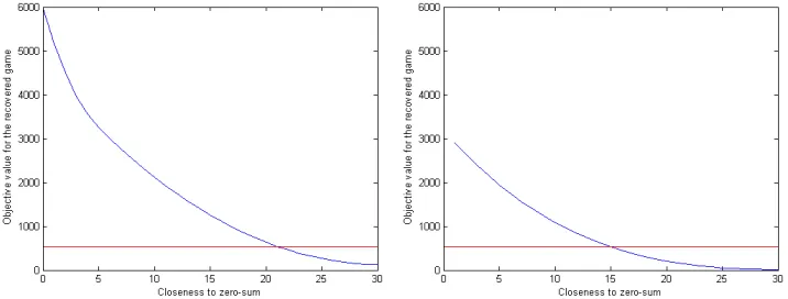
Figure 7.3: Testing for zero-sum with respect to the 1-norm

set of observations is likely to be explained by a zero-sum game. We consider entry games as defined in the previous section, and assume the observer wants to test whether observations were generated by a game that is approximately zero-sum, without any information on the parametric form of the game (the observer does not know the game is an entry game).

Formally, we say a game G = (G1, G2) is ε-zero-sum with respect to the p

-norm if and only if kG1 +G2kp ≤ ε. Note that a game being ε-zero-sum is a linear property and therefore can be included in our framework. The smaller the value of ε, the more stringent the condition is and the closer G is to a zero-sum game. We usel = 500, σ= 0.5,σs = 10 in all simulations.

As before, we pessimistically assume the observer sees δ such that

P(d2(G1, ..., Gl|G)≤δ)≈0.99, i.e. δ= 537.5 for l = 500,σ = 0.5. Figure 7.3

shows for which values of ε one can recover aε-zero-sum game with objective value less than 537.5 that explains the observations for different values of γ

line are impossible, while values to the right of this intersection indicate there is aε-zero-sum game that explain the observations. In both cases, we see that no zero-sum game or game close to being zerosum is a good explanation for the observations; in the payoff information setting, no game less than 21-zerosum explains the observations, while in the payoff shifter setting, no game less than 15-zerosum explains the observations.

7.2 Multiplayer Cournot competition

In this section, we run simulations on a Cournot competition with varying number of players. See Section 6.2 for a discussion of how our framework can be modified to accomodate for Cournot games with many players and an action set of infinite size for each player. All simulations are performed on a laptop with a Intel Core i7-4700MQ at 2.40GHz and 16 Gb RAM.

Generating the games

Letn be the number of players, andqi the production level of playeri. We fix a parameterα= 0.05, and set the price function to be given byP(q1, ..., qn) = 1−α

n

P

i=1

qi; the price function is known to the observer. We fix the form of the cost function to be linear, i.e. the cost of producing qi of goods incurred by player iis given by ci(qi) = aiqi+bi. Without loss of generality, we set bi = 0:

bi does not affect the maximization problem nor the first order condition solved by player iand hence the decision the chosen production level of the players. We generate ng = 10 underlying Cournot games with heterogeneous, linear cost functions ci(x) = aix as follows:

• We first set ˆai = 0.01 for every player i.

• We generate each of the ng games by adding i.i.d. truncated Gaussian noise Xi with mean 0 and standard deviation 0.01 to the ˆai’s. I.e.,

ai = 0.01 +Xi where Xi can be written as Xi =max(Zi,−0.01) andZi is a non-truncated Gaussian with mean 0, standard deviation 0.01. This ensures theai’s are always non-negative, hence the production costs are always non-decreasing.

Note that the same ng games are used in all plots and simulations.