High-resolution multi-band imaging for validation and characterization of small Kepler planets

HIGH-RESOLUTION MULTI-BAND IMAGING FOR VALIDATION

AND CHARACTERIZATION OF SMALL

KEPLER

PLANETS

Mark E. Everett1, Thomas Barclay2,3, David R. Ciardi4, Elliott P. Horch5, Steve B. Howell2,7, Justin R. Crepp6, and David R. Silva1

1

National Optical Astronomy Observatory, 950 North Cherry Avenue Tucson, AZ 85719, USA 2

NASA Ames Research Center, Moffett Field, CA 94035, USA 3

Bay Area Environmental Research Institute, 596 1st Street, West Sonoma, CA 95476, USA 4

NASA Exoplanet Science Institute, 770 South Wilson Avenue, Pasadena, CA 91125, USA 5

Department of Physics, Southern Connecticut State University, 501 Crescent Street, New Haven, CT 06515, USA 6

Department of Physics, University of Notre Dame, 225 Nieuwland Science Hall, Notre Dame, IN 46556, USA

Received 2014 July 15; accepted 2014 November 12; published 2015 January 15

ABSTRACT

High-resolution ground-based optical speckle and near-infrared adaptive optics images are taken to search for stars in close angular proximity to host stars of candidate planets identified by the NASAKeplerMission. Neighboring stars are a potential source of false positive signals. These stars also blend into Kepler light curves, affecting estimated planet properties, and are important for an understanding of planets in multiple star systems. Deep images with high angular resolution help to validate candidate planets by excluding potential background eclipsing binaries as the source of the transit signals. A study of 18 Kepler Object of Interest stars hosting a total of 28 candidate and validated planets is presented. Validation levels are determined for 18 planets against the likelihood of a false positive from a background eclipsing binary. Most of these are validated at the 99% level or higher, includingfive newly validated planets in two systems: Kepler-430 and Kepler-431. The stellar properties of the candidate host stars are determined by supplementing existing literature values with new spectroscopic characterizations. Close neighbors of seven of these stars are examined using multi-wavelength photometry to determine their nature and influence on the candidate planet properties. Most of the close neighbors appear to be gravitationally bound secondaries, while a few are best explained as closely co-alignedfield stars. Revised planet properties are derived for each candidate and validated planet, including cases where the close neighbors are the potential host stars.

Key words:binaries: visual –planetary systems–planets and satellites: detection–planets and satellites: fundamental parameters –surveys– techniques: high angular resolution

1. INTRODUCTION

The NASA Kepler Mission employed a 0.95 m aperture Schmidt telescope in solar orbit for a total of 4 years (2009 May–2013 May).Keplerʼsfocal plane wasfilled with 42 CCDs to collect time series photometry on selected targets in a 115 square degreefield.Keplerdetected transiting exoplanets from a sample of over 150,000 target stars, most of which fell in the Keplermagnitude rangeKp=8–16(Kp, theKeplerbandpass, spans roughly 430–900 nm). The mission was designed to detect and quantify the population of small planets orbiting within or near the habitable zones (HZs) of Sun-like stars

(Borucki et al. 2010). Kepler has produced thousands of candidate planets, dozens of which are good HZ or near-HZ candidates (Batalha et al. 2013). To help confirm the candidates as true exoplanets, the mission has relied on ground-based follow-up observations of the candidate host stars.

The process of producing a list of transiting planets from Keplerdata is a long one. First, raw pixelfluxes are calibrated

(Quintana et al. 2010), and light curves are extracted from apertures and reduced, correcting theflux time series by way of

“cotrending” to remove variations correlated with ancillary spacecraft data(Twicken et al.2010). At the same time, nearby

stars identified in the Kepler Input Catalog (KIC; Brown et al. 2011)are used to estimate blended(excess) flux in the light curves, and this excess flux is removed. Following reduction, the light curves are searched for any significant periodic events similar to those of transiting planets (Jenkins et al.2010). These“threshold crossing events”(TCEs)consist of true planet transits and false positives (events appearing much like planet transits, but attributable to other phenomena). False positives include astrophysical sources like eclipsing binary stars, planets transiting nearby, fainter stars blended with the Kepler Object of Interest (KOI) star, and instrumental artifacts occurring (quasi-)periodically in the time series and which coincide when a light curve is searched on a certain period. Here and after,“KOI star”refers to the brightest star near the center of theKepleraperture as measured in theKepler bandpass (an unambiguous definition for the sample in this study). Cases where the TCEs are due to planets transiting stars other than the KOI are treated as false positives because their planetary properties will have been miscalculated based on adoption of the KOI star properties. Such false positives should be removed from the KOI list, if possible, to maintain it as a well-defined statistical sample. The TCEs are subjected to data validation through a series of automated tests(Wu et al.2010)

and human inspection to weed out obvious false positives. Those TCEs passing data validation are deemed KOIs and given a disposition that identifies some as planet candidates. The term KOI can refer to planet candidates as well as their host stars. The KOI list forms a large and relatively clean

© 2015. The American Astronomical Society. All rights reserved.

7

sample with respect to instrumental false positives, but still contains a significant number of astrophysical false positives. The false positive rate is uncertain, but is likely to be about 10% (Fressin et al. 2013; Santerne et al. 2013). Follow-up observations may be used to identify the false positives and more accurately characterize the host star properties from which planet properties are derived. For example, the high-resolution follow-up imaging described here is used to determine the location and brightness of each star that contributesflux to planet candidate light curves becauseKepler imaging is optimized only for photometry (having 4 wide pixels, typical stellar profiles of~ 6 FWHM and variably sized photometric apertures that are typically several pixels across). The number of confirmed or validated Kepler planets currently stands at 965, which is 23% of the total number of both confirmed and candidate Kepler planets (4233). This relatively small fraction partially reflects the challenges to follow-up observing and analysis needed to confirm planets with a low level of false positive probability.

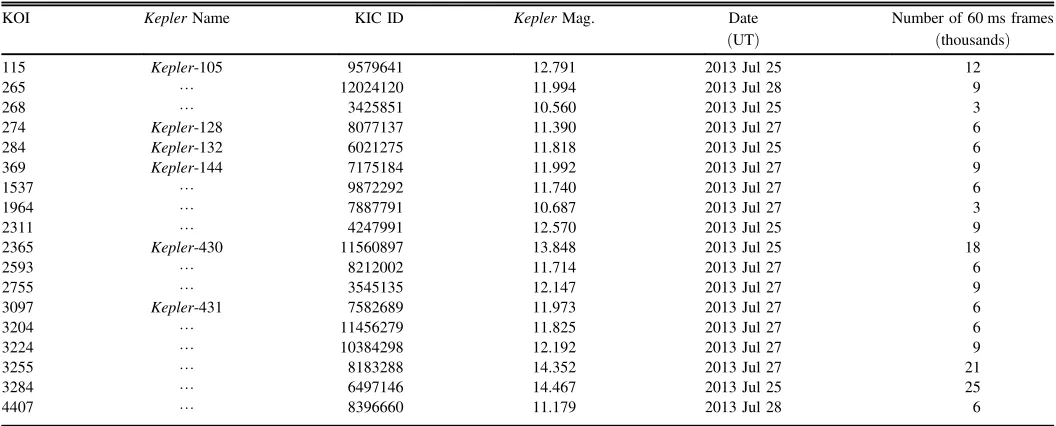
This study presents the analysis of high spatial resolution observations of 18 KOI stars and the 28 validated and candidate planets they harbor. The stellar sample is listed in Table 1. Each KOI star has been observed using high-resolution optical speckle imaging techniques to search for or put limits on the brightness of previously unresolved neighboring stars. Many have also been observed in the near-infrared(near-IR)with adaptive optics(AO)imaging with the same goals in mind. Most of the host stars have been observed spectroscopically to define their stellar properties, while the others have stellar properties available in the literature. The high-resolution imaging is used to calculate a validation level for 18 planets around 12 of these stars by constraining the non-detection of nearby sources. Two new validated planetary systems containingfive planets are designated Kepler-430 and Kepler-431. The effects of blending by neighboring stars are examined and quantified for planets orbiting the seven affected stars and tests are performed that help to distinguish whether these neighboring stars are gravitationally bound companions or field stars. These high-resolution imaging and single epoch spectral observations prove to be an efficient follow-up method

for planet validations and refinement of the planet and host star sample. Such observations lead to a better understanding of the sample of smallKeplerplanets.

2. CANDIDATE PLANET SAMPLE

The sample analyzed here is a set of KOI host stars observed with optical speckle imaging at Gemini North during 2013 July. These targets were selected from the KOI list at the time on the basis of two main considerations: (1) they were not previously observed with high-resolution optical imaging at an 8 m or larger telescope, and(2)they hosted a candidate planet having an estimated radius less than1.5RÅand/or a predicted

planet equilibrium temperature Teq<320K. At the time of target selection there was a total of 750 stars hosting at least one planet meeting this size constraint and 20 stars hosting at least one planet meeting the temperature constraint( tempera-tures low enough to be considered HZ candidates). Since that time, planets have been validated for 140 of these 750 host stars, primarily as part of a validation study of planets in multiple planet systems (Rowe et al.2014), although most of these are lacking the high-resolution imaging needed to thoroughly investigate their possible stellar multiplicity. A total of 25 of the brightest of these 750 stars was observed

(selected to include some with low equilibrium temperature), but 5 of the stars were subsequently found by the mission to be false positive events(mostly cases where the variable was not the KOI, but another star in the aperture). The results for two stars of the sample are discussed separately in the literature: KOI 571(Kepler-186)by Quintana et al.(2014)and KOI 2626 by D. R. Ciardi (in preparation). The remaining 18 stars discussed here (Table 1) hosted a total of 28 candidates

(although some have been subsequently validated).

Along with new observations, analysis of these candidates began by inspecting ground-based data and Kepler data products available from the web site of theKeplerCommunity Follow-up Observing Program (CFOP).8 This included the J-band survey taken at UKIRT(by Phil Lucas)that covers the entireKeplerfield under relatively good seeing conditions(0. 8

Table 1

Speckle Imaging Observations

KOI KeplerName KIC ID KeplerMag. Date Number of 60 ms frames

(UT) (thousands)

115 Kepler-105 9579641 12.791 2013 Jul 25 12

265 L 12024120 11.994 2013 Jul 28 9

268 L 3425851 10.560 2013 Jul 25 3

274 Kepler-128 8077137 11.390 2013 Jul 27 6

284 Kepler-132 6021275 11.818 2013 Jul 25 6

369 Kepler-144 7175184 11.992 2013 Jul 27 9

1537 L 9872292 11.740 2013 Jul 27 6

1964 L 7887791 10.687 2013 Jul 27 3

2311 L 4247991 12.570 2013 Jul 25 9

2365 Kepler-430 11560897 13.848 2013 Jul 25 18

2593 L 8212002 11.714 2013 Jul 27 6

2755 L 3545135 12.147 2013 Jul 27 9

3097 Kepler-431 7582689 11.973 2013 Jul 27 6

3204 L 11456279 11.825 2013 Jul 27 6

3224 L 10384298 12.192 2013 Jul 27 9

3255 L 8183288 14.352 2013 Jul 27 21

3284 L 6497146 14.467 2013 Jul 25 25

4407 L 8396660 11.179 2013 Jul 28 6

8

–0. 9 FWHM ). The J images were examined to locate stars nearby each KOI. Sources as close as~ 1 (corresponding to 408 AU at the mean distance of the stellar sample) could be readily seen in these images, but more importantly they covered areas outside of the relatively small fields of the follow-up high-resolution images. Another data product used were the Kepler Missionʼs data validation reports that show light curves and statistical tests on such things as the motion of stellar centroids in and out of transit, comparison of the depths of odd versus even numbered transits, offsets of the transit relative to predicted positions for the star, and in-transit versus out-of-transit pixel flux differences. The statistics in the validation reports help determine if any of the candidates are particularly suspect as false positives(Bryson et al.2013). The candidates discussed hereafter are“good”candidates in that the inspection uncovered nothing especially indicative of false positives.

3. OBSERVATIONS AND DATA REDUCTION

3.1. Speckle Imaging at Gemini North

Speckle imaging observations were obtained at Gemini North during the interval UT 2013 July 25–31. The Differential Speckle Survey Instrument (DSSI), a dual-channel speckle imaging system described by Horch et al. (2009), was configured with the 692 nmfilter (40 nm FWHM)on thefirst port and the 880 nmfilter(50 nm FWHM)on the second port. While the mounting of the camera went smoothly, there was a light-leak problem in the 880 nm channel on the night of July 25 UT, so the data from that channel was of significantly lower quality and will not be reported here. The problem was identified and eliminated by the start of July 26 UT. The pixel scale and orientation were measured by observing two well-known binary systems, HU 1176(i.e., HIP 83838 or HR 6377) and STT 535 (i.e., HIP 104858 or HR 8123). The known orbital elements from the Sixth Orbit Catalog9 were used to calculate the position angle and separation at the time of the observation, and then compared with the raw pixel coordinates, thereby deriving the scale. Each camera has a slightly different value. Thefinal values were determined to be0. 01076 pixel−1 for the 692 nm camera and 0. 01142 pixel−1 for the 880 nm camera. The position angle difference between pixel axes and celestial coordinates was determined to be5 . 69.◦

Previous experiences and similar observations were taken during 2012 at Gemini North and are described by Horch et al.

(2012). Images were acquired simultaneously in both cameras. The raw data file for each camera consists of 1000 frames

(which is called an“exposure”); at least three exposures were taken for each of the objects and were examined individually and then co-added to achieve the best possible final result. While the objects were acquired and centered on the two detectors with real-time full-frame readout(512 × 512 pixels), the science exposures consisted of frames that were 256 × 256 pixel subarrays, centered on the target. Each frame was 60 ms in duration, meaning each exposure represented 1 minute of integration time. The choice for the number of exposures taken generally followed the magnitude of the target, as one would expect, with the fainter objects receiving more time, but also modified at the telescope depending on seeing, airmass and other factors. Table 1 gives the number of exposures and the

Keplermagnitudes for the systems under study. The seeing for the run varied between approximately FWHM= 0. 5–0. 8, with substantial changes from exposure to exposure for some objects due to weather systems that were in the area at the time

(including Tropical Storm Flossie, which grazed the Hawaiian Islands on UT July 29 and 30). Overall, the data from July 27 represents the bulk of what we present here. This was a relatively calm night with slightly better seeing than the run as a whole.

The basic methodology for speckle data reduction has been described in previous papers, e.g., Howell et al. (2011) and Horch et al.(2012). The latter deals specifically with Gemini data taken in 2012. It is based on Fourier analysis of correlation functions made from the raw speckle data frames. The autocorrelation is used to estimate the modulus of the objectʼs Fourier transform. A point source observation is required to deconvolve the point-spread function(PSF; which amounts to a division in the Fourier domain). The triple correlation function can be used to generate the phase of the object in the Fourier plane. Combining these two functions, an estimate of the Fourier transform of the object is obtained. This is then low-pass filtered with a Gaussian function and inverse transformed to arrive at the final reconstructed image with a diffraction-limited resolution of FWHM 0. 02. Example reconstructed speckle images centered on the double source KOI 1964 are shown in Figure1.

ForKeplerfollow-up observations, we use the reconstructed images to measure the limiting magnitude difference of each observation as a function of distance from the primary star, that is, it is an estimate of the brightest star that could be missed as a function of separation from the primary. As shown in the previous papers, these curves are generally monotonically increasing as a function of separation, meaning that the limiting magnitude near the central star is lower than farther away from the star. Up to the present, we have published5s confidence limits as a function of separation, using all peaks in the reconstructed image to generate a mean and standard deviation of the mean of the peak values. A detectable companion star then must have a peak value larger than the mean plus 5σ. For Gemini data, the results on fainter targets from our run in 2012 July generally showed two image artifacts that were undesir-able in the final reconstructed image: a faint cross pattern centered on the target, and correlated noise patterns over length scales of ~ 0. 05–0. 10. These effects can combine to give a detectability curve with non-Gaussian distribution of peak heights and/or a non-monotonic nature as a function of separation.

We have studied these two effects in the Fourier plane and developed two strategies to reduce their appearance in reconstructed images. First, the cross pattern on the image plane maps to a cross on the Fourier plane, which can be cleanly seen in a region beyond the diffraction limit and removed by replacing the pixel values in the cross with an average of pixel values on either side. Second, the correlated noise appears to be reduced when the point source used to do the deconvolution step is a better match to the point spread function of the target star. Therefore, we have developed an algorithm to “fine-tune” the shape of our point source observation in the Fourier plane based on estimating the difference in dispersion expected for the point source observation and the science target (which is a function of observation time and sky position), and calibrating out the point source dispersion accordingly. These techniques appear

9

to yield reconstructed images which are free of the cross and whose noise peaks have a more Gaussian distribution.

3.2. Near-IR AO Imaging

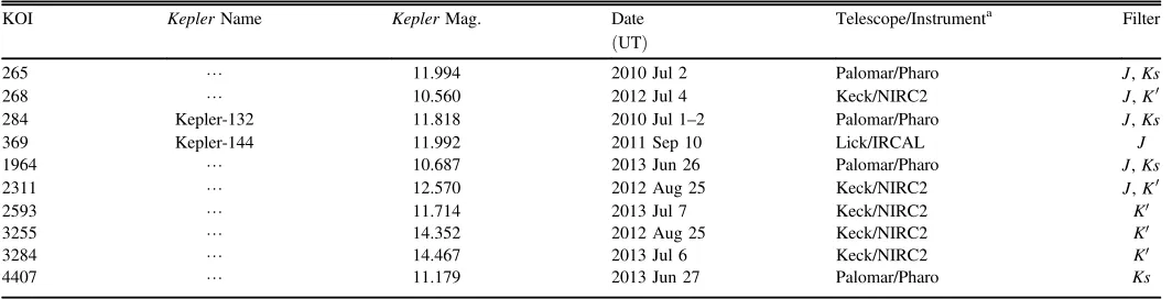
Ten of the KOIs were observed with near-IR AO in theJ,K¢, and Ksfilters either at the Lick Observatory Shane 3.5 m, the Palomar Observatory Hale 5 m, or the 10 m Keck II Telescope

(see Table2), as part of a general infrared AO survey of KOIs

(e.g., Adams et al.2012; Marcy et al.2014; Rowe et al.2014). Targets observed with the Lick, Palomar, or Keck AO systems utilized the IRCAL (Lloyd et al. 2000), PHARO

(Hayward et al. 2001), or NIRC2 (Wizinowich et al. 2004; Johansson et al.2008)instruments, respectively. The observa-tions were made in theJfilter for the Lick observations, theJ Figure 1.Example high-resolution imagery of KOI 1964 and its surroundings in fourfilters. The upper two panels are reconstructed images from speckle observations at 692 nm(upper left)and 880 nm(upper right)taken at Gemini North. The lower two panels are adaptive optics images atJ(lower left)andKs(lower right)taken at the Palomar Hale Telescope. Each image is oriented with North at the top and East to the left. The speckle images are1. 8 ´ 1. 8and the adaptive optics images are approximately15 ´15as seen by the scales. A faint neighbor star is detected0. 4 to the north of the brighter KOI star.

Table 2

Near-infrared Adaptive Optics Observations

KOI KeplerName KeplerMag. Date Telescope/Instrumenta _Filter

(UT)

265 L 11.994 2010 Jul 2 Palomar/Pharo J Ks,

268 L 10.560 2012 Jul 4 Keck/NIRC2 J K, ¢

284 Kepler-132 11.818 2010 Jul 1–2 Palomar/Pharo J Ks,

369 Kepler-144 11.992 2011 Sep 10 Lick/IRCAL J

1964 L 10.687 2013 Jun 26 Palomar/Pharo J Ks,

2311 L 12.570 2012 Aug 25 Keck/NIRC2 J K, ¢

2593 L 11.714 2013 Jul 7 Keck/NIRC2 K′

3255 L 14.352 2012 Aug 25 Keck/NIRC2 K′

3284 L 14.467 2013 Jul 6 Keck/NIRC2 K′

4407 L 11.179 2013 Jun 27 Palomar/Pharo Ks

a

andKsfilters for the Lick and Palomar observations, and theK¢

filter for the Keck observations.

The targets themselves served as natural guide stars and the observations were obtained in a five-point quincunx dither pattern at Lick and Palomar, and a three-point dither pattern at Keck to avoid the lower left quadrant of the NIRC2 array. Five images were collected per dither pattern position, each shifted



1 from the previous dither pattern position to enable the use of the source frames for creating the sky image. The IRCAL array is 256 × 256 with 75 mas pixels and a field of view of

 ´ 

19. 2 19. 2, the PHARO array is 1024 × 1014 with 25 mas pixels and a field of view of 25. 6 ´25. 6, and the NIRC2 array is 1024 × 1024 with 10 mas pixels and afield of view of

 ´  10. 1 10. 1.

Each frame was dark subtracted andflatfielded and the sky frames were constructed for each target from the target frames themselves by median filtering and coadding the 15 or 25 dithered frames. Individual exposure times varied depending on the brightness of the target but typically were 10–30 s frame−1. Data reduction was performed with a custom set of IDL routines.

Aperture photometry was used to obtain the relative magnitudes of stars for those fields with multiple sources. Point source detection limits were estimated in a series of concentric annuli drawn around the star. The separation and widths of the annuli were set to the FWHM of the primary target point spread function. The standard deviation of the background counts is calculated for each annulus, and the5s limits are determined within annular rings (see also Adams et al.2012). The PSF widths for the Lick, Palomar, and Keck images were typically found to be 4 pixels for the three instruments corresponding to 0. 3 , 0. 1 , and 0. 04 FWHM, respectively. Typical contrast levels are 2–3 mag at a separation of 1 FWHM and 7–8 mag at>5FWHM with potentially deeper limits past 10 FHWM. An example of AO imaging done at Palomar toward KOI 1964 is shown in Figure 1.

This study includes observations in both K¢ and Ks filters. The K¢ filter differs only slightly from Ks (with central wavelengths of 2.12 and 2.15 m, respectivelyμ ). Because of this, the differential magnitudes of stars measured in either filter are treated as equivalent since any differences are expected to be slight. For calculations and modeling, the Ks bandpass is used.

3.3. Spectroscopy at National Optical Astronomy Observatory(NOAO)Mayall 4 m

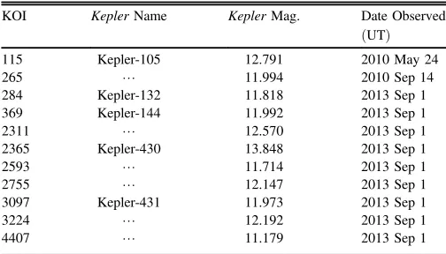
Most of the KOI host stars (16 of 18) were observed spectroscopically at the NOAO Mayall 4 m telescope at Kitt Peak during the 2010 and 2013 observing seasons. Table3lists the 11 spectra actually used to determine stellar properties

(other stars were too cool, too hot, or have published asteroseismology measurements of stellar properties as dis-cussed in Section 4.2). The stars were observed with integration times of 5–15 minutes using the long-slit spectrograph RCSpec setup to disperse the spectra with 0.072 nm pixel−1 at a nominal resolution of δλ = 0.17 nm. The wavelength coverage with the best calibrated fluxes was approximately 380–490 nm. More details of this observing program are discussed in Everett et al.(2013).

Spectral frames are reduced in the manner described by Everett et al. (2013). Briefly, the overscan bias is subtracted and trimmed off each frame. Bias frames and flatfield frames

are then combined, with outlier rejection, to form a master residual bias image andflat. These master frames are applied to each observation in the usual manner. Stellar spectra are extracted using an aperture that traces the stellar image across the CCD and sky-subtracted using night sky spectra extracted from areas of the slit containing sky. Wavelength calibration is provided by an arc lamp exposure at each pointing and flux calibration is done using an observation of a spectrophoto-metric standard star along with a Kitt Peak extinction curve scaled to the airmass of each observation. Since focus changes significantly across the CCD, only the best focused portion of the spectrum is used for analysis(λ=460–489 nm where the focus is tight and important spectral features like Hβ are found).

4. PROPERTIES OF THE KOI STARS

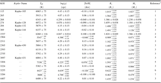
The properties of the candidate host stars are estimated in a number of ways. For most stars, a newly acquired spectrum, taken at the Mayall 4 m telescope, is available as discussed in Section 3.3. In other cases, values are obtained from the literature and are variously based on asteroseismology, photometry, or spectral analysis used in conjunction with light curve fits. Of all stellar properties, the radius is the most fundamental for characterizing transiting exoplanets because it is used to derive the planet radius.

It is worth noting that a number of the candidate host stars have neighboring stars close by. When the apparent separations are small enough, the neighbors can affect both the follow-up photometry and spectroscopy as flux from the neighbor is introduced into the data. However, in most cases the neighbors are at least several magnitudes fainter and so the contamination is slight. To determine the properties of both the KOI star and its neighbors, we take a two-step approach:first, the properties of the KOI star are established from asteroseismology, if available, otherwise spectroscopy or, lastly, photometry when that is the only available source. Second, once the properties of the KOI star are established, the properties of the neighbors are estimated photometrically as will be discussed in Section6.1. In most cases, the photometry of the neighbors is measured relative to the KOI star, so determining the properties of the neighbors depends onfirst characterizing the KOI star.

4.1. New Spectroscopic Properties

In the case of the KOIs observed spectroscopically at the Mayall 4 m telescope, an estimate forTeff,log( )g and[Fe H]is

Table 3 Spectroscopy Observations

KOI KeplerName KeplerMag. Date Observed

(UT)

115 Kepler-105 12.791 2010 May 24

265 L 11.994 2010 Sep 14

284 Kepler-132 11.818 2013 Sep 1

369 Kepler-144 11.992 2013 Sep 1

2311 L 12.570 2013 Sep 1

2365 Kepler-430 13.848 2013 Sep 1

2593 L 11.714 2013 Sep 1

2755 L 12.147 2013 Sep 1

3097 Kepler-431 11.973 2013 Sep 1

3224 L 12.192 2013 Sep 1

made in the manner described in detail by Everett et al.(2013). Very briefly, each spectrum is iteratively fit to a grid of synthetic model spectra taken from Coelho et al.(2005), who parameterized their models using these three properties. The spectral models of Coelho et al.(2005)are based on the stellar atmosphere models of Castelli et al. (2003), and were chosen by Everett et al. (2013) from among the publicly available model spectra for their well-sampled grid in parameter values. The model fitting method is calibrated using a set of similar spectra taken of test stars whose properties were well known a priori. Parameter uncertainties for this method are based on the degree to which the fitted properties of the test star set matched their a priori values. TheTeff,log( )g and[Fe H]values

from these spectra are listed in Table4and marked as coming from reference 1 or 3. A mass, radius and luminosity is determined later for these stars based on isochrone fits (see Section 4.3).

4.2. Properties from the Literature

For some KOIs, we have no 4 m spectrum or the star was such that it could not befit(these spectralfits were reliable only within the effective temperature range 4750 K<Teff<7200 K). For these stars, values ofTeff,log( ), andg [Fe H]are taken from the

literature. The values adopted(in Table4)are those listed in the stellar properties catalog of Huber et al. (2014), which contains

“best available”properties for almost all of the stars targeted by Kepler. It includes properties of very well characterized stars

alongside those based on photometry alone(generally the least reliable method of characterization). For those stars with only photometry, like the hot star KOI 3204, Huber et al.(2014)derive new stellar properties, first by identifying any giants using asteroseismology, thenfindingTefffrom the available photometry.

They determine other parameters with a Bayesian statistical analysis that includes empirically motivated priors on[Fe H]and

g

log( )that help constrain photometric fits of model spectra to optical and near-IR colors. For other stars, Huber et al.(2014)rely on existing data as inputs to the Bayesian analysis. The properties of the cool stars KOI 3255 and KOI 3284 are calculated based on photometrically derived properties from Pinsonneault et al.(2012)

and Dressing & Charbonneau (2013), respectively. For KOI 1964, the constraints are provided by Batalha et al.(2013)and are based on the light curve and spectroscopic fitting techniques described by Buchhave et al. (2012). Three of the KOI stars

(KOIs 268, 274, and 1537)have been analyzed both asteroseis-mologically and spectroscopically by Huber et al. (2013), who provide quite accurate and precise values forTeff,[Fe H],log( ),g



R , andM. For these stars, the mass and radius are the literature values. For all other stars the radii and masses are determined from new isochronefits described next.

4.3. Properties from Isochrone Fits

A new isochrone fitting procedure has been developed for this study to determine the stellar properties for both KOI stars and any potentially bound secondaries (see Section 6.4 for a discussion of neighboring stars’properties). For the purpose of

Table 4 Stellar Properties

KOI KeplerName Teff log(g) [Fe/H] R M Referencea

(K) (cgs) (dex) (R) (M)

115 Kepler-105 6065±75 4.43±0.15 −0.10±0.10 1.015+_-0.189_0.071 1.027+_-0.0350.057 1

265 L 5915±75 4.07±0.15 0.06±0.10 1.564+_-0.456_0.252 1.097+_-0.122_0.054 1

268 L 6343±85 4.259±0.010 −0.040±0.101 1.366±0.026 1.230±0.058 2

274 Kepler-128 6072±75 4.070±0.011 −0.090±0.101 1.659±0.038 1.184±0.074 2

284 Kepler-132 5879±75 4.15±0.15 −0.04±0.10 1.408+_-0.284_0.240 1.023+_-0.080_0.055 3

369 Kepler-144 6157±75 4.14±0.15 −0.02±0.10 +

-1.491 0.288_0.247 1.126+-0.0490.108 3

1537 L 6260±116 4.047±0.014 0.100±0.109 1.824±0.049 1.366±0.101 2

1964 L 5547+_-109₉₁ 4.388+_-0.107_0.126 -0.040_-+0.160_0.140 0.989_-+0.177_0.109 0.871+_-0.068_0.038 4

2311 L 5657±75 4.29±0.15 0.15±0.10 1.182+_-0.220_0.195 0.975+_-0.046_0.039 3

2365 Kepler-430 5884±75 4.15±0.15 0.20±0.10 1.485+_-0.266_0.234 1.166+_-0.0950.134 3

2593 L 6119±75 4.21±0.15 0.16±0.10 1.453+_-0.304_0.287 1.230+_-0.0930.091 3

2755 L 5792±75 4.29±0.15 0.01±0.10 1.172+_-0.236_0.173 0.973+_-0.047_0.037 3

3097 Kepler-431 6004±75 4.40±0.15 0.07±0.10 1.092+_-0.191_0.109 1.071+_-0.0370.059 3

3204 L 7338+_-226₃₃₆ 4.225+_-0.060_0.445 0.070_-+0.170_0.390 1.593+_-1.273_0.202 1.553+_-0.2250.375 5

3224 L 5382±75 4.30±0.15 0.10±0.10 0.962+_-0.100_0.091 0.866+_-0.040_0.021 3

3255 L 4427_-+133₁₂₉ 4.639_-+0.055_0.033 -0.320_-+0.340_0.320 0.622+_-0.056_0.060 0.615+_-0.066_0.049 6

3284 L 3688+_-73₅₀ 4.788+_-0.060_0.080 −0.100±0.100 0.463+_-0.070_0.050 0.479+_-0.060_0.050 7

4407 L 6408±75 4.22±0.15 0.01±0.10 1.435+_-0.329_0.265 1.234+_-0.102_0.065 3

a

1—Teff, log(g)and[Fe/H]from Everett et al.(2013)andRandMfrom this work; 2—all values from the stellar properties catalog(SPC)of Huber et al.(2014) based on data from Huber et al.(2013); 3—stellar properties all from this work; 4—Teff, log(g)and[Fe/H]are SPC values from Huber et al.(2014)based on data from Batalha et al.(2013)andRandMare from this work; 5—all values from the SPC of Huber et al.(2014); 6—Teff, log(g)and[Fe/H]are SPC values from Huber et al.

isochronefitting, each KOI star is described by the set of most probable values for the same three properties (Teff, log( ),g

[Fe H]) with a probability distribution described by half of a normal distribution each for the positive and negative uncertainties (which may differ).

A set of Dartmouth isochrones (Girardi et al. 2005) is constructed using the interpolation software provided with their distribution. The isochrones span an age range between 1–13 Gyr at 0.5 Gyr intervals and metallicity ([Fe H]) range between −0.4 and +0.4 with steps of 0.02 dex with no α-element enhancements. To obtain a finely sampled set of stellar mass points defining each isochrone(where the original isochrones had some large gaps), new points are created using linear interpolation such that the final intervals between successive stellar masses never exceeds 0.02M.

Tofind the properties of the primary star, a probability level is assigned to each mass point in the set of isochrones based on its location in the(Teff,log( ),g [Fe H])probability distribution.

The mass point with the highest probability and the extent of the parameter space mapped out by those points whose probabilities fall inside a certain threshold level define the central values and1suncertainties in the other stellar properties

(e.g.,R and M as listed in Table4and absolute magnitudes as discussed later). Exceptions to this(for Table4)were made for stars with asteroseismology, whose masses and radii are supplied in the available literature.

The precision to which stellar radius is estimated varies between the different techniques. Table 4 lists 12 KOIs with stellar radii derived from spectra without the input of asteroseismology. The mean uncertainty in stellar radius for these stars is 16.9%(averaging all plus and minus uncertainties together). There are three stars with stellar radii based solely on photometric colors with a mean uncertainty of 22.8% (with

uncertainties varying greatly among the sample). The three stars with properties based on asteroseismology have a much lower mean radius uncertainty of 2.3%, illustrating the impact of this technique.

4.4. Magnitudes in the 692 and 880 nm Filters

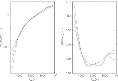
The Dartmouth isochrones already predict absoluteKp,B,V, SDSS griz,J, and Ksmagnitudes, but not magnitudes for the specialized 692 and 880 nmfilters used in speckle imaging. To add absolute magnitudes for the 692 and 880 nmfilters to the isochrone data, color−Teffrelationships are derived that relate

these magnitudes to SDSS magnitudes. These color−Teff

relationships are calculated based on solar metallicity model spectra published by Munari et al. (2005), the filter transmis-sion curves, the QE curve of the DSSI CCDs, an atmospheric extinction curve for Mauna Kea at the typical observing airmass of 1.3, and the AB magnitude system. The color−Teff

relationships between the SDSS magnitudes and speckle imagingfilters are shown in Figure2.

Because the lowestTeffin the model spectra of Munari et al. (2005) was 3500 K, the color−Teffrelationship is linearly

extrapolated down to 2750 K(although the lowestTeffactually

found in the isochrones is ∼3000 K). Additionally, to obtain magnitudes for stars withlog( )g >5, alog( )g =5.5curve is found by linear extrapolation of the colors predicted at

=

g

log( ) 4.5 and 5.0. These extrapolations are indicated in Figure2with light gray lines. For any star defined bylog( )g

andTeff, the absolute magnitudes in the speckle bandpasses can

now be found by interpolating between the two bounding curves in the color−Teffrelationships given their absolutegorz

magnitudes. These calculations are done assuming solar metallicity models for each star. Metallicity has a noticeable, but small effect on colors for stars cooler than 4000 K which

Figure 2.Relationships between stellar effective temperatures and colors relating the 692 nm to the SDSSrfilter(left panel)and the 880 nm to the SDSSzfilter(right panel). These colors are calculated based on model stellar spectra for3500⩽ Teff⩽104K atlog( )g values of 4.0(black dashed line), 4.5(black solid line), and 5.0

increases with decreasing effective temperature. At Teff = 3000 K, there are color differences of ∼0.02 in 880 -z

and∼0.15 in692-rwhen comparing[Fe H]=−0.5 models to solar metallicity models. Thus, there is additional uncertainty in modelingfluxes in the specklefilters among cool stars. This mainly impacts a few of the faint neighbor stars discussed in Section 6.

5. FALSE POSITIVE PROBABILITY ANALYSIS

A false positive probability is determined for planet candidates orbiting each KOI star that is sufficiently isolated from detectable neighbors such that the KOI star is the only detected star near the source of the candidate signal. This analysis compares the probability of the KOI being a planet host to the probability that a nearly co-aligned and fainterfield star is the source of a false positive signal (i.e., an eclipsing binary or transiting planet). The scenario of an unresolved triple KOI in which two components form an eclipsing pair is not considered here because for these it is difficult to calculate some of the complex scenarios for a given system. Scenarios such as these have been considered by Fressin et al. (2013), who found that the incidence of false positives attributable to an eclipsing secondary component in a hierarchical triple stellar system are quite low, especially among candidates of Neptune and smaller planets like in the sample considered here.

We estimate the false positive probability for each planet candidate by integrating the parameter space not excluded by Kepler data or follow-up observations with respect to a Galactic model. This method is based on the approach described in Barclay et al. (2013) and Wang et al. (2013,

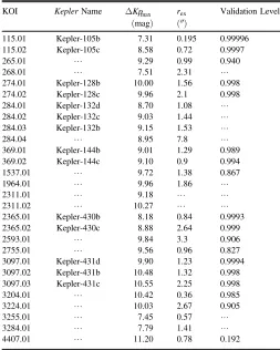
2014). The information used to restrict the parameter space is the transit depth, the Kepler out-of-transit pixel response function (PRF) centroid statistic and the 692 nm Gemini speckle and any near-IR AO observations of the star. The PRF is the observed appearance of point sources and depends on the PSF produced by theKepleroptics, spacecraft jitter, focus, and spectral class of a given point source(although the latter effect is not considered significant enough to treat individually). The measured PRF and its centroid statistic (Bryson et al. 2013), the quarter-by-quarter standard deviation between a stellar centroid in an out-of-transit image and the difference image between in-transit and out-of-transit light curve points are products of theKeplerpipeline(Tenenbaum et al.2013,2014). The transit depth provides a limit on the faintest star that could produce a false positive signal matching the light curve. This comes from assuming a total eclipse by a background eclipsing binary star of identical components, which would produce a 50% eclipse depth. This maximum eclipse depth is adopted under the expectation that for more general binaries with unequal mass components, the larger star will be brighter in the Kepler bandpass. For a maximum eclipse depth, the background star, outside of eclipse, would be DKp_max

magnitudes fainter than the KOI and the observed transit depth can be expressed in terms of δ, the KOIʼs fractional transit depth: DKpmax = -2.5´log (2 )10 d. For example, if the

observed transit depth were 100 ppm, this could be induced by a eclipsing binary of at mostKp=9.25 mag fainter than the KOI. Our estimates of the transit depth are taken from the Keplerdata analysis pipeline(Jenkins et al.2010; Tenenbaum et al.2013,2014). Values forDKp_max are listed in Table5.

TheKeplerout-of-transit PRF centroid statistic is used to set an exclusion radius for each planet candidate. Any star outside

this exclusion radius is excluded from being the source of the candidate transit signal because any such source outside this radius would produce a larger centroid statistic. To find the exclusion radius, we use a 3s threshold where σ is the PRF statistic discussed above. These exclusion radii establish which KOI stars are sufficiently isolated for the analysis as well as restrict the area inside of which false positives are modeled. Values for the exclusion radius,rex, are listed in Table5. In the

case of KOI 2311, no exclusion radius could be determined due to the lack of PRF centroid data on this star. As discussed in Section6, there are eight candidate planets transitingfive KOI stars that show a neighboring star within the exclusion radius. These candidates, plus the two of KOI 2311 are excluded from the validation calculation.

We then include both AO data and DSSI speckle data—we convert the K-band AO data toDKp using the equations of Howell et al.(2012)while we utilize the 692 nm DSSI data and assume no difference between this bandpass and Kp. This provides a brightness-dependent limit on the maximum separation between a target star and a false positive inducing star. The relative brightnesses and angular separations of potential background stars excluded by the photometry, centroid statistics and transit depths for four KOIs are shown in Figure3.

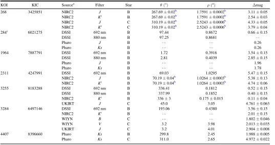
There are 18 candidate planets orbiting 12 stars that qualified for the validation tests. We use the TRILEGAL galactic simulation (Girardi et al. 2012) to first estimate the stellar population within1around the target star. We then integrate the region of parameter space not excluded by observations

Table 5 Planet Validation Results

KOI KeplerName DKp_max rex Validation Level

(mag) (″)

115.01 Kepler-105b 7.31 0.195 0.99996

115.02 Kepler-105c 8.58 0.72 0.9997

265.01 L 9.29 0.99 0.940

268.01 L 7.51 2.31 L

274.01 Kepler-128b 10.00 1.56 0.998

274.02 Kepler-128c 9.96 2.1 0.998

284.01 Kepler-132d 8.70 1.08 L

284.02 Kepler-132c 9.03 1.44 L

284.03 Kepler-132b 9.15 1.53 L

284.04 L 8.95 7.8 L

369.01 Kepler-144b 9.01 1.29 0.989

369.02 Kepler-144c 9.10 0.9 0.994

1537.01 L 9.72 1.38 0.867

1964.01 L 9.96 1.86 L

2311.01 L 9.18 L L

2311.02 L 10.27 L L

2365.01 Kepler-430b 8.18 0.84 0.9993

2365.02 Kepler-430c 8.88 2.64 0.999

2593.01 L 9.84 3.3 0.906

2755.01 L 9.56 0.96 0.827

3097.01 Kepler-431d 9.90 1.23 0.9994

3097.02 Kepler-431b 10.48 1.32 0.998

3097.03 Kepler-431c 10.55 2.25 0.998

3204.01 L 10.42 0.36 0.985

3224.01 L 10.03 2.67 0.905

3255.01 L 7.45 0.57 L

3284.01 L 7.79 1.41 L

with respect to the population model. This provides a number of false positive stars, which is usually much less than 1. We then estimate what fraction of these are likely to be either background eclipsing binaries or background planet hosts

(Slawson et al.2011; Burke et al. 2014). Finally, we compare the number of false positives like this with the predicted number of planets like this across the entire data set. The number of false positives in the entire data set is the number of false positives calculated for this star multiplied by the Kepler sample size of 150,000 (Koch et al. 2010). The predicted number of planets like this is determined by Fressin et al.

(2013). The ratio of the total planets to the total number of planets plus false positives yields the probability that a candidate is a planet.

If the planet candidate is in a multi-planet system we boost the odds that the candidate is a planet by a factor of∼30 for two-candidate systems. This multiplicity boost is justified on the basis of statistics done on theKeplersample(Lissauer et al.

2012,2014). Assuming false positives are randomly distributed among targets, multiple planet systems should not have a higher false positive rate than other targets. It is found that a large fraction of KOIs with at least one planet candidate are found to have at least two candidates, meaning a larger fraction of the planets in these systems are real. Table 5 lists the total validation level for each candidate around an isolated star for which PRF centroid data is available. Two of the systems are designated Kepler-430 and Kepler-431 as newly validated multi-planet host stars hosting a total offive planets validated at

⩾99.8%. The letter designations for these planets are given in the table.

Several of the planets around these KOIs have previous validation calculations done or have been deemed validated. Xie (2014) showed that the two current planet candidates of KOI 274 exhibited anti-correlated transit timing variations, validating both as interacting planets. Wang et al.(2014)used

the native seeing UKIRTJ-band survey images of theKepler field to help calculate validation percentages for the multi-planet KOIs 115, 274, 284, 369, 2311, and 3097, including validation boosting due to their planetary multiplicities. For KOI 115.01 they report a 99.8% validation(considering it part of a three-planet system in contrast to our study that excludes KOI 115.03 due to low detection significance). Wang et al.

(2014) also reported validation levels above 90% for KOIs 115.02 and 284.01, along with lower levels for the other candidates. Rowe et al.(2014)validated a set of multi-planet KOIs including KOIs 115, 274, 284, and 369 by incorporating various tests on theKeplerdata and external data products to arrive at>99% validation levels for their hosted planets.

6. NEIGHBORING STARS

6.1. Observed Properties of Neighboring Stars

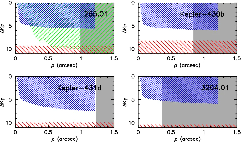
The neighboring point sources (hereafter assumed to be stars)detected around seven of the KOIs in the high-resolution images as well as native seeing survey images are listed in Table 6. The table provides the relative separations (ρ), position angles (θ), and magnitudes fainter than the KOI (D mag). Here, each neighbor star is given a designation of“B”or

“C” as an identifier. These stars could be foreground or background stars that are closely aligned by mere chance with the KOI star or may be gravitationally bound secondaries. The closer and brighter these neighboring stars are, the more likely they are to be gravitationally bound to the KOI, as discussed below.

Table 6 shows that seven KOI stars have a neighbor⩽4 away detected in high-resolution images. In the case offive of these KOIs, one neighbor lies within the exclusion radius for all planet candidates (KOI 268B, 284B, 1964B, 3255B, and 3284B). Such neighbors are potential sources of a false positive(i.e., an eclipsing or transiting system that is blended

Figure 3.Areas of parameter space where data excludes background stars as the source of a false positive planet signal are shown in terms of the relativeKepler

with the KOI). Even very faint neighbors, with magnitudes relative to the KOI star ofΔKp=9–10 can produce a transit-like signal at the level expected for an Earth-sized planet transiting a Sun-like star(Morton & Johnson2011).

The more distant neighbors should not be considered possible sources of a false positive. These stars are nonetheless important to consider as possible members in a stellar binary with the KOI and for their dilution of the KOI light curves. To correct for dilution, a search was made for any star that could possibly dilute the light curve at a 1% level or greater. Both the high-resolution images and other ground-based imaging surveys such as the UKIRT J-band survey and a catalog of UBV photometry by Everett et al. (2012) were used. Some neighbors are left out of this search, namely any listed in the KIC, because any excess flux blended into the light curve by KIC stars will have already been estimated and removed by the Keplerpipeline. Two significant KIC stars were noted near the KOIs in this sample: KIC 11560901, about8. 5 away from KOI 2365(Kepler-430), and KIC 8212005, about12. 9 away from KOI 2593.

6.2. Previous High-resolution Imaging

Several of these stars have been previously observed with high-resolution imaging by Adams et al. (2012, 2013), Law et al. (2014), and Lillo-Box et al. (2014). KOI 1537 was reported by Adams et al.(2013)to have a close neighbor with a separation of 0. 13 in Ks AO images. The same KOI was observed by Law et al. (2014) in an optical AO (RoboAO)

survey of KOIs, but no neighbor was found. Their non-detection would be consistent with the close separation and RoboAO imaging resolution. No neighbor of KOI 1537 is detected in our speckle data. This is surprising given the high spatial resolution, which would easily resolve the separation, and the small magnitude differenceDKs=0.15 reported by Adams et al. (2013). The limiting contrast for detecting neighbors at a separation of0. 13 in the 692 and 880 nm images is 5.37 and 4.69 mag, respectively. These apparently discrepant observations cannot be attributed to a hypothetical very red neighbor. The color880-Ks=1.08is found for KOI 1537 from its isochrone fit, meaning any line-of-sight neighbor would need to be at least as red as880 -Ks5.6, or redder than the reddest stars (880 -Ks=3.9) found in the isochrones of Section 4.3. In light of this observation, KOI 1537 is treated as a single star here. Adams et al. (2012)

observed KOIs 268 and 284 and detected the neighbors of both stars withJandKmagnitude differences in agreement with the values published here. (Note that the position angles they reported for KOI 268 are apparently erroneouslyflipped.)KOI 115 was observed by both Law et al. (2014) and Lillo-Box et al. (2014). It was seen as single by Law et al. (2014), in agreement with our data. Lillo-Box et al.(2014), who observed with a larger field-of-view, reported a neighbor to KOI 115 about4 away and 8 mag fainter in i. Law et al. (2014) and Lillo-Box et al.(2014)also observed KOI 2593. Both reported it as a single source. In addition to KOIs 115, 1537, and 2593, three other stars(KOIs 268, 1964, and 2365)were observed by

Table 6

Neighboring Stars Not listed in theKeplerInput Catalog

KOI KIC Sourcea _{Filter Star θ(°) ρ(″) Δmag}

268 3425851 NIRC2 J B 267.69±0.02b 1.7591±0.0002b 3.11±0.05

NIRC2 K′ B 267.69±0.02b 1.7591±0.0002b 2.54±0.03

NIRC2 J C 310.19±0.02b 2.5243±0.0006b 4.33±0.05

NIRC2 K′ C 310.19±0.02b 2.5243±0.0006b 3.79±0.04

284c 6021275 DSSI 692 nm B 97.44 0.8672 0.66±0.15

DSSI 880 nm B 97.25 0.8681 L

Pharo J B L L 0.26

Pharo Ks B L L 0.26

1964 7887791 DSSI 692 nm B 1.72 0.3916 3.54±0.15

DSSI 880 nm B 2.81 0.4039 2.85±0.15

Pharo J B L L 1.96

Pharo Ks B L L 1.78

2311 4247991 DSSI 692 nm B 69.03 1.0295 5.47±0.15

NIRC2 J B 70.19±0.04b _{1.0264±0.0003}b _5.38±0.13

NIRC2 K′ B 70.19±0.04b _{1.0264±0.0003}b _4.74±0.06

3255 8183288 DSSI 692 nm B 336.41 0.1812 0.52±0.15

DSSI 880 nm B 337.99 0.1852 0.40±0.15

NIRC2 K′ B 336±3 0.175±0.015 0.11±0.04

UKIRT J C 45.0 3.05 4.761±0.063

3284 6497146 DSSI 692 nm B 193.06 0.4380 3.56±0.15

NIRC2 K′ B L L 2.01±0.15

WIYN B C L L 1.802±0.046

WIYN V C 3.2 3.98 2.013±0.035

UKIRT J C 3.2 4.01 2.904±0.008

4407 8396660 Pharo Ks B 299.8 2.45 1.988±0.005

Pharo Ks C 311.0 2.65 4.972±0.022

a

DSSI—Differential Speckle Survey Instrument at Gemini North; Pharo—Near-IR AO imager at Palomar 5 m; NIRC2—near-IR AO imager at Keck II; UKIRT—J-band survey at UKIRT(Phil Lucas, from cfop.ipac.caltech.edu); WIYN—Mosaic2.0 Camera at WIYN 0.9 m(Everett et al.2012).

b

Astrometry based on combination ofJandKsfilters. c

Law et al.(2014)in the optical and, in the case of KOI 1964, in a near-IRKsimage. They reported the closest neighbor to KOI 268 to have an optical magnitude difference of 3.82 ±0.27, which is consistent with our near-IR magnitude differences for a neighbor redder than the KOI. TheirKsobservations of KOI 1964 were in good agreement with ours. They found KOI 2365

(Kepler-430)to be single, again in agreement with our results.

6.3. Distinguishing Bound Companions from Field Stars

Various evidence may be used to determine if neighboring stars are gravitationally bound secondaries or unrelated, line-of-sight field stars. A full simulation of the properties and frequency of secondary stars and field stars could be used. Instead, in this study, a series of simpler tests are applied. These tests consider the brightness of the neighbor, its angular separation from the KOI star, and the stellar colors for those stars observed at multiple wavelengths. Other approaches to using multi-color photometry to investigate the possible physical association of neighbor stars with KOI stars may be found in Gilliland et al.(2014)and Lillo-Box et al.(2014).

6.3.1. Angular Separation and Apparent Brightness

First, the angular separation from the KOI star and magnitude of the neighbors are examined relative to a random distribution offield stars at the location of the KOI. In doing so, an initial assumption is made that KOI stars are not preferentially co-aligned with unrelatedfield stars. A randomly generated set of stars representing a 1 square degree field is produced at the location of the KOI using the TRILEGAL Galaxy model(Girardi et al.2005, version 1.6 web form. The model predicts apparent magnitudes in various passbands including J and Ks. The number of stars in the TRILEGAL model brighter than the neighbor star is found and multiplied by the ratio of the circular area inside the neighborʼs separation

(ρ)to the 1 square degree model field to get a “background” probability, PBG.PBGis the likelihood that a field star of the

same brightness or brighter than the neighbor would lie by chance at the same or a smaller angular separation from the KOI. In most cases theKsbandpass is used for this calculation because it yields the lowest probabilities. Tofind approximate Ksmagnitudes for the neighbors, the differential photometry of the AO images is used along with the Ks magnitude of the associated 2MASS point source (Skrutskie et al. 2006). For neighbor “C” of KOI 3284, the J magnitude of the UKIRT survey was used instead due to unavailable K-band data. The background probabilities along with the apparent Ks magni-tudes derived for each source are listed in Table 7. As an empirical check on this method, the calculation was also run using Kepler magnitudes of sources extracted from 1 square degree of the KIC at the location of each KOI. The probabilities determined from the KIC agreed with those of the TRILEGAL model to within a factor of 2(some were higher, others lower). Note that in many cases PBG is quite low, a promising

indication that the neighboring stars are gravitationally bound companions. The expectation is that gravitationally bound secondaries outnumber co-aligned neighbors in high-resolution images such as these, especially within separations of ~ 1. 2

(Horch et al.2014). For this reason, these close neighbors are likely dominated by bound companions. However, false positive scenarios for small planet candidate KOIs include the case of large planets transiting background (or field)stars

that are closely co-aligned with the KOIs. These cases can appear much like the observed double KOI sources we have detected in terms of relative magnitude and separation(Fressin et al. 2013). For these cases, the assumption that background stars are randomly distributed in the sky is invalid and the low values ofPBGare best treated as just one of several indicators

that help distinguish between field stars and bound compa-nions. These probabilities are most applicable for neighbor stars that lie outside the exclusion radius. On the other hand, a low value ofPBGfor a neighbor star inside the exclusion radius

can be explained as either a bound companion or a false positive.

6.3.2. Colors and Relative Brightness of Neighbors

Both stars of gravitationally bound pairs should lie on the same isochrone and this can be tested for KOIs that have been observed at multiple wavelengths. The test relies on the relative brightnesses and colors of the two stars. To determine these, the isochronefits are used tofind the colors of the KOI stars while the differential photometry of the imaging provides relative colors and brightnesses of the neighbor. Table 8 lists the relative brightnesses and colors for the double KOI sources that have been observed in more than onefilter. The magnitudes in the table are absolute magnitudes for the KOI stars and likewise for their neighbor stars if they are gravitationally bound. Figure4compares the magnitudes and colors of six KOI stars and their close neighbors alongside the isochrones describing the KOI star properties. The colors and magnitudes of each KOI star(within its1suncertainty range)are indicated by dark gray regions in each panel. The light gray regions show the set of isochrones that pass through these ranges of uncertainty. The magnitudes in each plot represent absolute magnitude as predicted by the Dartmouth isochrones or, in the case of the 692 and 880 nmfilters, calculated from the isochrones’SDSS magnitudes as described in Section4.4. The relative magnitude and colors of the neighbors with respect to the KOI stars are calculated using the relative photometry provided by the speckle imaging analysis and near-IR AO images. The neighboring stars’ colors and magnitudes are shown as rectangular boxes that indicate the 1s photometric uncertainties.

6.3.3. Color Relative to Background Population

To compare the colors of the close neighbors of six KOI stars to the colors offield stars of the same apparent brightness, the TRILEGAL Galaxy models are used again (the same 1 square degree field populations used in Section 6.3.1). This time thefield star populations are restricted to those stars within 1 mag of the apparent magnitude of the neighbor star in the bluer of twofilters being considered. The number offield stars is plotted as a function of colors in Figure5. The colors of the neighboring stars are indicated by vertical lines (solid lines represent the central value and dotted lines the1s uncertainty interval).

The color distributions of thefield stars show several features. InJ-Ks, the peak near 0.25 is due to large numbers of upper main sequence plus turn-off stars, a second peak near 0.6 is due to giants, and some plots show a peak at 0.75 due to lower main sequence dwarfs. The same features are seen in692-Ks at 1.1, 1.8, and 2.25, respectively. The upper Main Sequence plus turn-off stars and giants show up as peaks near 0 and 0.15, respectively, in692-880. The red tails of the692 -880and

-Ks

692 colors are comprised of the lowest mass dwarfs. The field star color distributions are affected by reddening while the colors derived for the secondary stars are intrinsic colors (zero reddening effects). However, extinction is quite small in the TRILEGAL models where AV = 0.03–0.04 to Table 7

KOI Neighbors Considered as Bound Companions

KOI Component θ(°) ρ(″) ApparentKpa _P

BG Filter Kpb s

- < >

Kp Kp Kp

b

( )

268 KOI L L 10.56 L L 3.56±0.10 L

268 B 267.69 1.7591 14.88 5.1´10-4 _Ks +

-7.87 0.13_0.11 −0.10

268 B 267.69 1.7591 14.88 L J 7.89+_-0.14_0.10 0.07

268 C 310.19 2.5243 16.59 2.5´10-3 _Ks +

-9.59 0.09_0.07 0.0

268 C 310.19 2.5243 16.59 L J 9.59_-+_0.090.11 0.0

284c KOI L L 12.38 L L 3.75_-+_0.400.41 L

284 B 97.44 0.867 12.80 4.8´10-5 _Ks +

-4.02 0.45_0.46 −0.32

284 B 97.44 0.867 12.80 L J 4.02+_-0.42_0.44 −0.34

284 B 97.44 0.867 12.80 L 692 nm 4.41+_-0.44_0.40 0.61

1964 KOI L L 10.73 L L 4.78_-+0.23_0.26 L

1964 B 2.26 0.3978 14.10 1.2´10-5 _Ks +

-8.00 0.33_0.34 −0.46

1964 B 2.26 0.3978 14.10 L J 7.64+_-0.30_0.36 −1.74

1964 B 2.26 0.3978 14.10 L 880 nm 8.36+_-0.30_0.29 0.70

1964 B 2.26 0.3978 14.10 L 692 nm +

-8.38 0.23_0.22 1.05

2311 KOI L L 12.57 L L 4.29+_-0.39_0.37 L

2311 B 70.19 1.0264 19.02 2.1´10-3 _Ks +

-11.32 0.37_0.46 1.26

2311 B 70.19 1.0264 19.02 L J 11.59+_-0.40_0.44 1.92

2311 B 70.19 1.0264 19.02 L 692 nm +

-9.72 0.38_0.36 −2.70

3255 KOI L L 14.92 L L 7.04+_-0.22_0.23 L

3255 B 337.20 0.1832 15.33 1.3´10-5 _{Ks 7.25±0.21 −0.90}

3255 B 337.20 0.1832 15.33 L 880 nm +

-7.54 0.27_0.22 0.46

3255 B 337.20 0.1832 15.33 L 692 nm 7.54+_-0.26_0.22 0.46

3255 C 45.0 3.05 19.77 6.2´10-2 _J +

-12.73 0.24_0.13 L

3284 KOI L L 14.55 L L 8.89+_-0.17_0.22 L

3284 B 193.06 0.4380 17.32 4.6´10-5 _{Ks 11.28±0.19 −2.07}

3284 B 193.06 0.4380 17.32 L 692 nm 12.29+_-0.19_0.24 2.62

3284 C 3.2 4.01 16.73 9.2´10-3 _J +

-12.35 0.13_0.18 6.53

3284 C 3.2 4.01 16.73 L V 10.71+_-0.19_0.24 −2.33

3284 C 3.2 4.01 16.73 L B 10.45+_-0.17_0.24 −4.02

4407 KOI L L 11.18 L L 3.34+_-0.44_0.45 L

4407 B 299.8 2.45 14.36 1.9´10-3 _Ks +

-6.52 0.89_1.01 L

4407 C 311.0 2.65 18.64 2.5´10-2 _Ks +

-10.80 0.49_0.54 

a

In this columnKpmagnitudes for secondary stars are mean values based on a combination of allfilters(Section6.4.1). b

In these columnsKprefers to absoluteKeplermagnitudes, which are calculated independently for eachfilter. c

distant lines of sight in the Kepler field and so reddening corrections in the 692-Ks color would be only 0.02–0.03 mag using the extinction curve of Cardelli et al.

(1989). For this reason, no adjustment for the effects of reddening has been made.

In each panel of Figure5, the colors of the neighbor stars are either consistent with the bulk of the field star distribution or redder than it. Assumingfield stars are distributed randomly on the sky around each KOI, afirst order expectation is that their colors will be drawn from this same distribution. For this reason, the relatively red colors of the neighbors seen in panels

(e),(f),(i),(k), and(l) (i.e., KOI 1964B, 2311B, 3255B, and 3284B)are best explained by low-mass gravitationally bound secondaries (although the extreme color measured for KOI 3284B was difficult to explain as discussed earlier). Two other neighbor stars, KOI 268B and C (panels (a) and

(b))are also quite red, but so too are morefield stars inJ-Ks.

6.3.4. Assessing the Nature of Each Neighbor Star

None of the observations definitively distinguishes between gravitationally bound orfield star neighbors, but in most cases the evidence points toward the close neighbor being a gravitationally bound secondary. Values of PBG are quite

small for all but the three most distant neighbors(KOI 3255C, KOI 3284C, and KOI 4407C), which means these have a reasonable likelihood of being nearby field stars. KOI 1964B and KOI 2311B also show some evidence of being field stars based on some colors (J-Ksin the case of KOI 1964B and

-Ks

692 in the case of KOI 2311B). However, KOI 1964B is less conclusive because in the other colors examined it appears to be a relatively low-mass, red, bound companion. The photometry for KOI 3284C is inconsistent with that of a binary companion, but is internally consistent with that of a background dwarf(see Section6.4.2).

The other five neighbors with multi-band photometry

(KOIs 268B, 268C, 284B, 3255B, and 3284B) are the most consistent with being bound companions. KOI 3255C has photometry inJonly and KOI 4407B and C inKsonly, so their natures remain indeterminate.

Overall, among the 11 neighbor stars in this study, 8 have multi-band photometry. Of those eight,five are deemed likely bound companions, one a likely field star, and the 2 others remain too ambiguous to classify. Based on this, the fraction of likely bound companions may be as high as 87.5% or as low as 62.5%. This can be compared to the lucky imaging survey of 174 candidate or confirmed KOI host stars by Lillo-Box et al.

(2014). Among their targets observed in both i and z filters, five were found with close companions, but they considered only one of them to be a bound companion. The significance of the lower fraction of bound companions is difficult to quantify, but given the larger mean separations for the companions in the Lillo-Box et al. (2014) survey, a greater fraction of field stars is reasonable. In a study of 23 KOIs observed in 2filters withHubble Space Telescope Wide Field Camera 3, Gilliland et al.(2014)quantified the odds for neighboring stars to be the bound companions of KOIs. They found eight neighboring stars were physically associated with the target KOI, and six of these had relatively close separations of< 1 . Clearly, high-resolution imaging inside of~ 1 is needed tofind most of the wide binary companions to KOIs.

6.4. Blending Corrections for Crowded KOIs

In order to correct the light curves for the effects of blending, neighbors’ stellar properties must be estimated. Two separate scenarios are considered for the status of these neighbor stars: bound companions and unrelatedfield stars. For completeness, and because most of the neighbor stars are consistent with being gravitationally bound secondaries, a calculation is made for each neighbor assuming it is gravitationally bound. In the case of binaries, the secondary star properties are more easily

Table 8

Magnitudes and Colors of KOI Stars and their Neighborsa

KOI Component 692 nm 880 nm J Ks 692 nm−880 nm 692 nm−Ks J-Ks

268 KOI +

-3.58 0.10_0.09 3.63+_-0.10_0.08 2.82_-+0.09_0.07 2.55_-+0.09_0.06 0.05+_-0.010.00 1.03+_-0.02_0.04 0.27±0.01

268 B L L 5.93+_-0.10_0.09 5.09+_-0.09_0.07 L L 0.84±0.06

268 C L L +

-7.15 0.10_0.09 6.34+_-0.10_0.07 L L 0.81+_-0.06_0.07

284b KOI 3.73+_-0.41_0.39 3.73_-+_0.400.41 2.87_-+_0.400.41 2.53+_-0.41_0.40 0.01±0.01 1.20±0.03 0.34±0.01

284 B +

-4.39 0.44_0.42 L 3.13_-+0.41_0.40 2.79_-+0.41_0.40 L 1.60±0.16 0.34±0.04

1964 KOI 4.73_-+0.23_0.26 4.69+_-0.250.23 3.77+_-0.23_0.24 3.37±0.23 0.04±0.01 1.36+_-0.04_0.05 0.41±0.02

1964 B +

-8.27 0.27_0.30 7.54-+0.270.29

+

-5.73 0.23_0.24 5.15±0.23 0.73±0.21 3.12±0.16 0.59±0.04 2311 KOI 4.24+_-0.39_0.37 4.23_-+0.39_0.37 3.33+_-0.39_0.37 2.95+_-0.39_0.37 0.02±0.01 1.29±0.04 0.37±0.02

2311 B +

-9.71 0.41_0.40 L 8.71-+0.410.39

+

-7.69 0.39_0.37 L 2.02±0.17 1.01±0.14

3255 KOI 6.85+_-0.22_0.21 6.61_-+0.17_0.18 5.43+_-0.16_0.17 4.69_-+_0.150.13 0.24+_-0.06_0.04 2.16+_-0.10_0.11 0.75+_-0.040.03

3255 B 7.37±0.26 _7.01-+0.23

0.24 L

+

-4.80 0.14_0.16 0.36±0.22 2.57-+0.180.19 L 3284 KOI 8.79+_-0.18_0.24 7.99_-+0.14_0.18 6.64_-+0.13_0.16 5.83+_-0.13_0.17 0.80+_-0.06_0.07 2.97_-+0.07_0.09 0.82±0.01

3284 B 12.35+_-0.23_0.28 L L 7.84_-+0.14_0.17 L 4.52+_-0.17_0.18 

a

For KOI stars(labeled as component KOI), magnitudes are absolute values from isochronefits. For neighbors(labeled as component B or C), magnitudes represent absolute values only if they lie at the same distance as the KOI star.

b

constrained by the observations because each component shares a common distance, extinction, composition, and age. The second case, that of neighbor stars being unrelated field stars, is considered for a few cases where evidence suggests or allows this scenario. Constraining the properties of field stars can prove more difficult. To find the stellar properties of assumed secondary stars, the relative photometry is used for isochronefits as described in Section6.4.1. Tofind properties

of field star neighbors, the most likely types of stars are identified in Galaxy models as discussed in Section6.4.2. For either case, an aperture correction is found for each star in Section 6.4.3. Finally, a blending correction, is formulated in Section 6.4.4 based on the Kp magnitudes and aperture corrections for each star in the blend. These corrections are used to reevaluate the planet properties for crowded KOIs as described in Section7.

6.4.1. Properties Assuming Neighbors are Secondary Stars

Each image taken in a different filter provides an independent measurement of the relative brightnesses of the secondary and primary stars. The magnitude differences, along with their observational uncertainties, map the probability distribution of the primary star properties along a set of isochrones into a distribution of secondary star properties. Figure6 shows the distribution of primary and secondary star properties in log( )g and Tefffor the double source KOI 1964

observed in four different filters. Curves outline the range of isochrones used in the model fits.

When relative magnitudes are available in multiple filters, the secondary properties derived from each are combined in a weighted average to obtain a final estimate. One of the most important secondary properties is Kp because it helps to determine the excessflux contributed to the light curve by the secondary. Table 7 lists both apparent and absolute Kp magnitude from the isochrone fits for each multiple KOI

(apparent Kpare mean values calculated from multiple filters and the absoluteKpvalues are individual values for eachfilter). Kepler magnitudes are reported in the KIC for each of the blended KOIs considered here. In cases where neighbors lie



⩽1. 5from the KOI, the KIC magnitude is assumed to be the blend of each component whereas more distant neighbors are assumed to not contribute to the cataloged magnitude of the KOI. Table7 also contains the number of standard deviations each individual filterʼs results are from the mean Kp. These numbers indicate how well data from different passbands

match expectations for a bound companion. The photometry of both neighbors to KOI 268 and the neighbors of KOIs 284 and 3255 agree well with expectations for bound secondaries. The photometry for the neighbor of KOI 1964 agrees less well, but is plausibly consistent with a bound companion. The photo-metry for the neighbors of KOI 3284 and KOI 2311 is inconsistent with a bound companion. This result is similar to the previous analysis indicating these neighbors are likely to be field stars. Table9gives the averaged values ofDKp for each KOI and neighbor based on the individual photometric measurements of each system. This table lists separate values for different planets in multi-candidate systems since the blending situation will later be considered separately for each planet.

6.4.2. Properties Assuming Neighbors are Field Stars

As discussed in Section6.3, there are three neighboring stars with multi-color photometry that show colors plausibly inconsistent with those of a gravitationally bound companion

(KOI 1964B by itsJ-Kscolor, 2311B by its692-Kscolor, and 3284C in all colors). To determine what types offield stars match the observed brightness and colors, the TRILEGAL Galaxy models are used once again. This time the area covered by the Galaxy models is increased to 4 square degrees for KOI 1964 and 10 square degrees for KOI 2311 to ensure a rich sample of model stars. The subset of model stars whose apparent magnitudes lie within 1 mag of the neighbor star and whose colors fall within the observed uncertainty intervals

Figure 6.Results of isochronefits for the double source KOI 1964(an assumed binary star).Teff,log( )g, and[Fe H]for the brighter KOI star(primary)arefitted to a set of Dartmouth isochrones. The probable ranges onlog( )g and log(Teff)for the primary are shown in the shaded region in the upper left of each panel, centered near

=

T