Robot Navigation in Dense Crowds: Statistical Models and Experimental Studies of Human Robot Cooperation

(1)

Robot Navigation in Dense Crowds: Statistical Models and

Experimental Studies of Human Robot Cooperation

Thesis by

Pete Trautman

In Partial Fulfillment of the Requirements

for the Degree of

Doctor of Philosophy

California Institute of Technology

Pasadena, California

2013

(2)

c 2013 Pete Trautman

(3)

(4)

Acknowledgements

My deepest gratitude goes to: Richard Murray, Andreas Krause, Joel Burdick, and Jim Beck. Each

of you provided immense perspective on a vexing problem.

I would also like to thank the staff of Chandler dining hall at Caltech—in particular, Peter Daily

and Jaime Reyes. Without your incredible enthusiasm for technology and robots I would not have

been able to complete my experiments. If only all students of human-robot interaction were so lucky

(5)

Abstract

This thesis explores the problem of mobile robot navigation in dense human crowds. We begin by

considering a fundamental impediment to classical motion planning algorithms called the freezing

robot problem: once the environment surpasses a certain level of complexity, the planner decides

that all forward paths are unsafe, and the robot freezes in place (or performs unnecessary

maneu-vers) to avoid collisions. Since a feasible path typically exists, this behavior is suboptimal. Existing

approaches have focused on reducing predictive uncertainty by employing higher fidelity individual

dynamics models or heuristically limiting the individual predictive covariance to prevent

overcau-tious navigation. We demonstrate that both the individual prediction and the individual predictive

uncertainty have little to do with this undesirable navigation behavior. Additionally, we provide

evidence that dynamic agents are able to navigate in dense crowds by engaging in joint collision

avoidance, cooperatively making room to create feasible trajectories. We accordingly develop

inter-acting Gaussian processes, a prediction density that captures cooperative collision avoidance, and a

“multiple goal” extension that models the goal driven nature of human decision making. Navigation

naturally emerges as a statistic of this distribution.

Most importantly, we empirically validate our models in the Chandler dining hall at Caltech

during peak hours, and in the process, carry out the first extensive quantitative study of robot

navigation in dense human crowds (collecting data on 488 runs). The multiple goal interacting

Gaussian processes algorithm performs comparably with human teleoperators in crowd densities

nearing 1 person/m2_{, while a state of the art noncooperative planner exhibits unsafe behavior more}

than 3 times as often as the multiple goal extension, and twice as often as the basic interacting

Gaussian process approach. Furthermore, a reactive planner based on the widely used dynamic

window approach proves insufficient for crowd densities above 0.55 people/m2_{. We also show that}

our noncooperative planner or our reactive planner capture the salient characteristics of nearly any

dynamic navigation algorithm. For inclusive validation purposes, we show that either our

non-interacting planner or our reactive planner captures the salient characteristics of nearly any existing

dynamic navigation algorithm. Based on these experimental results and theoretical observations, we

conclude that a cooperation model is critical for safe and efficient robot navigation in dense human

(6)

Finally, we produce a large database of ground truth pedestrian crowd data. We make this

ground truth database publicly available for further scientific study of crowd prediction models,

(7)

Chapter 1

Introduction

In this chapter, we review the existing literature on robot navigation in human crowds, introduce

the freezing robot problem, and provide a conceptual explanation of why modeling a cooperative

interaction between humans and robots is critical for successful crowd navigation. We finish the

chapter by detailing the contributions and the organization of the thesis.

1.1

Motivation

One of the first major deployments of an autonomous robot in an unscripted human environment

occurred in the late 1990s at the Deutsches Museum in Bonn, Germany (Burgard et al. [19]). This

RHINO experiment was quickly followed by another robotic tour guide experiment; the robot in the

follow-on study, named MINERVA (Thrun et al. [109]), was exhibited at the Smithsonian and at the

National Museum of American History in Washington D.C. Both the RHINO and MINERVA robots

made extensive use of probabilistic methods for localization and mapping (Roy et al. [90], Dellaert

et al. [24], Roy and Thrun [89]). Additionally, these experiments pioneered the nascent field of human

robot interaction in natural spaces—see Schulte et al. [94] and Thrun et al. [110]. Perhaps most

importantly, the RHINO and MINERVA studies inspired a wide variety of research in the broad

area of robotic navigation in the presence of humans, ranging from additional work with robotic

tour guides (Shiomi et al. [98], Siegwart et al. [101], Shiomi et al. [99], Eppstein et al. [31], Foka and

Trahanias [34], Bauer et al. [8] and Hayashi et al. [45]), to work on nursing home robots (Pineau

et al. [81], Montemerlo et al. [76] and Roy et al. [91]), to robots that perform household chores

(Srinivasa et al. [103] and Kruse et al. [62]), to field trials for interacting robots as social partners

(Kanda et al. [54], Saiki et al. [93], Kruse and et al. [61] and Seifer and Matari´c [96]), to decorum

for robot hosts (Sidner and Lee [100] and Kanda et al. [55]), and even to protocols for social robot

design (Glas et al. [41]).

Despite the many successes of the pioneering RHINO and MINERVA experiments, and the

(11)

crowds remain unresolved. In particular, prevailing algorithms for navigation in dynamic

environ-ments emphasize deterministic and decoupled prediction algorithms (such as in LaValle [68], Latombe

[66] and Choset et al. [22]), and are thus inappropriate for applications in highly uncertain

environ-ments or for situations in which the agent and the robot are dependent on one another. Critically,

a large-scale experimental study of robotic navigation in dense human crowds is unavailable.

In this thesis, we focus on these two deficiencies: a dearth of human-robot cooperative navigation

models and the absence of a systematic study of robot navigation in dense human crowds. We thus

develop a cooperative navigation methodology and conduct the first extensive (nruns ≈500) field

trial of robot navigation innatural human crowds.

1.2

Related Work

Independent agent constant velocity Kalman filters are a starting point for modeling the uncertainty

in dynamic environments. Unfortunately, this prediction engine can lead to an uncertainty explosion

that makes safe and efficient navigation impossible (Figure 1.1). Some research has thus focused

oncontrolling this predictive uncertainty. For instance, in Thompson et al. [108], Bennewitz et al.

[11], Helble and Cameron [49] and Large et al. [65], high fidelity independent human motion models

were developed, in the hope that controlling the predictive uncertainty would lead to improved

navigation performance. The work in Du Toit and Burdick [30] and Du Toit [28] improves navigation

performance by directly limiting individual agent predictive uncertainty. Specifically, they formalize

robot motion planning in dynamic, uncertain environments as a stochastic dynamic program (see

Bertsekas [12, 13]); intractability is avoided with receding horizon control techniques (Mayne et al.

[71], Morari and Lee [77] and Carson [20]). Furthermore, the collision checking algorithms developed

in earlier work (see Du Toit and Burdick [29], which has its roots in Blackmore [15], Blackmore et al.

[17] and Blackmore and Williams [16]) keeps the navigation protocol safe. The insight is that since

replanning is used, the predictive covariance can be held constant at measurement noise. Although

robot-agent interaction models are developed for a few cases, the primary contribution from this

line of research comes in the form of independent agent dynamics models. Section 2.4 argues that

only limiting the uncertainty explosion is insufficient for robot navigation in dense crowds.

The work of Aoude et al. [5, 4] and Joseph et al. [52] shares insight with the approach of Du Toit

[28], although more sophisticated individual models are developed: motion patterns are modeled

as a Gaussian process mixture (Rasmussen and Williams [84]) with a Dirichlet Process prior over

mixture weights (Teh [107]). The Dirichlet process prior allows for representation of an unknown

number of motion patterns, while the Gaussian process allows for variability within a particular

motion pattern. Rapidly exploring random trees (RRT, see LaValle and Kuffner [67]) are used to

(12)

the earlier work in Aoude et al. [3]. No work is done on modeling agent interaction.

The field of proxemics (Hall [42, 43]) has much to say about the interaction between a navigating

robot and a human crowd. Specifically, proxemics tries to understand human proximity relationships,

and in so doing, can provide insight about the design of social robots. In Mead et al. [73, 74] and

Takayama and Pantofaru [105] various robots are developed in accordance with proxemic rules, while

in Mead and Matari´c [72] a probabilistic framework for identifying specific proxemic indicators

is developed. Similarly, Castro-Gonzalez et al. [21] studies pedestrian crossing behaviors using

proxemics. However, this work only studies sparse crowd interactions in scripted settings.

In Svenstrup et al. [104] rapidly-exploring random trees are combined with a potential field

(Khatib [56], Koren and Borenstein [60]); the values in this potential field are based on proxemics.

The authors of Pradhan et al. [83] take a similar proxemic potential function based approach.

Although these navigation algorithms model robot interaction, they do not model

human-robotcooperation. Instead, the emphasis is placed on respecting a proper distance between the robot

and the humans (similar to the work of Ziebart et al. [120]). Further, the algorithm is implemented

in simulation only, and the density of humans in the simulated robotic workspace is kept quite low

(approximately 0.1 person/m2).

Rios-Martinez et al. [87] take a “human-centric” approach as well, but instead of using the

proxemic rules of Hall [42], they use the criteria of Lam et al. [64] instead. They incorporate these

rules of personal space into the robot’s behavior by extending the Risk-RRT algorithm developed

in Fulgenzi et al. [40]. The Risk-RRT algorithm extends the traditional RRT algorithm to include

risk, or the probability of collision along any candidate trajectory.

The mobile robot navigation research in Althoff et al. [1] is more agnostic about the specific

cultural considerations of the dynamic agents. A “probabilistic collision cost” is introduced (to

assess the fitness of candidate robot trajectories in human crowds) that is based on the idea of

inevitable collision states, described in Fraichard and Asama [37] and expanded in Bautin et al. [10]

(inevitable collision states are robot configurations that are guaranteed to result in a collision with

another agent). In particular, Fraichard [36] advocates three quantities as essential to the proper

evaluation of motion safety: the dynamics of the robot, the dynamics of the environment, and a

long enough time horizon. Furthermore, in Fraichard [36] it is argued that full knowledge of these

quantities would enable perfect prediction, which in turn would guarantee perfect collision avoidance.

The cost function of Althoff et al. [1] encodes an approximation of these rules. Importantly, collision

avoidance capabilities of neighboring dynamic agents are modeled. However, experiments are carried

out entirely in simulation.

Importantly, work has been done on learning navigation strategies by observing many example

trajectories. In Ziebart et al. [120], a combination of inverse reinforcement learning and the principle

(13)

data. These methods are extended to the case of a robot navigating through an office environment

in Ziebart et al. [119]: pedestrian decision making is first learned from a large trajectory example

database, and then the robot navigates in a way that causes the least disruption to the human’s

anticipated paths. In Henry et al. [50], the authors extend inverse reinforcement learning to work

in dynamic environments. Their planner is trained using simulated trajectories, and the method

recovers a planner which duplicates the behavior of the simulator. In the work of Waugh et al. [118],

agents learn how to act in multi-agent settings using game theory and the principle of maximum

entropy. The work of Kuderer et al. [63] leverages IRL to learn an interaction model from human

trajectory data. Critically, the IRL feature vector is an extension of the cooperation model that was

developed in Trautman and Krause [114]; thus, not only does this work model cooperation, it pioneers

IRL navigation strategies fromreal human interaction data as well. However the experiments are

limited in scope—one scripted human crosses paths with a single robot in a laboratory environment.

We mention briefly that (although not developed in the field of robotic navigation) models

capturing crowd interaction are explored in Pellegrini et al. [79, 80] and Luber et al. [70] for the

purposes of crowd prediction. These papers rely onthe social forces model, developed in Helbing and

Molnar [46] and Helbing et al. [48, 47]. The ideas introduced in Helbing and Molnar [46] underpin

the interaction model of Chapter 3.

We thus suggest that there is a dearth of human-robot cooperative navigation models, and no

extensive study of robot navigation in dense human crowds has taken place. In this thesis, we

[image:13.612.141.508.433.648.2]

address these two deficiencies.

(14)

1.3

The Freezing Robot Problem

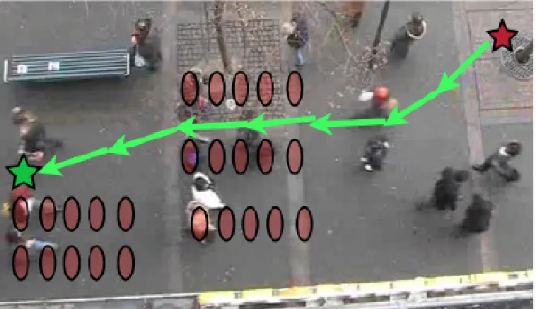
In Figure 1.1, we illustrate thefreezing robot problem. The black star (representing a mobile robot)

predicts the individual trajectories (light red ellipses) of a crowd of people. In this case, the lack of

any predictive covariance constraints results in a robot that cannot make an informed navigation

decision: the deficiencies of the predictive models force the robot to come to a complete stop (or the

robot chooses to follow an essentially arbitrary path through the crowd). As we discuss in Section

5.5.1.1 , arbitrary and highly evasive paths can often be much worse than suboptimal—they can be

dangerous.

Figure 1.1 suggests that the culprit behind the freezing robot problem could be the

individ-ual uncertainty explosion. Indeed, if the amount of uncertainty was the primary reason for this

suboptimal navigation, then using more precise individual dynamics models would prevent the

freezing robot problem. As is illustrated in Figure 1.2, this approach works well for certain crowd

[image:14.612.135.514.323.542.2]

configurations.

Figure 1.2: If the predictive covariance of individual agents is held to a small value, navigation can proceed in an optimal manner—if the crowd is sparse enough.

However, in Section 2.4.1, we show that even underperfect individual prediction(i.e., each agent’s

trajectory isknown to the planning algorithm) the freezing robot problem still occurs if the crowd

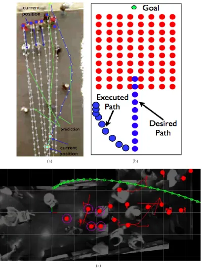
adopts specific configurations. In Figures 1.3(a) and 1.3(b) we illustrate a very common crowd

configuration that can cause any independent planner to fail; when people walk shoulder to shoulder,

the robot is forced to walkaround the crowd, even when the humans are willing to allow passage.

In more demanding scenarios, like the cafeteria illustration in Figure 1.3(c), this behavior can lead

(15)

way for the humans.

As was highlighted in Section 1.2, existing robot navigation approaches commonly ignore

math-ematical models of cooperation between humans and robots. Unfortunately, under this modeling

assumption, the freezing robot problem will always occur, given dense enough crowds.

Given this observation, how is it possible that people can safely navigate through crowds? The

key insight is that people typically engage in joint collision avoidance (this is similar to the social

forces model of Helbing and Molnar [46] and Helbing et al. [48, 47]): they adapt their trajectories

to each other to make room for navigation (see Figure 1.4).

Evidence of the usefulness of joint collision avoidance models occurs in other fields as well: work

on multi-robot coordination in van den Berg et al. [115, 116, 117] and Snape et al. [102] shows that

robots programmed to jointly avoid each other are guaranteed to be collision free and display vastly

improved efficiency at navigation tasks. Additionally, this joint collision avoidance criteria has been

used to improve the data association and target tracking of individuals in human crowds (Pellegrini

et al. [79, 80], Luber et al. [70]).

To our knowledge, however, this principle has not been used to improve robot navigation in

human crowds. Thus, the central idea of this thesis is to explicitly model human-robot interaction

and cooperation in crowds (illustrated in Figure 1.4). To this end, we develop interacting

Gaus-sian processes, a principled statistical model, based on dependent output Gaussian Processes. IGP

(16)

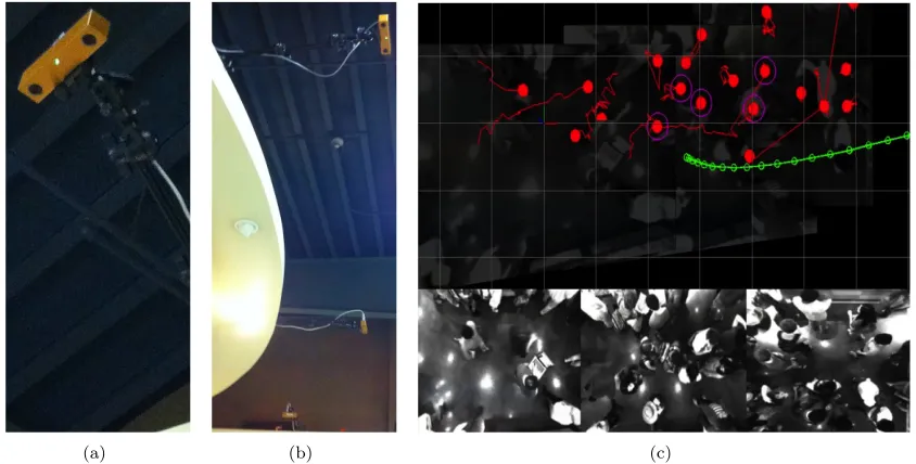
(a) (b)

[image:16.612.123.532.73.618.2]

(c)

Figure 1.3: (a)Even if we hold pedestrian predictive covariance to be extremely small (grey circles), common crowd configurations (shoulder to shoulder walking, sparse crowd) can lead to evasive maneuvering by the robot(b)An illustration of what is occurring in panel(a). Red dots represent crowd prediction, blue dots represent robot decision making(c)Example of freezing robot problem in cafeteria. Robot was not anticipating interaction, and so chose a highly evasive maneuver (green line). Inspection of human tracks (red lines), in contrast, show people passing between each other.

(17)

[image:17.612.120.535.208.541.2]

(18)

1.4

Thesis Contributions and Organization

The remainder of this thesis is organized as follows. Chapter 2 provides further technical background

for the thesis. We define and identify the “freezing robot problem” as a critical impediment to robot

navigation in dense human crowds, and introduce various approaches for solving the freezing robot

problem. Additionally, Chapter 2 introduces Gaussian processes as a novel modeling extension to

existing Markov prediction techniques (such as the Kalman filter).

In Chapter 3, a novel method for modeling cooperation is described, called interacting

Gaus-sian Processes. In particular, this prediction density captures cooperative collision avoidance, the

non-Markov nature of agent trajectories, and the goal driven nature of human decision making.

Additionally, by formulating navigation in dense crowds as a density estimation problem, rather

than a cost optimization problem, we discover an equivalence between inference and planning. This

equivalence provides a novel solution methodology since we can exploit existing approximate

in-ference methods to determine navigation strategies. In particular, we use importance sampling to

approximate the interacting Gaussian processes density. The chapter finishes with a simulation of

how modeling cooperation can improve navigation performance. The results of this simulation serves

as motivation for the quantitative study detailed in Chapter 5.

Chapter 4 provides details about the construction of the robot navigation experiment. We provide

a description of the robotic workspace in Chandler dining hall at Caltech, the pedestrian tracking

system, and the robot itself.

In Chapter 5, we provide the first extensive quantitative study of robot navigation in dense

human crowds (488 runs completed), specifically testing how cooperation models effect navigation

performance. Importantly, we validate the navigation models developed in this thesis, finding, in

particular, that the multiple goal interacting Gaussian processes algorithm performs comparably

with human teleoperators in crowd densities near 1 person/m2_{, while a state of the art}

noncoopera-tive planner exhibits unsafe behavior more than 3 times as often as this multiple goal extension, and

more than twice as often as the basic interacting Gaussian processes. Furthermore, we find that a

re-active planner based on the widely used “dynamic window” approach fails for crowd densities above

0.55 people/m2. We also show that our noncooperative planner or our reactive planner capture the salient characteristics of nearly any dynamic navigation algorithm. Based on these experimental

results and theoretical observations, we conclude that a cooperation model is critical for safe and

efficient robot navigation in dense human crowds.

Finally, Chapter 6 summarizes the contributions of this thesis, provides details on future work

(19)

Chapter 2

Background and Problem Setup

This chapter provides context for the contributions of this thesis. First, since this research is

primarily concerned with robot navigation, we describe some common decision making frameworks.

We introduce robot path planning, decision making under uncertainty and in dynamic environments,

and the principle of receding horizon control. We also describe some approaches to prediction of

dynamic entities. The freezing robot problem, which we discuss in the final section of this chapter,

serves as the motivation for the methods developed in this thesis.

2.1

Discrete Stochastic Optimal Control

We begin by defining some quantities from the field of discrete optimal planning. Letft∈ F ⊆Rnf

be an element of the state space _F. The control (or action) is denoted byuk ∈ U ⊆Rnu_{, where}_U

is the action space. Additionally, letωk (the uncertainty in the system) be distributed according to

some distribution p(ωk). We define the transition function β:F × U × W → F between temporal

states as

ft=β(ft−1, ut−1, wt−1).

Equivalently, we can specify thetransition probability density

p(ft|ft−1, ut−1),

where the uncertainty introduced by ωt−1 produces a probability density function over the next

state. We remark that by applying marginalization, the chain rule of probability (Appendix A.1),

and with knowledge of the initial distribution of the statep(f1), we can recover

p(f2) =

Z

(20)

By iteration, then, we can recover the distribution over any state

p(fT) =

Z

p(fT |fT−1)p(fT−1)dfT−1,

whereT is the end of our prediction horizon. We point out that an implicit dependency assumption

is being made here: each temporal state ft is only dependent on the most recent temporal state

ft−1; this is because the transition function is assumed to befirst order Markov. In Chapter 3 we

generalize the temporal dependency to arbitrary lengths using Gaussian processes for our trajectory

models. Correspondingly, we introduce the boldface notation

f = (f1, f2, . . . fT)

as a shorthand for the entire trajectory. We will use boldface to indicate any quantity over the

duration of an entire trajectory.

Consider furthercontrol policies π:_{F → U} that map states to controls

ut=πt(ft).

Additionally, we define the sequence of control policies overT steps to beπ={π1, π1, . . . , πT}, and

we define a cost function in terms of the control policy:

c(π) =lT+1(fT+1) +

T

X

t=1

lt(ft, πt),

wherelt(ft, πt) is the stage additive cost function. Thus, the expected (Appendix A.3) cost of policy

π is

J(π) =Ef[c(π)].

The optimal policy,π∗=_{π∗₀, π₁∗, . . . , π_T∗₋₁_}, minimizes the expected cost over the set of all admis-sible policies ˜π:

π∗ = arg min

π∈π˜ J(π)

with the optimal cost given by

J(π∗) =E

"

lT+1(fT+1) +

T

X

t=1

lt(ft, πt∗)

#

(21)

Programming. For details on dynamic programming, please consult Bertsekas [12].

For simplicity, we presented here the case of policy search with perfect state information—that

is, we assumed that we could measure the state ft directly through the present time t. This is a

strong assumption, since typical applications involve sensors that produce noisy measurements of

the state, rather than the state itself. Fortunately, if we generalize state space to belief space, the

formulation above (including the use of dynamic programming to find solutions) can still be used.

For details on this transformation consult LaValle [68].

2.2

Receding Horizon Control

The framework of receding horizon control computes policies through online solution of a finite time

optimal planning problem (as in Section 2.1) that can enforce explicit state and control constraints.

In receding horizon control, the computed plan is applied to the system in an open loop manner over

some time interval shorter than the planning horizon. As new information arrives, a new optimal

policy is found and executed. Recursively planning in this manner provides a type of closed-loop

feedback by incorporating current state information into the plan currently being executed.

Mathematically, receding horizon control finds the policy at time t0

π∗t0={πt0, π_t0₊₁, . . . , π_T}

that optimizes

J(πt0) =_E[c(π_t0)]

When implemented in this manner, receding horizon control has proven to be a powerful approximate

planning method (see Carson [20] and Du Toit [28] for example applications).

2.3

Dynamic Agent Prediction

In this section, we present methods for dynamic agent prediction. Kalman filter based prediction

chooses a linear dynamics model for the prediction step (see Appendix A.5), while ignoring the

cor-rection (or update) step, all in a first order Markov framework. Gaussian processes for independent

trajectory models can be viewed as an extension of the Kalman filtering framework.

2.3.1

Kalman Filter Based Prediction

Kalman filters (Kalman [53]) are a special case solution of the sequential Bayesian estimation

equa-tions presented in Appendix A.5. We use xt ∈ Rnx _{to denote the} _state _{variable and} _z

(22)

to denote the measurement variable at time t. Furthermore, for the Kalman filter recursion to be

applicable, the dynamics modelp(xt+1 |xt), the measurement likelihoodp(zt|xt), and the

distri-bution encoding initial knowledgep(x0) all must be Gaussian. These requirements ensure that the

posteriorp(xt|z1:t) is also Gaussian. Rather than specifying these distributions directly, however,

the system and measurement equations can be described:

xt=At−1xt−1+Bt−1ut−1+Ft−1ωt−1

zt=Ctxt+Htνt.

Here, ωt∼ N(0, W) andνt ∼ N(0, V) are independent Gaussian noise terms with covariances W

and V (where _N(µ,Σ) is a Gaussian distribution with mean µ and covariance Σ). The variable

ut−1 is the control input, while the matrixAt−1 is the dynamics model, Bt−1 is the control input

model, Ft−1 is the dynamics noise model, Ct is the measurement model, and Ht is the dynamics

noise model.

This set of linear equations is equivalent to specifying the distributions themselves. For an

interesting take on the system versus distribution point of view, see Ko and Fox [57], where the

authors learn p(xt+1 | xt) and p(zt | xt) (for a remote controlled micro-blimp) using machine

learning techniques, and compare the results to physics based descriptions of the matrices At, Bt

andCt.

2.3.1.1 Prior Kalman Filter

Before the measurement arrives, the Kalman Filter is integrated forward according to the prediction

step of Appendix A.5

p(xt+1|z1:t) =

Z

p(xt+1|xt)p(xt|z1:t)dxt.

Since the dynamics models are linear and Gaussian, we have that

p(xt+1|z1:t) =N(xt+1|xˆt+1:t,Σt+1:t),

whereΣt+1:t∈Rnx×nx. Thus, we need only predict forward the mean and the covariance: ˆ

xt+1:t=Atxˆt:t+Btut

Σt+1:t=AtΣt:tA>t +FtW Ft>.

An example model choice is to encode the zeroeth and first order derivatives inxt, letAtbe a constant

velocity model, ignore inputsut (since the inputs of a dynamic agent are typically unknown), and

(23)

2.3.1.2 Posterior Kalman Filter

Once measurements are collected, the mean and covariance are corrected according to the update

step of Appendix A.5

p(xt+1|z1:t+1) =

p(zt+1|xt+1)p(xt+1|z1:t)

p(zt+1|z1:t)

.

Since the measurement and prediction models are linear and Gaussian, we have that

p(xt+1|z1:t+1) =N(xt+1|xˆt+1:t+1,Σt+1:t+1)

and so we need only correct the mean and the covariance

ˆ

xt+1:t+1= ˆxt+1:t+Kt+1(zt+1−ˆzt+1:t)

Σt+1:t+1= (I−Kt+1Ct+1) Σt+1:t,

where

ˆ

zt+1:t=Ct+1ˆxt+1:t

Kt+1= Σt+1:tCt>+1Γ− 1

t+1:t

Γt+1:t=Ct+1Σt+1:tCt>+1+Ht+1V Ht>+1.

We remark that in the absence of corrective measurements (as is the case for prediction), the

co-variance grows at each incrementing step as

Σt+1:t+1= (I−Kt+1Ct+1)Σt+1:t

=AtΣt:tA>t +FtW Ft>

=Σt+1:t.

Thus, without high fidelity models (i.e., small values forW), prediction can become uninformative

very quickly. We discuss the consequences of this uncertainty explosion in Section 1.3 and in Chapter

2.4.

2.3.2

Gaussian Process Based Prediction

A Gaussian process (see Rasmussen and Williams [84], Ko and Fox [57, 58] and Li et al. [69]) is a

distribution over (typically smooth) functions, and thus well-suited to model wheeled mobile robot

trajectories. Formally, a Gaussian process is a collection of Gaussian random variables indexed by

(24)

function

m: [1, T]→R

(typically taken as zero without loss of generality) and a covariance (or kernel) function

k: [1, T]_×[1, T]_→R.

We will write

f(i)∼GP(m(i), k(i)) to mean that the random function f(i)_{: [1}_{, T}_]

→Ris distributed as a Gaussian process with mean m(i) and covariance k(i); since we will be generalizing to the case of multiple dynamic agents i= 1, . . . n, we introduce the superscript notation i to indicate a particular agent i. For clarification,

we draw a comparison: with a Gaussian vectorx∼ N(µ,Σ), the matrix element Σl,j encodes the

covariance between the elements of the state vectorxl and xj. Likewise, with Gaussian processes,

the kernel function parameterizes the smoothness of the function: recalling that pointst_∈[1, T] act as our index set, we see thatf(i)₍_t_{) and}_f(i)₍_t0_{) are related according to the value of}_k(i)₍_{t, t}0_).

Notionally, we believe the true trajectoryf∗(i) exists (or will exist, since we have only gathered

prior data about this trajectory; see Section 2.3.2.2). The Gaussian processGP(m(i)_{, k}(i)_{) encodes}

all our prior knowledge about the functionf∗(i). In contrast, for sequential Bayesian estimation, the

prior model is typically derived from first principles (such as the physics of the moving object), and

encoded as the distributionp(xt+1 |xt). With Gaussian processes, the prior modelGP(m(i), k(i))

islearned from training data. The dearth of high fidelity first principles models of human behavior,

combined with the abundance of example human trajectory data, make Gaussian processes especially

appealing for our application.

2.3.2.1 Posterior Gaussian Process

For simplicity of notation, we formalize our Gaussian process trajectory model for one-dimensional

locations only. Multiple dimensions are easily incorporated by modeling each dimension as a separate

Gaussian process.

Suppose that we collect the set of noisy measurements z(1:i)t = (z

(i) 1 , . . . ,z

(i)

t ) of the trajectory,

where

(25)

[image:25.612.111.530.55.303.2]

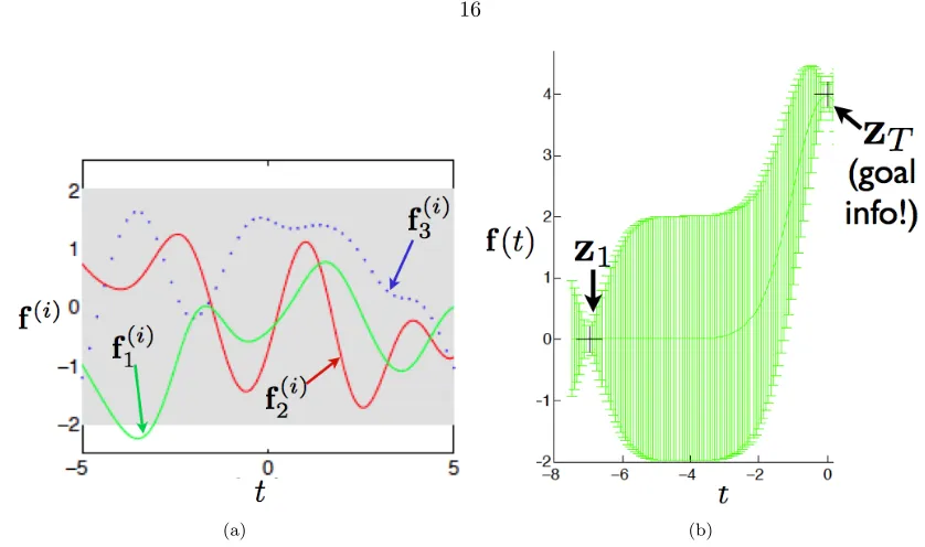
(a) (b)

Figure 2.1: (a)Possible trajectory samples _{fk(i)}k3=1 ∼p(f(i) |z (i)

1:t) from a particular agent i (b)

Using goal informationzT to constrain trajectory prediction.

Then we can calculate the posterior Gaussian processp(f(i)

|z(_1:i)t) =GP(m

(i)

t , k

(i)

t ), where

m(_ti)(t0) = ΣT1:t,t0(Σ1:t,1:t+σ2noiseI)−1z

(i) 1:t

k(_ti)(t1, t2) =k(i)(t1, t2)−ΣT1:t,t1(Σ1:t,1:t+σ

2

noiseI)−

1_Σ 1:t,t2.

Hereby, Σ1:t,t0 = [k(i)(1, t0), k(i)(2, t0), . . . , k(i)(t, t0)], and Σ_1:_t,_1:_t is the matrix such that the (l, j)

entry is Σl,j = k(i)(l, j) and the indices (l, j) take values from 1 : t. The quantity σ2noise is the

measurement noise (which is assumed to be Gaussian, and as shown in Section 2.3.2.3, can be learned

from training data). Since the entire trajectoryf(i)_{: [1}_{, T}_]

→Ris being modeled, information about the goal of the agent (such as an eating station in a cafeteria) can be treated as a measurementz(Ti).

As illustrated in Figure 2.1(b), the informationz(Ti) constrains the predictive uncertainty along the

entirety of the trajectoryf(i)_{(not only at time}_T_).

2.3.2.2 Training the Gaussian Process

The kernel functionk(i)_{is the crucial ingredient in a Gaussian process model, since it encodes “how”}

the underlying function behaves: in our case, how a dynamic agent moves (e.g., how smoothly, how

linearly, length scales of behavior modes, etc). For a kernel function to be valid it must first be

positive semidefinite. That is, for all sets A that take values in the indexing set (for our case, the

indexing set is the closed continuum [1, T]), ΣA,Amust be positive definite. A class of useful kernel

(26)

kernels can be combined to make new kernels via summation and multiplication.

However, even with this set of predefined kernel functions and rules for combining them, choices

still have to be made. What combination of discrete kernel functions should be used for a particular

application? And once we decide on the kernel functions, how should the kernel hyperparameters

be chosen?

To answer these questions, we begin by assuming that we are presented with a training set of

input-output pairs. For our pedestrian dynamics models, the inputs are the times t0 = 1,2, . . . , t

and the outputs are the trajectory measurementsz(1:i)t. Using this training data we can optimize over

both specific kernel functions as well as the hyperparameters of those particular kernel functions.

Additionally, we describe howa priori information can be leveraged to inform our choice of kernel

function.

Gaussian Process Marginal Likelihood In order to optimize our kernel according to the train-ing data set, we first calculate the probability of the data given the hyperparameters θ and input times_{1, . . . , t_}:

p(z(_1:i)t| {1, . . . , t},θ) =

Z

p(z(_1:i)t|f( i)_,

{1, . . . , t_},θ)p(f(i)

| {1, . . . , t_},θ)df(i)

(this quantity is called the marginal likelihood). Since we have thatf(i)_{| {}₁_{, . . . , t}_{} ∼ N}₍₀_,_Σ 1:t,1:t)

andz(1:i)t|f(

i)_{∼ N} _f(i)_{, σ}2

noiseI

, we can use Appendix A.4.2 to compute the log marginal likelihood:

logp(z1:(it)| {1, . . . , t},θ) =−

1 2(z

(i)

1:t)>(Σ1:t,1:t+σnoise2 I)−

1_z(i) 1:t−

1

2log|Σ1:t,1:t+σ

2

noiseI| −

t

2log 2π.

Each term has an interpretation: the data fit term is ₋1 2(z

(i)

1:t)>(Σ1:t,1:t+σ2noiseI)−1z

(i) 1:t, while

1

2log|Σ1:t,1:t|is a complexity penalty, and

t

2log 2πis the normalization constant.

We set the hyperparameters by maximizing the log marginal likelihood using the partial

deriva-tives with respect to the hyperparametersθj:

∂ ∂θj

logp(z_1:(it)| {1, . . . , t},θ) =−

1 2(z

(i) 1:t)>Σ˜−

1 1:t,1:t

∂( ˜Σ1:t,1:t)

∂θj

˜ Σ−_1:1t,1:tz

(i) 1:t−

1 2tr Σ˜

−1 1:t,1:t

∂( ˜Σ1:t,1:t)

∂θj

!

where ˜Σ1:t,1:t = Σ1:t,1:t+σnoise2 I. Using these derivatives, we can perform standard optimization

routines in order to maximize the hyperparameters. Importantly, we can compare log marginal

likelihood values fordifferent kernel functionsand for kernel functions with different hyperparameter

(27)

2.3.2.3 Gaussian Process Kernels as Pedestrian Dynamics Models

We describe our particular choice of kernel function in this section (up to the hyperparameters,

which are trained using the methods outlined above). Because of the nature of our application

(humans walking through a cafeteria), and the way that we modeled portions of agent trajectories

(see Section 3.1.2), we had a priori insight about which kernel functions were appropriate. For

instance, we were able to rule out thesquared exponential covariance function

kSE(t, t0) = exp

−(t−t

0₎2

2`2_SE

because the functions it encodes are strongly nonlinear. Instead, we chose to model pedestrian

dynamics as the summation of a linear kernel (the nominal movement mode of humans between

waypoints is linear)

klinear(t, t0) =t·t0+

1

γ_linear2 ,

a Matern kernel (it captures mild curving in the trajectory, common to pedestrian dynamics)

kM atern(t, t0) =sM atern· 1 +

√

5(t₋t0)

`M atern

+5(t−t0)

2

3`2

M atern

!

exp ₋ √

5(t₋t0)

`M atern

!

,

and a noise kernel (to account for sensor measurement noise)

knoise(t, t0) =σnoise2 δ(t, t0),

whereδ(t, t0) = 1 ift=t0 and is zero otherwise. Thus, our final kernel was

k(i)(t, t0) =sM atern· 1 +

√

5(t₋t0)

`M atern

+5(t−t0)

2

3`2

M atern

!

exp ₋ √

5(t₋t0)

`M atern

!

+t_·t0+ 1

γ2

linear

+σ2_noiseδ(t, t0).

(Figure 3.1 presents an actual human trajectory exhibiting each of these behavior modes: we observe

linear and curvy motion, and noise in the measurements). Thus, four hyperparameters had to be

learned: sM atern, `M atern, γlinear and σnoise. We used the methods detailed in Section 2.3.2.2 to

train these parameters from sample trajectories.

We point out that, in the absence ofa priori information about what kernel function should be

used, the methods of Section 2.3.2.2 can be used to compare different candidate kernel functions

(e.g., squared exponential versus linear), since the values of the log marginal likelihoods can be

comparedacross different kernel functions. Additionally, comparing marginal likelihood values can

be used to guard against local minima when optimizing a fixed kernel function: for instance, one

might randomly restart the hyperparameter optimization multiple times, and compare the marginal

(28)

hyperparameter set.

2.4

The Freezing Robot Problem

In Section 1.3, thefreezing robot problemwas presented as motivation for the methods developed in

this thesis. In this section we provide mathematical details of the freezing robot problem. We also

provide navigation methodologies for solution of the freezing robot problem that would be useful for

environments like those shown in Figure 2.2.

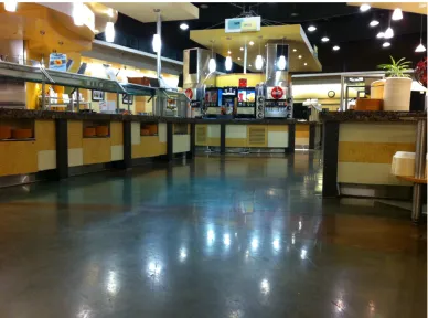
Figure 2.2: Crowded cafeteria at the California Institute of Technology. Because of the many “goal locations” (the pizza bar, the soda fountain, the buffet, etc), distinct traffic currents only rarely materialize. Instead, movement patterns are highly turbulent, as people cross from left to right and top to bottom in a frenzied attempt to grab lunch before their next class. The density and complexity of the crowd ebbs as time moves away from 12pm, allowing for a vast diversity of experiments.

2.4.1

Mathematical Details of the Freezing Robot Problem

Consider agenti, where the indexican take values in the set_{R,1,2, . . . , n_}, such that_{1,2, . . . , n_}

are human agents and i=R is a robot. Suppose we have a distribution p f(i)

over each agent’s

trajectory

(29)

overT timesteps, where each f(i)₍_t_{) = (}_x

t, yt)∈R2 is the planar location of agent iat timet. We also have a likelihood functionp(z(ti)|f(i)(t)) for our observations. Importantly, since we are dealing

with the case of multiple agents, we let

z1:t= (z

(1) 1:t,z

(2) 1:t. . . ,z

(n) 1:t),

acknowledging that for some timest0, we may not observe agenti, in which casez(ti0)=∅. We also

remark that this notation is consistent with Section 2.3.1, since for linear-Gaussian random variables

estimated by a Kalman filter, one can merely augment the state vector with the additional agents.

Figure 2.3 illustrates these quantities.

Figure 2.3: Illustration of the problem and the quantities we are interested in.

In the following, we will assume that data association is solved. Note that an observation of

agenti is not necessarily independent of the robot’s actions. For instance, if the robot’s movement

influences another agent’s movement, then that observationexplicitly depends on the robot’s actions.

Our goal in dynamic navigation is to pick a policy π (see Section 2.1) that adaptively chooses a path f(R) _{for the robot based on the observations} _z

1:t and any ancillary information (such as

agent goal location, boundary locations, etc). The policyπis typically specified by stating thenext

locationf(R)₍_t_{+ 1) the robot should choose given all observational and ancillary information.}

Thus, for any complete sequence of observationsz1:T, the robot can potentially end up choosing

a different pathf(R)₌_π₍_z

1:T). The costJ(π) of a policyπ is the expected cost

J(π) =

Z

p(f,z1:T)c(π(z1:T),f(1), . . . ,f(n))dfdz1:T,

where, for a fixed robot trajectory f(R)_{, the cost function} _c₍_f(R)_,_f(1)_{, . . . ,}_f(n)_{) models the length}

of the path plus penalties for colliding with any of the agents. We use the shorthand notation

f = (f(1)_{, . . . ,}_f(n)_).

(30)

deci-sion process (MDP), where the dimensionality grows linearly with the number of agents, which is

intractable. Intuitively, the intractability is a consequence of attempting exhaustive enumeration;

in the above expected cost J(π), we are attempting to search over the policy space for all possible measurement sequences.

This insolubility is fairly common. In the path planning community, a state of the art, tractable

approximation to this MDP is a method called receding horizon control (RHC), introduced and

explained in Section 2.2. RHCproceeds in a manner similar to MDPs, albeit online: as observations

become available, RHC calculates, based on some cost function, the optimal non-adaptive action

(i.e., fixed path) to take at that time. Indeed, if we letJ(f(R)_|_z

1:t) be the objective function that

calculates the “cost” of each pathf(R)_{based on the observations} _z

1:t, that is

J(f(R)

|z1:t) =

Z

c(f(R)_,_f(1)_{, . . . ,}_f(n)₎_p₍_f

|z1:t)df,

wheref(R)_{is the trajectory of the robot, then}_RHC_finds_f(R_∗)

t , where

ft(R∗)= arg min

f(R)

J(f(R)|z1:t).

As each new observation zτ arrives, for τ > t, a new pathf

(R∗)

τ is calculated and executed until

another observation arrives.

Unfortunately, certain assumptions about the distribution p(f _| z1:t) can cause the minimum

value of the objective function J(f(R∗)

|z1:t) to increase without bound as the number of agentsn

increases. This behavior of the objective function is what we call the freezing robot problem (see

Figure 2.4(d) for an illustration).

To prove this, consider the special case of the objective function where we haveperfect knowledge

of how each pedestrian navigates through the space—that is, we have access to the true state

trajectory ¯z1:T:

p(¯z1:T |f1:T) =δ(¯z1:T −f1:T), (2.1)

wheref_1:(i_T) = [f(i)₍₁₎_,_f(i)₍₂₎_{, . . . ,}_f(i)₍_T_{)], and}_δ₍_a

(31)

this special case, we can compute the objective function:

J(f_1:(RT), n|¯z1:T) =

Z

c(f_1:(RT),f

(1) 1:T, . . . ,f

(n)

1:T)p(f1:T |¯z1:T)df

∝

Z

c(f_1:(RT),f

(1) 1:T, . . . ,f

(n)

1:T)p(¯z1:T |f1:T)p(f1:T)df

=

Z

c(f_1:(RT),f

(1) 1:T, . . . ,f

(n)

1:T)δ(¯z1:T −f1:T)p(f1:T)df

=c(f_1:(RT),¯z

(1) 1:T, . . . ,¯z

(n) 1:T).

We thus see that asnincreases, the minimum value ofJ(f_1:(RT), n|¯z1:T) must also increase—the area

remains fixed, while more of the free space becomes occupied (essentially, the planner must find a

free path through existing open space, with the agent trajectories already traced out).

As the number of agent trajectories increases and thus fills out the fixed navigation area, the

minimum value ofJ(f1:(RT), n|z¯1:T) increases without bound. If we reintroduce missing measurements

and measurement uncertainty, the minimum value of J(f1:(RT), n | z1:T) can only be larger than

J(f1:(RT), n| ¯z1:T) for increasing values of n, since adding uncertainty places nonzero probability of

agent occupation over a larger portion of the space. Thus, J(f_1:(R_T), n_| z1:T) also increases without

bound asnincreases.

Additionally, if we consider theRHC case with perfect observations through time t < T, then

thepredictiveobjective functionJ(f_1:(RT), n|¯z1:t) places nonzero probability of agent occupation over

a larger portion of the space for t0 > t (similar to the case above). Furthermore, if we relax the

objective function to the standard RHC case with measurement uncertainty J(f_1:(RT), n | z1:t), we

further spread uncertainty over times t0 _≤t that have already been observed. Therefore, we have that bothJ(f1:(RT), n|¯z1:t) andJ(f

(R)

1:T, n|z1:t) can only be larger thanJ(f

(R)

1:T, n|¯z1:T), and soRHC

also exhibits freezing robot behavior.

2.4.2

Approaches for Solving the Freezing Robot Problem

In order to fix the freezing robot problem, nearly all state of the art approaches (see Section 1.2)

focus onindividual agent prediction. In particular, Du Toit [28] anticipates the observations

(effec-tively assuming that a certain measurement sequence of theentire trajectory sequence has already

taken place at time t < T); the approach is motivated by the assumption that the culprit of the

freezing robot problem is an uncertainty explosion, illustrated in Figure 2.4(c) and discussed in

Sec-tion 1.3. The claim is that if you can control the covariance, then you can keep the minimum value

of J(f(R)_|_z

1:t) low for moderately dense crowds, and thus solve the freezing robot problem (other

approaches, which incorporate more accurate agent modeling, are similar in motivation, since better

dynamic models would reduce predictive covariance as well). However, as shown above, approaches

(32)

freezing robot problem for crowd densities below a certain threshold; importantly, they cannot be

expected to solve the freezing robot problemin general, no matter how favorable the circumstances

(even for the case of perfect knowledge of the future).

(a) −10(b)−8 −6 −4 −2 0 2 4 6 8 10

−5 0 5 10 15

20 Uncertainty Explosion

(c) Goal Desired Path Executed Path (d)

at time 0, agents too close

together for robot to pass

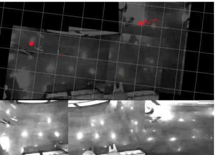
because robot knows about cooperation, FRP avoided Robot proceeds through crowd (e)

Figure 2.4: (a,b)Empirical evidence of joint collision avoidance: blue circles (representing current position) over gray lines are pedestrians moving down, black circles are the area of interest, and green dots are a pedestrian moving upwards. In (a), the blue pedestrians have not yet seen the green person; their projected trajectories (in gray) continue shoulder to shoulder. In (b), green dots surrounded by red circles are the current position of the pedestrian moving up, andall of the pedestrians have adjusted their trajectories to create space—notice how wide the gray prediction has become. It is this joint collision avoidance behavior that we advocate in this thesis. (c-e)Illustration of freezing robot problem. Dynamic crowd agents in red traveling downward, robot we are trying to control in blue. The multiple dots indicate multiple points along one trajectory. (c) Uncertainty explosion due to uncorrected prediction. (d) Even with perfect prediction, room for robot navigation may not exist. (e) Modeling cooperative collision avoidance remedies the freezing robot problem.

This analysis suggests that the planning problem, as described above, is ill-posed. We thus revisit

our probability density,

p(f(1), . . . ,f(n) |z1:t),

and remark that a crucial element is missing—the agent motion model is agnostic of the navigating

robot. One solution is thus immediately apparent: include an interaction between the robots and

the agents (in particular, a joint collision avoidance) in order to lower the cost. We additionally

remark that in the illustration in Figure 2.4(b), the crowd experiments catalogued in the research of

Helbing and Molnar [46], Helbing et al. [48, 47], the multi-robot coordination theorems of van den

Berg et al. [115, 116], and the tracking experiments of Pellegrini et al. [79, 80] and Luber et al. [70], all

corroborate the argument that autonomous dynamic agents utilize joint collision avoidance behaviors

for successful crowd navigation. We thus consider methods to incorporate such an interaction.

(33)

trajectoryf_1:(RT):

p(¯z1:T,¯z( R)

1:T |f1:T,f( R)

1:T) =δ([¯z1:T,¯z( R)

1:T]−[f1:T,f( R) 1:T]).

Notice that because we have coupled the robot’s trajectoryf(R)_{with the agent trajectories}_f _{we can}

now (literally) vary the future joint configurations [¯z1:T,¯z( R)

1:T], and, in turn, vary the minimum value

of the objective function (whereas for Equation 2.1 we were locked into a minimum value that was

based on a fixed value of ¯z1:T). As explained above, approaches that do not consider cooperation

between the robot and the agents fail as soon as the navigation area fills with trajectories (if the

robot is not influencing ¯z1:T, it is unlikely that a free path will emerge randomly); by incorporating

cooperation, however, we are able to manipulate the responses of the agents (i.e., their trajectories)

and thus tocreate space.

We discuss two ways that human-robot interaction (or human-robot cooperation) may be

mod-eled. One approach to modeling this interaction would be to use aconditionaldensityp(f _|z1:t,f(R)),

that encodes assumptions on how the agents react to the robot’s actions, i.e., the idea that all agents

will “give way” to the robot’s trajectory. The problem with this approach is that it assumes that

the robot has the ability to fully control the crowd. Thus, this approach would not only create

an obnoxious robot, but an overaggressive and potentially dangerous one as well. This method is

unsuitable for crowded situations.

The other alternative, which we advocate in this thesis, is to model the robot as one of the

agents, and subsequently model a joint distribution describing their interaction:

p(f(R)_,_f(1)_{, . . . ,}_f(n) |z1:t).

This distribution encodes the idea of cooperative planning (e.g.,cooperative collision avoidance) by

treating robot and agent behaviors as equivalent (unlike the conditional density, where the robot

was given priority, or the noncooperative densityp(f _|z1:t), where the agents were given priority).

We point out an important characteristic of this formulation. Although the robotanticipates agent

cooperation, the data ultimately takes precedence. Consider the situation where an agent does

not cooperate with the robot (perhaps the agent does not see the robot, or perhaps the agent just

does not want to cooperate). As the robot approaches this agent, it will predict that the agent

will eventually act to cooperatively create space. However, as the robot moves closer to the agent,

the evidence (and thus the prediction) that the agent is not going to cooperate will outweigh the

prior belief that agent will cooperate. Thus, the robot will compensate, maneuvering around the

unyielding agent (we observe this behavior in Chapter 5).

With the joint modelp(f(R)_,_f

|z1:t), planning corresponds to computing arg max(f(R)_,_f₎p(f(R),f |

z1:t), i.e., inferring what the robot should do given observations of the other agents (this approach

(34)

Finally, we remark that the formulationp(f(R)_,_f

|z1:t) is independent of the completeness of the

data—that is, z1:t can range from being globally complete (i.e., we are given deterministic access

to each agent’s state at each time t0), to local observations (e.g., an “onboard” sensor that only

observes agents within the line of sight of the robot), to complete data outage. As data reliability

decreases, navigation performance will accordingly degrade, but the method does not require perfect

(35)

Chapter 3

Interacting Gaussian Processes

We begin this chapter by deriving interacting Gaussian processes for crowd prediction. We then

describe how approximate inference is performed on the interacting Gaussian processes density,

followed by a discussion of “the navigation density”, or how robotic navigation in dense human

crowds can be interpreted as a statistic of the interacting Gaussian processes density. We conclude

with the results of a simulation experiment.

3.1

Crowd Prediction Modeling with Interacting Gaussian

Processes

In this section we introduceinteracting Gaussian processes (IGP). Although we ultimately interpret

this density for robot navigation, IGP is also a crowd prediction model. We begin by deriving

individual models of goal driven human motion using mixtures of Gaussian processes. We then

couple these individual models with theinteraction potential.

3.1.1

Gaussian Processes for Modeling Single Goal Trajectories

An advantage to the Gaussian Process formalism (introduced in Section 2.3.2) is that it estimates

entire trajectories. This allows us to incorporate a single goalg(known up to Gaussian uncertainty, g ∼ N(µg, σ2gI)) such that the resulting distribution over trajectories reflects the full impact of

the additional data (Figure 2.1(b) illustrates this idea). Implementation wise, we merely treat the

goal information as a measurement on the final step of the trajectory. That is, having observed

agenti fortsteps, we can augmentz(_1:i)twith z

(i)

T =g. We now update our Gaussian Process using

z(_1:i)_t,T = [z(_1:i)tz

(i)

T ], arriving atp(f

(i)

|z(_1:i)_t,T) =GP(m(_t,Ti), k(_t,Ti)), where

m(_t,Ti)(t0) = ΣT1:t,t0(Σ1:t,1:t+ ˜I)−1z

(i) 1:t,T

k_t,T(i)(t1, t2) =k(t1, t2)−ΣT1:t,t1(Σ1:t,1:t+ ˜I) −1_Σ

(36)

and

˜

I= diag[σ2_noise, σ2_noise, . . . , σ_noise2 , σ2_g].

By varying the amount of noise associated with this goal measurement, we can encode how certain

we are about the goal. Waypoints along trajectories can be easily encoded in the same manner; we

exploit this flexibility in Section 3.1.2.2 to design appropriate models for multi-destination behavior.

For the special case of the robot’s goal, z(_TR), we set the noise differently. The value of σ2

z(_TR)

reflects how precise the robot must be in executing its task. For example, if a robotic arm is to

insert a rivet in an aircraft wing, thenσ2

z(_TR) will be quite small, to reflect aircraft tolerances. If a

robot needs to travel across a busy cafeteria to deliver plates to a human being, then σ2

z(_TR) can be

quite large, perhaps on the order of 1/2 meter or so.

Alternatively, we can derive how goal information should be included using marginalization

followed by the chain rule of probability (see Appendix A.1); this more cumbersome approach will

prove important when we generalize to the case of multiple goals in Section 3.1.2. In particular, we

sum over all possible discrete goal indicesm_∈_N+ _{for the goal variable ¯}_g

m; for eachm, we integrate

over all possible goal arrival times ¯Tm∈R+:

p(f(i)

|z(1:i)t) =

X ¯ gm Z ¯ Tm

p(f(i)_,_(¯_g

m,T¯m)|z

(i) 1:t)

=X ¯ gm Z ¯ Tm p(f(i)

|z(1:i)t,(¯gm,T¯m))p((¯gm,T¯m)|z

(i) 1:t)

=X ¯ gm Z ¯ Tm p(f(i)

|z(1:i)t,(¯gm,T¯m))δ (¯gm,T¯m)−(g, T)

=p(f(i)

|z(_1:i)t,(g, T)).

where δ (¯gm,T¯m)−(g, T)

is 1 when ¯gm = g and ¯Tm = T but zero otherwise. Furthermore,

p((g, T)|z1:t) =δ (¯gm,T¯m)−(g, T)

since we assume knowledge of which goal the agent is going

to (g) and how long it will take to arrive (T). In the final step, we integrate over the variables in the delta function and recover a distribution conditioned on (g, T). Bear in mind that we integrated over the possible goals (see Section 3.1.2.1), not the uncertainty surrounding the location of a

certain goal. Indeed, we still assume that goal location is only known up to Gaussian uncertainty,

g_{∼ N}(µ_g, σ_g2I), and so, if we still wish to model the trajectory prior using Gaussian processes—that is,f(i)

∼GP(0, k(i)_{)—then we recover}

p(f(i)

|z(_1:i)t) =GP(m

(i)

t,T, k

(i)

t,T).

We will use this marginalization-chain rule approach to model situations where we only have

(37)

3.1.2

Gaussian Process Mixtures for Modeling Multiple Goal Trajectories

In practice there may be uncertainty between multiple, discrete goals that an agent could pursue

(Figure 3.1); similarly, it is exceedingly rare to know in advance the time it takes to travel between

these waypoints. For these reasons, we introduce a novel probabilistic model over waypoints and the

transition time between these waypoints. The motion model is then a mixture of Gaussian processes

interpolating between these waypoints.

Figure 3.1: An example trajectory of a cafeteria patron. The trajectory was hand labeled and segmented; blue dots are part of the nominal trajectory (modeled with the kernel function k =

klinear+kmatern+knoise, as in Section 2.3.2.3), green dots are goals (see Section 3.1.2.2), and red

represents interaction between agents (see Section 3.1.3) .

3.1.2.1 Definitions

We begin with the assumption that the environment in which we will be doing trajectory prediction

has a fixed number of goals G (corresponding roughly to the number of eating stations in the

cafeteria):

g= (g1,g2, . . . ,gG)

For the purposes of this analysis, we restrict the distributions governing each goal random variable

(38)

Using data from the cafeteria—the cafeteria floor was first divided into a grid, and then the

amount of time a bin was occupied by a person was collected—we used Gaussian mixture model

clustering (Bishop [14]) to segment the pedestrian track data into “hot spots”. In particular, we

learned

p(g) =

G

X

k=1

βkN gk;µgk,Σgk

.

whereβk is the weight of each component learned,µgk is the mean of the goal location, andΣgk is

the uncertainty around the goal. Figure 3.2 plotsp(g) on top of an image of the cafeteria. Notice that the hotspots occur around the perimeter of the cafeteria, where the food is served.

Figure 3.2: The Gaussian goals identified in the cafeteria. The green dots represent the mean, and the blue and yellow circles represent the length of the covariance axes.

Once we have clustered the data into the distribution p(g), we then need to understand how agents movebetween these goals. For instance, a patron might first go to the pizza station, followed

by the soda fountain, followed by checking out at the cashier bench. We therefore define the transition

probability p(ga → gb) for all a, b ∈ {1,2, . . . , G}. These transition probabilities are empirically

determined from experimental data. For every transition between two goalsga →gb we define the

duration random variable Ta→b, which is governed by a density p(Ta→b) that we also determine

empirically.

Finally, we introduce a waypoint sequence

¯

(39)

(where gmk is a waypoint, andmk ∈ {1,2. . . , G}) for locations indexed bym1, m2, . . . , mF where F _∈_N+, with associated way point durations

¯

Tm={Tm0→m1, Tm1→m2,· · ·, TmF−1→mF}

whereTm0→m1 is the time to the first goal.

3.1.2.2 Generative Process for a Sequence of Waypoints

We now describe a generative process for a sequence of waypoints ¯gm. Beginning with the set

of learned goals g, we draw indices from the set _{1,2, . . . G_}. The first index is drawn uniformly at random1_{, with the following indices drawn according to the transition probability} _p₍_g

a →gb).

Simultaneously, we draw the transition timesTa→b according to the distributionp(Ta→b). We stop

sampling goal points of the sequence ¯gm = (gm1 → gm2 → · · · → gmF) when

PF−1

j=0 Tmj→mj+1

exceeds the prediction horizon T. Notice that the value of F for a particular sequence will not

necessarily match that of another sequence, since the time between goalsTmj→mj+1 varies for allj.

Thus, we can formulate our prediction model for agent i such that we sum over all possible

waypoint sequences ¯gm, and for each particular waypoint sequence ¯gmwe integrate out all possible

associated durations ¯Tm:

p(f(i)|z(1:i)t) =

X ¯ gm Z ¯ Tm

p(f(i),g¯m,T¯m|z

(i) 1:t)

.

Using the chain rule, we end up with

p(f(i)|z(1:i)t) =

X

¯

gm

Z

Tm0→m1 Z

Tm1→m2

· · ·

Z

T_mF₋₁→_mF

p(f(i),g¯m, Tm0→m1, Tm1→m2,· · ·, TmF−1→mF |z (i) 1:t)

! =X ¯ gm Z ¯ Tm

p(f(i)|z(1:i)t,g¯m,T¯m)p(¯gm,T¯m|z

(i)

1:t). (3.1)

Notice that for each goal sequence ¯gm, we potentially have a different number of waypointsgmk.

3.1.3

Interacting Gaussian Processes

Our key modeling idea is to capture the dynamic interactions by introducing dependencies between

the Gaussian processes. We begin with the independent Gaussian process models

p(f(R)

|z(1:Rt)), p(f

(1)

|z(1)1:t), . . . , p(f

(n) |z(1:nt)),

1_{We acknowledge that the parameters}_β

kfrom the mixturep(g) could inform this initial sample. We chose instead

(40)

0

2

4

6

8

10

0

0.2

0.4

0.6

0.8

1

Distance d

ψ

(d)

α

=.8, h=24

α

=.99, h=30

α

=.99, h=24

Figure 3.3: The interaction potential 1₋αexp(₋ 1

2h2d2), for variousα, h.

and couple them by multiplying in aninteraction potential

ψ(f(R)_,_f_{) =}_ψ₍_f(R)_,_f(1)_{, . . . ,}_f(n)₎_,

wheref = (f(1)_{, . . . ,}_f(n)_{). Thus,}

p(f(R)_,_f

|z1:t) =

1

Zψ(f (R)_,_f₎

n

Y

i=R

p(f(i)

|z(1:i)t). (3.2)

The productQn

i=Ris meant to indicate that the robot is included in the calculation. In our

experi-ments, we chose the interaction potential as:

ψ(f(R)_,_f_{) =}

n

Y

i=R n

Y

j=i+1

T

Y

τ=t

1₋αexp ₋ 1 2h2|f

(i)₍_τ₎

−f(j)₍_τ₎ |

where |f(i)₍_τ₎₋_f(j)₍_τ₎_| _{is the Euclidean distance at time} _τ _{between agent} _i _{and agent} _j_{. The}

rationale behind our choice is that any specific instantiation of p

Robot Navigation in Dense Crowds: Statistical Models and Experimental Studies of Human Robot Cooperation