Advance Access publication 2016 March 30
Temporal variability of the wind from the star
τ
Bo¨otis
B. A. Nicholson,
1,2‹A. A. Vidotto,
3,4M. Mengel,
1L. Brookshaw,
1B. Carter,
1P. Petit,
5,6S. C. Marsden,
1S. V. Jeffers,
7R. Fares
8and the BCool Collaboration
1Computational Engineering and Science Research Centre, University of Southern Queensland, Toowoomba, Australia 2European Southern Observatory, Karl Schwarzschild Str. 2, D-85748 Garching, Germany
3Observatoire de l’Universit´e de Gen`eve, Chemin des Maillettes 51, Versoix CH-1290, Switzerland 4School of Physics, Trinity College Dublin, The University of Dublin, Dublin-2, Ireland
5CNRS, Institut de Recherche en Astrophysique et Plan´etologie, 14 Avenue Edouard Belin, F-31400 Toulouse, France 6Universit´e de Toulouse, UPS-OMP, Institut de Recherche en Astrophysique et Plan´etologie, Toulouse, France 7Institut f¨ur Astrophysik, Universit¨at G¨ottingen, Friedrich Hund Platz 1, D-37077 G¨ottingen, Germany 8INAF - Osservatorio Astrofisico di Catania, Via Santa Sofia, 78, I-95123 Catania, Italy
Accepted 2016 March 24. Received 2016 March 24; in original form 2016 January 14
A B S T R A C T
We present new wind models forτ Bo¨otis (τ Boo), a hot-Jupiter-host-star whose observable magnetic cycles makes it a uniquely useful target for our goal of monitoring the temporal vari-ability of stellar winds and their exoplanetary impacts. Using spectropolarimetric observations from May 2009 to January 2015, the most extensive information of this type yet available, to reconstruct the stellar magnetic field, we produce multiple 3D magnetohydrodynamic stellar wind models. Our results show that characteristic changes in the large-scale magnetic field as the star undergoes magnetic cycles produce changes in the wind properties, both globally and locally at the position of the orbiting planet. Whilst the mass loss rate of the star varies by only a minimal amount (∼4 per cent), the rates of angular momentum loss and associated spin-down time-scales are seen to vary widely (up to∼140 per cent), findings consistent with and extending previous research. In addition, we find that temporal variation in the global wind is governed mainly by changes in total magnetic flux rather than changes in wind plasma properties. The magnetic pressure varies with time and location and dominates the stellar wind pressure at the planetary orbit. By assuming a Jovian planetary magnetic field forτ Boo b, we nevertheless conclude that the planetary magnetosphere can remain stable in size for all observed stellar cycle epochs, despite significant changes in the stellar field and the resulting local space weather environment.
Key words: MHD – methods: numerical – stars: individual:τ Bo¨otis – stars: magnetic field – stars: winds, outflows.
1 I N T R O D U C T I O N
The study of stellar winds gives insight into the evolution of stars and the planets that orbit them. The wind affects the stellar rotation rate through mass loss and magnetic braking (Schatzman1962; Weber & Davis1967; Bouvier2013), and can also impact the atmospheres of orbiting planets (Adams2011; Lammer et al.2012), with potential implications on planet habitability (Horner & Jones2010; Vidotto et al.2013). An example of this impact is seen in our own Solar system with the stripping of Mars’ atmosphere by the young Sun (Lundin, Lammer & Ribas2007). However, studying stellar winds is problematic, as winds of stars like our Sun are too diffuse to observe directly (Wood, Linsky & G¨udel2015). Investigation of these stars therefore requires a combination of observation and
E-mail:[email protected]
magnetohydrodynamic (MHD) simulation in order to estimate the properties of these winds.
The starτBo¨otis (τBoo, spectral type F7V) is an ideal candidate for a study of the temporal variability of stellar winds, and their potential impacts on orbiting planets. It is the only star to date, other than our Sun, observed to have a magnetic field cycle, with multiple field reversals observed (Catala et al.2007; Donati et al.
2008; Fares et al.2009; Fares et al.2013; Mengel et al.2016). These observations reveal that the star has a magnetic cyclic period estimated to be a rapid 740 d (Fares et al.2013). The availability of multiple epochs of magnetic field observations allows us to make observationally informed MHD models ofτ Boo’s wind, such as those detailed by Vidotto et al. (2012) (4 epochs observed between June 2006 and July 2008).
In this paper, we present an additional eight MHD simulations of the winds ofτBoo from magnetic field observations taken between
C
2016 The Authors
at University of Southern Queensland on May 3, 2016
http://mnras.oxfordjournals.org/
1908
B. A. Nicholson et al.
May 2009 and January 2015. Our aim is to examine the changes in the wind behaviour due to the variations in the magnetic field over the observed epochs, which include multiple polarity reversals, and to demonstrate how these changes could impact the planetτBoo b. In Section 2, we detail the wind model and magnetic field input. The results of our simulations are presented in two parts: Section 3 presents the global wind properties over the eight epochs, and in Section 4 we investigate the properties of the wind aroundτBoo b and the potential impact of the wind on the planet. We discuss these results in Section 5 and make conclusions based on our findings in Section 6.
2 S T E L L A R W I N D M O D E L
2.1 TheBATS-R-UScode
The stellar wind model used here is the same as used in Vidotto et al. (2012), but with higher resolution (as in Vidotto et al.2014). For simulating the winds we use theBATS-R-UScode (Powell et al.
1999; T´oth et al.2012); a three-dimensional code that solves the ideal MHD equations
∂ρ
∂t + ∇ ·(ρu)=0, (1)
∂(ρu)
∂t + ∇ ·
ρu⊗u+
P+B
2
8π
I−B⊗B
4π
=ρg, (2)
∂B
∂t + ∇ ·(u⊗B−B)=0, (3)
∂
∂t + ∇ ·
u
+P +B
2
8π
− (u·B)B
4π
=ρg·u, (4)
whereρanduare the plasma mass density and velocity,Pis the gas pressure,Bthe magnetic flux, andgis the gravitational acceleration due to a star of massM∗. The total energy density,, is given by
= ρu
2
2 +
P γ−1+
B2
8π. (5)
The polytropic index,γ, is defined such that
P ∝ργ. (6)
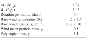
[image:2.595.47.284.294.426.2]Table1lists the stellar and wind values used for this simulation. The values of τ Boo’s mass and radius, M∗ and R∗, are taken from Takeda et al. (2007), and the rotation period,trot, is taken from Fares et al. (2009). The wind mean particle mass,μ, is chosen on the assumption that the wind is only composed of protons and electrons. Each simulation is initialized using a polytropic wind solution and the magnetic field information from observations of a given epoch. It is then iterated forward around 30 000 time steps. This ensures that a steady state is achieved. Each simulation, therefore, is a snapshot of the wind at each epoch.
Table 1. Adopted stellar parameters forτBoo used in the wind model.
M∗(M) 1.34 R∗(R) 1.46 Rotation period,trot(days) 3.0
Base wind temperature (K) 2×10⁶
Base wind density (g cm−3) 8.36×10⁻¹⁶
Wind mean particle mass,μ 0.5
Polytropic index,γ 1.1
2.2 Adopted surface magnetic fields
TheBATS-R-UScode uses a star’s surface magnetic field as input to the inner boundary conditions. The magnetic field information for
τBoo comes from spectropolarimetric observations with the NAR-VAL instrument at T´elescope Bernard Lyot in the Midi Pyr´en´ees, accessed through the BCool collaboration (Marsden et al.2014). The polarization information in the spectra observed at different stellar rotation phases are used to reconstruct the surface magnetic field topologies using Zeeman–Doppler imaging (ZDI, Donati & Landstreet2009). The reconstruction of the magnetic field maps used in this work is presented in Mengel et al. (2016). The radial field topologies are of sole interest for the stellar wind modelling as the other, non-potential field components have been shown to have a negligible effect on the wind solution (Jardine et al.2013).
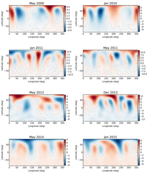
Fig. 1shows the reconstructed radial magnetic fields, in units of Gauss (G), for eight sets of observations (epochs): May 2009, January 2010, January 2011, May 2011, May 2013, December 2013, May 2014 and January 2015. The grey lines here are contours at 0 G. The first three of these epochs were published by Fares et al. (2013); however, for consistency the maps presented here are an updated version using the same methodology as used with the other five epochs, the details of which are presented in Mengel et al. (2016). Due to the inclination of the star, the area below−40◦is not observable. The field in this area of the stellar surface is solved for by enforcing ∇ ·B = 0. Vidotto et al. (2012) showed that choosing this constraint, versus explicitly forcing a symmetric or antisymmetric solution to the large-scale field topology has little impact on the wind solution, especially in the visible hemisphere.
Table2shows a summary of the global magnetic field properties over the observed epochs. The magnetic cycle phase is calculated based on a 740-day cycle found by Fares et al. (2013), with the cycle zero phase chosen to be 2453818 Heliocentric Julian Date (HJD) to align with the magnetic cycle zero-point of Vidotto et al. (2012). The complexity of the field topology can be quantified by examining the amounts of energy in the different set spherical harmonics that are used to describe the field (Donati et al.2006). The modes of these co-efficients wherel≤2 give the dipolar and quadrupolar field config-urations. The complexity of the large-scale field is quantified by the percentage of magnetic energy present in the modes wherel>2 over the total energy. A lower percentage indicates a simpler field con-figuration, whereas a higher percentage means that a larger amount of energy is present in more complicated, smaller scale features.
The field remains dominantly poloidal throughout all observa-tions, with most of the magnetic energy being contained in more complex field components and the complexity varying from 45 per cent to 83 per cent over the cycle. The star is observed to undergo three polarity reversals, with two reversals assumed to have occurred between the May 2011 and May 2013 observations. The absolute surface radial magnetic flux (see Section 3.2) ranges from 1.53× 10²³Maxwells (Mx) to a peak of 3.28×10²³Mx before the polar-ity reversal that was then seen in the May 2014 observations. This same peak and fall in magnetic flux is not observed in the previous polarity reversals probably due to the timing of the observation, and the length of time between observed epochs.
3 W I N D S I M U L AT I O N R E S U LT S : G L O B A L W I N D P R O P E RT I E S
3.1 Magnetic field
The behaviour of the stellar wind is dependent on the geometry and strength of the global stellar magnetic field. Here we examine the
at University of Southern Queensland on May 3, 2016
http://mnras.oxfordjournals.org/
[image:2.595.72.254.663.742.2]Figure 1. Radial magnetic field maps for the eight observed epochs, measured in Gauss (G), with the grey line indicatingBr=0 G. The May 2009 to January
2011 maps come from Fares et al. (2013), and the May 2011 to January 2015 maps from Mengel et al. (2016). The Fares et al. epochs have been reanalysed for consistency with the Mengel et al. maps. The field remains dominantly poloidal across the eight observations, and three polarity reversals are observed. It is believed that two polarity reversals have occurred between May 2011 and May 2013.
behaviour of the wind at intervals of five months to one year, over a total period of five years and seven months. It is expected that the wind will vary little over the time it takes to observe one epoch (∼14 d; Vidotto et al.2012).
As the magnetic field extends outward from the stellar surface, it will be influenced by the presence of the stellar wind. Fig.2shows the magnetic field lines (grey lines) outwards from the surface of the star. The colour contours on the surface represent radial magnetic
at University of Southern Queensland on May 3, 2016
http://mnras.oxfordjournals.org/
1910
B. A. Nicholson et al.
Table 2. Summary of the radial magnetic field polarity and com-plexity ofτBoo for observations from May 2009 to January 2015. The magnetic cycle period is taken to be 740 d from Fares et al. (2013), with the phase zero-point at 2453818 HJD.
Date Magnetic Visible pole Radial field cycle phase polarity complexity
(per cent ofl>2)
May 2009 0.57 Positive 77
Jan 2010 0.91 Positive 45
Jan 2011 0.38 Negative 73
May 2011 0.54 Positive 83
May 2013 0.51 Positive 62
Dec 2013 0.81 Positive 65
May 2014 0.02 Negative 58
Jan 2015 0.34 Negative 62
flux. The lines are seen to twist along the rotation axis (z-axis) of the star. The number of large closed loops is notable compared to similar plots produced by Vidotto et al. (2012), which is due to a difference in simulation resolution and different reconstruction process to create the magnetic maps. The impact of grid resolution on results is explored in more detail in Appendix A.
This proportion of open to closed magnetic flux can be quantified by examining magnetic flux at different points in the simulation. The unsigned radial flux,, is given by
=
SR
|Br|dSR, (7)
whereSRis a spherical surface of radiusR. The unsigned surface radial magnetic flux,0, can be calculated from equation (7) at the surfaceR=R∗. AtR≥10R∗the magnetic flux is contained solely within open field lines, and equation (7) integrated over a sphere
SR≥10in this region then represents the absolute open magnetic flux,
open. The fraction of open flux,fopenis then defined as
fopen=
open
0
. (8)
These values are given in Table3. The proportion of open to closed flux is seen to be low, with a majority of the flux from the surface being contained within closed field lines.
3.2 Derived wind properties
Quantities of interest to the study of stellar rotation evolution, such as mass loss, angular momentum loss and spin-down time-scale, can be calculated from the output of the wind simulation. Table3
summarizes the properties of the wind derived from our simulation. The mass loss rate,
˙
M=
SR≥10
ρu·dSR≥10, (9)
and angular momentum loss rate
˙
J =
SR≥10
−BφBr
x2+y2
4π +uφρur
x2+y2 dS
R≥10 (10)
(Mestel1999; Vidotto et al.2014) are also evaluated overSR≥10,
where these quantities reach a constant value. The angular mo-mentum loss is used to infer the time-scale of magnetic braking,
τ, defined asτ=J /J˙, measured in Gyr, whereJis the angular momentum of the star given byJ=(Icore+Ienvelope) ∗, with ∗
being the stellar angular velocity. We estimate the spin-down time of
τBoo by using stellar evolution models to estimate the moment of
inertia of the core,Icore, and convective envelope,Ienvelope, separately. This spin-down time-scale,τ, is given by
τ= 2π(Icore+Ienvelope) trotJ˙
. (11)
Table3gives this these spin-down times usingIcore=1.05×1054g cm2andI
envelope=4.53×1051g cm2, calculated from the model of Baraffe et al. (1998) (Gallet, private communication).
The mass loss rates show little variation over the eight epochs, ranging between 2.29×10⁻¹²and 2.38×10⁻¹² M
yr−1, approx-imately 100 times the Solar mass loss rate. This level of variation (∼4 per cent) is in agreement with the epoch-to-epoch mass loss rate variability found by Vidotto et al. (2012) (∼3 per cent).
We calculate a lower limit on the X-ray luminosity, as in Llama et al. (2013), assuming that the quiescent X-ray emission of the coronal wind is caused by free–free radiation. We find little variation (∼2 per cent) over the observed epochs. This is in agreement with the previous wind model results of Vidotto et al. (2012), and the X-ray observations ofτBoo by Poppenhaeger, G¨unther & Schmitt (2012) and Poppenhaeger & Wolk (2014).
The angular momentum loss rate values are seen to vary by
∼140 per cent over the eight epochs, with a peak at December 2013, corresponding to a peak in the observed radial surface flux,
0, as do the spin-down time-scales,τ. Our values of spin-down time differ by 1 order of magnitude than those derived by Vidotto et al. (2012). This is due to different assumptions in the moment of inertia of the star (Vidotto et al. (2012) assumed that of a solid sphere, while we use a more sophisticated approach).
4 W I N D E N V I R O N M E N T A R O U N D T H E P L A N E T
4.1 Wind properties atτ Boo b
Since the planetτBoo b is tidally locked to its star in a 1:1 resonance, the location of the planet with respect to the surface of the star does not change. The planet’s orbit lies in the equatorial (x–y) plane of the star (Brogi et al.2012) on the negativex-axis atx= −6.8R∗. Table4gives the properties of the environment surrounding the planet. The total pressure,Ptot, is the sum of the thermal, ram and magnetic pressures. The thermal pressure due to the wind,P, is an output of the simulation. The ram pressure,Pram, is given by:
Pram=ρ|u|2 (12)
where|u| = |u−vk|is the relative velocity between the planet
and the wind, withvk being the planet’s Keplerian velocity. The
magnetic pressure,Pmagis given by:
Pmag= |
B|2
8π . (13)
The variation in surface absolute magnetic flux shown in Table3
is reflected in the variation in level of absolute magnetic flux,|B|, at the position of the planet. In contrast to this, the wind velocity,
|u|, and particle density, , vary only a small amount (∼17 per cent and∼14 per cent, respectively) over the observed epochs. The temperature, however, is seen to change by nearly approximately 46 per cent, and total pressure,Ptot, varies between maxima and minima by∼94 per cent.
Fig.3shows the total, ram, magnetic and thermal pressure mea-surement for each observed epoch. The magnetic pressure varies by up to 48 per cent, whereas the ram and thermal pressures vary minimally (∼5 per cent) over the eight epochs, indicating that
at University of Southern Queensland on May 3, 2016
http://mnras.oxfordjournals.org/
Figure 2. These plots show the simulation results of the large-scale magnetic field lines surroundingτBoo. The sphere in the centre represents the stellar surface, with the colour contours indicating the radial magnetic field strength at the surface. The rotational axis of the star is along thez-axis, with the equator lying in thexy-plane. It can be seen that the field lines become twisted around the axis of rotation (z-axis) due to the presence of the wind.
at University of Southern Queensland on May 3, 2016
http://mnras.oxfordjournals.org/
1912
B. A. Nicholson et al.
Table 3. Summary of the simulated global wind properties ofτBoo based on observations from May 2009 to January 2015. The behaviour of the magnetic field is described by the unsigned surface flux,0, the open flux
beyond 10 stellar radii,open, and the ratio of these quantities,fopen. These values indicate a significant variation
in magnetic field behaviour between epochs. The stellar mass loss rate, ˙M, varies an insignificant amount over the observed epochs. The angular momentum loss rate, ˙J, however, and associated spin-down time-scales,τ, are observed to vary significantly over the eight epochs, correlating with the observed changes in the magnetic field.
Date 0 open fopen M˙ J˙ τ
(1022Mx) (1022Mx) (10−12Myr−1) (1032erg) (Gyr)
May 2009 15.3 4.5 0.29 2.34 1.3 6.5
Jan 2010 22.3 7.6 0.34 2.31 2.0 4.1
Jan 2011 22.3 5.6 0.25 2.34 1.6 5.0
May 2011 20.0 4.4 0.22 2.31 1.3 6.1
May 2013 21.4 7.1 0.33 2.29 1.7 4.7
Dec 2013 32.8 10.5 0.32 2.38 3.0 2.7
May 2014 18.7 8.0 0.43 2.30 1.6 5.2
[image:6.595.51.281.288.584.2]Jan 2015 21.6 8.2 0.38 2.28 1.7 4.5
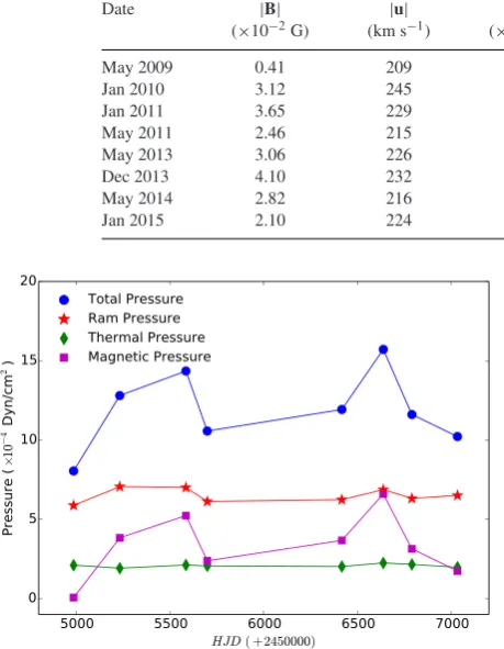
Table 4. Summary of the wind properties at the position of the planetτBoo b. The variations in absolute magnetic field,
|B|, reflects the variation in the observed field. The influence of the magnetic flux changes are seen in variations of the total pressure experienced by the planet.
Date |B| |u| T Ptot
(×10−2G) (km s−1) (×106K) (×106Particles cm−3) (×10−3dyn cm−2)
May 2009 0.41 209 1.05 1.46 0.81
Jan 2010 3.12 245 1.04 1.33 1.28
Jan 2011 3.65 229 1.07 1.43 1.44
May 2011 2.46 215 1.05 1.42 1.06
May 2013 3.06 226 1.05 1.40 1.19
Dec 2013 4.10 232 1.52 1.52 1.57
May 2014 2.82 216 1.11 1.41 1.16
Jan 2015 2.10 224 1.05 1.36 1.02
Figure 3. Pressure values at the orbit of the planetτBoo b for each observed epoch. The total pressure is the sum of the ram, thermal and magnetic pres-sures. The ram and thermal pressures vary only slightly over the observed epochs, whereas the magnetic pressure varies more significantly. The lines between points are to guide the eye, and do not represent a fit to the data. the changes in total pressure are due to changes in the magnetic pressure.
4.2 Planetary magnetospheric behaviour
The external pressure around the planet can be used to infer possible behaviours of the planet’s magnetosphere. The ratio of the planetary
magnetospheric radius,Rm, to the planetary radius,Rp, is derived from the equilibrium between the pressure from the wind and the outward force of the planetary magnetosphere. This can be written as
Rm
Rp
=
(Bp/2)2
8πPtot 1
6
(14)
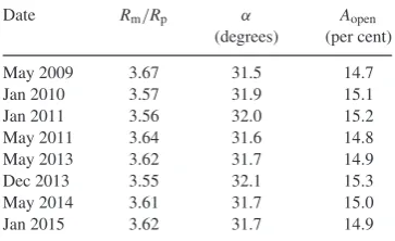
(Vidotto et al.2012),whereBpis the strength of the planetary mag-netic field at the pole. Since there have been no measurements of the magnetic field strength of hot Jupiters to date, we have assumed a planetary magnetic field strength similar to that of Jupiter, which is a maximum of∼14 G (Bagenal 1992). The values of Rm/Rp evaluated over the eight epochs are shown in Table5.
The behaviour of the planetary magnetosphere can also be de-scribed in terms of the auroral ring: the area around the poles of the planet over which the planetary magnetic flux is open, allowing the flow of particles to and from the planetary atmosphere. This can be described in terms of the percentage of the planet’s surface area:
Aopen=(1−cos(α))×100, (15)
whereαis the auroral angular aperture, defined as
α=arcsin
Rm
Rp −1
2
(16)
Vidotto et al. (in preparation).
Despite notable changes in the total pressure exerted in the planet by the star, the planet’s magnetosphere remains around 3.6 times the planet’s radius, varying by only∼3 per cent over the observed epochs. This is due to the relative insensitivity ofRm/Rpto changes
at University of Southern Queensland on May 3, 2016
http://mnras.oxfordjournals.org/
Table 5. Values for the ratio of planet magnetospheric radius to planet radius,Rm/Rp, auroral apertureαand the
percentage coverage of the polar cap,Aopen, for the planet
τBoo b. These have been calculated assuming magnetic field strength at the pole of 14 G. Despite notable changes in the behaviour of the star’s magnetic field and in the total pressure exerted on the planet by the stellar wind, these values remain quite stable over the observed epochs.
Date Rm/Rp α Aopen
(degrees) (per cent)
May 2009 3.67 31.5 14.7
Jan 2010 3.57 31.9 15.1
Jan 2011 3.56 32.0 15.2
May 2011 3.64 31.6 14.8
May 2013 3.62 31.7 14.9
Dec 2013 3.55 32.1 15.3
May 2014 3.61 31.7 15.0
Jan 2015 3.62 31.7 14.9
inPtot(due to the−1/6 power dependence). As with the planetary magnetospheric radius, there are minimal changes in the auroral aperture and polar surface area, which remain around 32◦and 15 per cent, respectively. From this we can infer that despite considerable changes in the behaviour ofτ Boo’s magnetic field, τ Boo b’s magnetosphere remains relatively stable.
5 D I S C U S S I O N
5.1 Global wind properties
The wind simulations presented here are an advance on models that do not use observationally reconstructed magnetic fields as input, or that assume a simplified stellar magnetic field topology. The coronal base temperature and density are poorly constrained by observations, and are free parameters of our model. We chose a wind base temperature that is typical of stellar coronae, and the same base density as adopted in Vidotto et al. (2012). Out estimated mass loss rate (∼2.3×10⁻¹²M
yr−1) is within the range of previous estimates of 1.67×10⁻¹²(Stevens2005) to 6.6×10⁻¹²M
yr−1 (Cranmer & Saar 2011). Given that Sun’s corona is adequately described by the adiabatic process given by equation (6), with the indexγ=1.1 (Van Doorsselaere et al.2011), we assume the same for this star.
The behaviour of the angular momentum loss rate and associ-ated spin-down time-scales found here agree with the predictions of Gallet & Bouvier (2013), who computed rotational evolution mod-els based on wind-breaking laws derived for magnetised Solar-type stars. They find that the spin-down time-scales of stars at 1 Gyr old, which is the approximate age ofτ Boo (Borsa et al.2015), should converge to the length of a few Gyrs, the same as presented in the results here. This further strengthens our choice of model parameters.
The lifetime of a main-sequence star,τMS, with the mass ofτBoo (1.34 M) is expected to be∼4.8 Gyr (τMS=10(M∗/M)−2.5).
Givenτ Boo‘s estimated age of 1 Gyr and our calculated mean spin-down time of∼4.9 Gyr, this implies that Tau Boo will remain a rapid rotator throughout its main sequence lifetime, provided that only the stellar wind is affecting its rotational evolution.
The changing stellar magnetic field polarity of the poles does not have an effect on the wind solution. This is because there is no preferred up or down orientation of the star, and the global wind
properties are calculated as surface integrals around the star. Instead, it is the changing field strength as the star undergoes its reversals that drives changes in the wind behaviour.
Over the cycle there is a change in field complexity, and this is anti-correlated with on the fraction of open fluxfopen(linear correla-tion coefficient= −0.72). As the field becomes more complex, the amount of flux contained in closed lines increases and the fraction of open flux decreases (see also Lang et al.2012). No correlation is found, however, between changes in field complexity and changes, or lack there of, in the angular momentum or mass loss rates.
5.2 Wind–planet interaction
Wind simulations can give insight into the potential behaviour of the planetary magnetosphere in the presence of the stellar wind. Since there have been no observations of magnetic fields of exoplanets to date, assumptions must be made as to what magnetic field can be expected fromτBoo b. There is much discussion over the possible magnetic fields of exoplanets. It has been theorized that close in hot-Jupiters such asτ Boo b are thought to have a weaker mag-netic field than similar planets further away from the host star due to the tidal locking slowing the planet’s rotation, and hence reduc-ing its magnetic field (Grießmeier et al.2004). However, there are some studies that indicate that planetary rotation does not directly influence the strength of a planet’s magnetic field (Christensen, Holzwarth & Reiners2009), but plays a role in the field geometry (Zuluaga & Cuartas2012). Given the uncertainty in hot-Jupiters magnetic fields and the similar nature of this planet to Jupiter, we have assumed a Jovian planetary magnetic field strength for this work. The resulting magnetosphere suggests the planet is protected from the stellar wind, despite large changes in the magnetic field and wind strengths over the cycle.
The minimum field strength required to sustain a magnetosphere above the surface ofτ Boo b (i.e.Rm >Rp) can be estimated by examining the condition of the space weather environment during at the most extreme part of the magnetic cycle (i.e., whenPtotis at a maximum). This is calculated to be∼0.4 G. This does not mean, however, that the planet is protected at this point, as at this limit the Auroral aperture reaches 90 degrees, exposing 100 per cent of the planets surface area to particle inflow and outflow. If we were to call a planet ‘protected’ provided less than 25 per cent of its surface area was contained within the auroral aperture, then the minimum magnetic field strength to achieve this is∼4.7 G for theτ Boo system.
6 S U M M A RY A N D C O N C L U S I O N S
This study examines the variability in the wind behaviour of the starτBoo over eight epochs from May 2009 to January 2015 - the most extensive monitoring of the wind behaviour of a single object to date (apart from the Sun). The winds are examined globally to study the star’s rotational evolution, and locally aroundτ Boo b for the possible impacts the wind might have on the planet’s magnetosphere.
Despite significant changes in the magnetic field behaviour, the mass loss rates do not significantly vary from epoch to epoch (∼4 per cent), remaining around 2.3×10⁻¹² M
yr−1. However, the angular momentum loss rate is observed to change considerably over the eight observations, ranging from 1.3×1032to 3.0×1032 erg. These findings are consistent with angular momentum loss rates and associated spin-down time-scales predicted by stellar evolution models.
at University of Southern Queensland on May 3, 2016
http://mnras.oxfordjournals.org/
1914
B. A. Nicholson et al.
Examining the wind environment of the planet shows that vari-ations in the absolute flux due to changes in the magnetic field behaviour of the star are reflected in changes in the local space weather of τ Boo b. Despite these changes, the magnetosphere from an assumed Jupiter-like planetary magnetic field is relatively invariant over the observed epochs, with the magnetospheric radius remaining around 3.6 times the size of the planetary radius.
AC K N OW L E D G E M E N T S
This work was partly funded through the University of Southern Queensland Strategic Research Fund Starwinds Project. Some of the simulations presented in this paper were computed on the Univer-sity of Southern Queensland’s High Performance Computer. This research has made use of NASA’s Astrophysics Data System. This work was carried out using theBATS-R-UStools developed at The University of Michigan Center for Space Environment Modeling (CSEM) and made available through the NASA Community Co-ordinated Modeling Center (CCMC). This work was supported by a grant from the Swiss National Supercomputing Centre (CSCS) under project ID s516. AAV acknowledges support from the Swiss National Science Foundation through an Ambizione Fellowship. Many thanks to Florian Gallet for providing the moment of inertia values for this work, and many thanks also to Colin Folsom for his help and advice.
R E F E R E N C E S
Adams F. C., 2011, ApJ, 730, 27
Bagenal F., 1992, Annu. Rev. Earth Planet. Sci., 20, 289
Baraffe I., Chabrier G., Allard F., Hauschildt P. H., 1998, A&A, 337, 403 Borsa F. et al., 2015, A&A, 578, A64
Bouvier J., 2013, EAS Publ. Ser., 62, 143
Brogi M., Snellen I. A. G., de Kok R. J., Albrecht S., Birkby J., de Mooij E. J. W., 2012, Nature, 486, 502
Catala C., Donati J. F., Shkolnik E., Bohlender D., Alecian E., 2007, MNRAS, 374, L42
Christensen U. R., Holzwarth V., Reiners A., 2009, Nature, 457, 167 Cranmer S. R., Saar S. H., 2011, ApJ, 741, 54
Donati J. F., Landstreet J. D., 2009, ARA&A, 47, 333 Donati J. F. et al., 2006, MNRAS, 370, 629 Donati J. F. et al., 2008, MNRAS, 385, 1179 Fares R. et al., 2009, MNRAS, 398, 1383
Fares R., Moutou C., Donati J.-F., Catala C., Shkolnik E. L., Jardine M. M., Cameron A. C., Deleuil M., 2013, MNRAS, 435, 1451
Gallet F., Bouvier J., 2013, A&A, 556, A36 Grießmeier J. M. et al., 2004, A&A, 425, 753 Horner J., Jones B. W., 2010, Int. J. Astrobiol., 9, 273
Jardine M., Vidotto A. A., van Ballegooijen A., Donati J. F., Morin J., Fares R., Gombosi T. I., 2013, MNRAS, 431, 528
Lammer H. et al., 2012, Earth Planets Space, 64, 179
Lang P., Jardine M., Donati J.-F., Morin J., Vidotto A., 2012, MNRAS, 424, 1077
Llama J., Vidotto A. A., Jardine M., Wood K., Fares R., Gombosi T. I., 2013, MNRAS, 436, 2179
Lundin R., Lammer H., Ribas I., 2007, Space Sci. Rev., 129, 245 Marsden S. C. et al., 2014, MNRAS, 444, 3517
Mengel M. W., Fares R., Marsden S. C., Carter B. D., Jeffers S. V., Folsom C. P., 2016, MNRAS, in press
Mestel L., 1999, Stellar Magnetism, Oxford Univ. Press, Oxford Poppenhaeger K., Wolk S. J., 2014, A&A, 565, L1
Poppenhaeger K., G¨unther H. M., Schmitt J. H. M. M., 2012, Astron. Nachr., 333, 26
Powell K. G., Roe P. L., Linde T. J., Gombosi T. I., De Zeeuw D. L., 1999, J. Comput. Phys., 154, 284
Schatzman E., 1962, Annales d’Astrophysique, 25, 18 Stevens I. R., 2005, MNRAS, 356, 1053
Takeda G., Ford E. B., Sills A., Rasio F. A., Fischer D. A., Valenti J. A., 2007, ApJS, 168, 297
T´oth G. et al., 2012, J. Comput. Phys., 231, 870
Van Doorsselaere T., Wardle N., Del Zanna G., Jansari K., Verwichte E., Nakariakov V. M., 2011, ApJ, 727, L32
Vidotto A. A., Fares R., Jardine M., Donati J. F., Opher M., Moutou C., Catala C., Gombosi T. I., 2012, MNRAS, 423, 3285
Vidotto A. A., Jardine M., Morin J., Donati J. F., Lang P., Russell A. J. B., 2013, A&A, 557, 67
Vidotto A. A., Jardine M., Morin J., Donati J. F., Opher M., Gombosi T. I., 2014, MNRAS, 438, 1162
Weber E. J., Davis L., Jr, 1967, ApJ, 148, 217
Wood B. E., Linsky J. L., G¨udel M., 2015, in Lammer H., Khodachenko M., eds, Astrophysics and Space Science Library Vol. 411, Astrophysics and Space Science Library. p. 19
Zuluaga J. I., Cuartas P. A., 2012, Icarus, 217, 88
A P P E N D I X A : S E N S I T I V I T Y O F R E S U LT S T O G R I D R E F I N E M E N T L E V E L
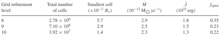
The design of theBATS-R-UScode allows the simulation grid to be constructed so that areas of interest can be studied in greater detail by local grid refinement. This means that the region closest to the surface of the star that is changing the greatest can be simulated at a much finer resolution, but leaving the outer regions of the simulation with a much coarser grid structure to save on computing resources. This section examines how the level of refinement of the grid, that is, the number of times the grid in the region close to the star is subdivided into smaller cells, affects the simulation outcomes. Using the May 2011 data, we examined ˙M, ˙J andfopen(as calcu-lated in Section 3.2) for three different refinement levels. TableA1
shows these global wind parameters, along with the total number of computational cells and smallest cell size for each refinement level. In our grid design, the grid refinement changes occur in the simulation region close to the surface of the star, so that the grid size out beyond 10R∗remains the same.
[image:8.595.113.476.669.731.2]The values of the wind parameters are seen to vary across re-finement levels, and these variations are on the same order as the variations observed across epochs, or greater as in the case of mass loss rate. However, these variations are much smaller than the
Table A1. This table shows the changes in the May 2011 global wind parameters with differing grid refinement levels. These variations are on similar to or greater than the variation between epochs. As such it is important to ensure that the grid levels are the same when comparing global wind properties between simulations.
Grid refinement Total number Smallest cell M˙ J˙ fopen
level of cells (×10−2R
∗) (10−12M
yr−1) (1032erg)
8 2.78×10⁶ 5.7 2.9 1.8 0.35
9 7.10×10⁶ 2.9 2.5 1.5 0.23
10 3.92×10⁷ 1.4 2.3 1.3 0.22
at University of Southern Queensland on May 3, 2016
http://mnras.oxfordjournals.org/
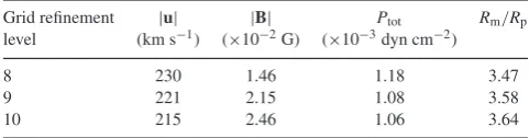
Table A2. This table shows the changes in the May 2011 local wind envi-ronment aroundτBoo b with differing grid refinement levels. The variation in due to grid refinement level is on the same level or greater than the vari-ation epoch to epoch. As such it is important to ensure that the grid levels are the same when comparing wind models across epochs.
Grid refinement |u| |B| Ptot Rm/Rp
level (km s−1) (×10−2G) (×10−3dyn cm−2)
8 230 1.46 1.18 3.47
9 221 2.15 1.08 3.58
10 215 2.46 1.06 3.64
observational uncertainties and theoretical limits of both ˙M and ˙
J. The changes infopenare not unexpected as the finer cell structure means that more of the magnetic field structure is being resolved, and field lines that could be taken to be open in a coarser grid structure are found to be closed at a higher refinement level.
TableA2shows the changes in the simulation results at the po-sition ofτ Boo b due to changes in grid refinement. As with the global wind properties, the local wind properties at the planet vary between grid sizes on the same scale as variations between epochs. Even though it might appear that an under-resolved grid overes-timates the impact of the wind on the planet, these variations are smaller than the observational uncertainties on these parameters.
Given the variations seen due to different grid sizes it is impor-tant to use the same grid refinement level to compare simulations of different epochs. Using a higher resolution would give marginally more accurate results, but given the unreasonable amount for com-putation requires to reach refinement level 11 (total number of cells
∼2.86×10⁸), we conclude that refinement level 10 is the most appropriate for the current study.
This paper has been typeset from a TEX/LATEX file prepared by the author.
at University of Southern Queensland on May 3, 2016
http://mnras.oxfordjournals.org/