1-1-2015
Estimating the Value of Conjunctive Water Use at a
System-Level Using Nonlinear Programing Model
Duc-Anh An-VoComputational Engineering and Science Research Centre, University of Southern Queensland
Shahbaz Mushtaq
International Centre for Applied Climate Science, University of Southern Queensland
Kathryn Reardon-Smith
International Centre for Applied Climate Science, University of Southern Queensland,
Follow this and additional works at:http://epubs.scu.edu.au/jesp
Part of theAgribusiness Commons,Other Applied Mathematics Commons, and theOther Engineering Commons
ePublications@SCU is an electronic repository administered by Southern Cross University Library. Its goal is to capture and preserve the intellectual output of Southern Cross University authors and researchers, and to increase visibility and impact through open access to researchers around the Recommended Citation
An-Vo, Duc-Anh; Mushtaq, Shahbaz; and Reardon-Smith, Kathryn (2015) "Estimating the Value of Conjunctive Water Use at a System-Level Using Nonlinear Programing Model,"Journal of Economic and Social Policy: Vol. 17 : Iss. 2 , Article 9.
and harvesting regimes, necessitate development of groundwater in many irrigation management areas. Groundwater can be expensive to pump, but provides a reliable supply if managed sustainably. Groundwater can be used optimally in conjunction with surface water supplies. The use of such conjunctive systems can significantly decrease the risk associated with a stochastic availability of surface water supply.
We propose an innovative nonlinear programing model for the optimisation of profitability and productivity in an irrigation command area with conjunctive water use options. The model, rather than using exogenous yields and gross margins, uses crop water production and profit functions to endogenously determine yields and water use, and associated gross margins, respectively, for various conjunctive water use options. The model allows the estimation of the potential economic benefits of conjunctive water use and derives an optimal use of regional level land and water resources by maximising the net benefits and water productivity under various physical and economic constraints.
The proposed model is applied to the Coleambally Irrigation Area (CIA) in south eastern Australia to explore potential economic benefit of conjunctive water use. The results show that optimal conjunctive water use can offer significant economic benefit, especially at low levels of surface water allocation and pumping cost. At lower levels of surface water allocation the results show that conjunctive water use potentially generate additional AUD 57.3 million. On the other hand, at higher levels of surface water allocation, additional benefit of conjunctive water use is AUD 9.4 million. The model could be applied to analyse the impact of escalating energy prices for groundwater dependent irrigation systems, and other irrigation systems, to maximise the potential of conjunctive water use.
Keywords
Surface water, groundwater, conjunctive water use model, agricultural production and profit functions, optimal multicrop production
Cover Page Footnote
1.
Introduction
Water is the most important input in irrigated agriculture, with timely and reliable supply being a major determinant in cropping decisions (Khan, Yuanlai and Blackwell, 2006). Irrigators, however, often have to make key decisions on crop acreage and input investments in the absence of reliable information on water availability. This is especially the case with surface water resources which depend upon rainfall and water stored in reservoirs. Climate change and climate variability make seasonal rainfall less predictable and seasonal irrigation supplies more uncertain, potentially eroding agricultural production and farming profitability. Uncertain surface water allocations also deter irrigators from making long-term investments or entering into seasonal water trading and insurance contracts (Dwyer, Loke, Appels, Stone and Peterson, 2005). In addition to the stressors of climate variability, new urban, industrial, and environmental water demands have priority for water allocation over agriculture, and are thus putting even further strain on the ever dwindling water resources available to farmers (Ward, Booker and Michelsen, 2006; Wichelns and Oster, 2006).
Development of optimum land uses and water allocation plans and operable water delivery schedules are valuable for irrigation schemes in arid and semi-arid regions. Surface water usually has low delivery and extraction costs, but is subject to high variability in supply. Uncertainty and shortages of surface water supplies necessitate development of groundwater in many irrigation management areas. While groundwater can be expensive to pump, it may provide a reliable supply where managed sustainably. Groundwater can be used optimally in conjunction with surface water supplies. Such conjunctive use systems can significantly decrease the risk associated with a stochastic availability of surface water supply and safeguard against risks of losing investment (Gemma and Tsur, 2007; Tsur and Graham-Tomasi, 1991).
The innovation of our approach is the use of production and profit functions to estimate agricultural yields and gross margins, respectively, for various surface water allocation levels and conjunctive water use options. The present approach differs from the commonly used method based on given crop yields and gross margins. The model endogenously determines suitable levels of water uses and associated optimal production for a given water availability and maximises net return. Another key feature of the model is that it allows water trading (buy/selling) to maximise the net benefit.
The specific objectives of the present study are to develop a mathematical programmingmodel to explore the economic potential of conjunctive water use options, and to achievean optimal use of water resources by maximising net benefits and water productivity under various physical and economic constraints. The proposed model isapplied to the Coleambally Irrigation Area (CIA) in south eastern Australia.
2.
Model formulation
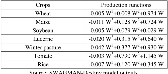
We model yields and gross margins under various water allocation levels and conjunctive water use options using production and profit functions, rather than using exogenous crop yields and gross margins. Production functions represent the yield of main crops in response to water use and are estimated using yearly rainfall data and applied irrigation of specified amounts at set dates during the growing period. Given total water inputs, i.e. irrigation plusrainfall, crop yield production functions are derived for various crops using the SWAGMAN-Destiny model (Edraki, Smith, Humphreys, Khan, O’Connell and Xevi, 2003). Developed production functions are obtained by fitting the followingnonlinear curve using ordinary least squares (OLS) regression analysis:
ε β
β β
β + + − +
= 0 1 2 2 3 3
)
(W W W W
Y (1)
where Y is the yield (tonne per ha), W is the water use (ML per ha), βi (i =0, 1, 2, 3) are coefficients and ε is the error term.
The profit function of a crop represents the net return after subtracting the input cost and water cost from the output revenue of that crop, i.e.
[
p W p W]
X XC X W Y p X W
price (AUD per ML); p(g) is the groundwater pumping cost (AUD per ML); and
) (s
W and W(g) are surface and groundwater uses of a crop, respectively. We have:
) (s
W W(g) 3
The total gross margin (TGM) denoted by Π for crop production and water trading
of the whole farming business is calculated as
Π , 4
where i is the crop index of a crop grown in the farm; is the temporary water
trading price (AUD per ML); and and are the quantities of surface water and groundwater trading, buying when , < 0 or selling when
, > 0 (in ML).
A nonlinear programming (NLP) model is generated here with the aim of maximising the TGM in (4) subject to several land, water, technical and administrative constraints. The model is represented in the form of vector functions as follows.
maximise Π xxxx xxxx !"
subject to )xxxx 0, + ,
)xxxx - 0, + ..
(5)
It can be seen that the objective function f(x) represents the right hand side of (4) with x being a vector of the input variables including the surface and groundwater use and area of each crop and the quantities of trading water. The functions ci(x), i = 1, 2. . . n are additional constraint functions, and E and I are the index sets of equality and inequality constraints, respectively. In the present work, the objective function is a nonlinear function while the constraint functions can be either linear or nonlinear. More details about the constraint functions are given below:
Surface water constraint
Total surface water use must not exceed the corresponding announced water allocation for the water year, as shown below:
where is the crop surface water use (ML per ha) of crop i, SW is the total surface water entitlement for an irrigation system, and A is the surface water allocation (%) in a given month.
Groundwater constraint
Groundwater licenses/withdrawal of water should not exceed the maximum sustainable yield,as represented through
0 45
7
where is the crop groundwater use (ML per ha) of crop i, GW(sy) is the sustainable groundwater, based on the extraction limit.
Land constraint
Land allocated to various crops must not exceed the total cultivable area during the summer and winter seasons, i.e.
0 72
8
where TA is the total cultivated area available.
Allowable area constraints
Management considerations, market conditions, machinery capacity of the farm, and climatic conditions restrict the minimum or maximum land acreages for certain crops such as rice to meet the regulations on local land use in the area. For instance
(a) Lower bound - 9:"72 9
(b) Upper bound 0 9:<=72 10
where 9:"and 9:<= are minimum and maximum fractions, respectively, of the cultivated area under crop i.
Water market constraint
0 ?:<=1 2 10
where ?:<= is a fraction of the total allocation that can be traded on temporary water markets.
Non-negativity constraints
The non-negativity constraints which ensure the solution remains feasible are given as follows.
- 0. 12
A sequential quadratic programming (SQP) technique is used to solve the mathematical model (5). SQP methods represent the state of the art in nonlinear programming. Schittkowski (Schittkowski, 1985), for example, has implemented and tested a version that outperforms every other tested method in terms of efficiency, accuracy, and percentage of successful solutions, over a large number of test problems. The SQP technique achieves the solution of a constrained nonlinear programming problem via sequentially solving quadratic programming subproblems in which the nonlinear constraints are linearized (Fletcher, 1991). Computer codes for the SQP algorithm are written in MATLAB® language.
3.
Application example
[image:7.612.160.456.477.662.2]The developed model is generally valid and its application has allowed an estimate of the benefits of conjunctive water use for the Coleambally Irrigation Area (CIA), a major irrigated agricultural region located in the Murray-Darling Basin (MDB) in the south eastern New South Wales (Figure 1).
3.1Irrigation command area
3.1.1 Surface water
Surface water for the CIA is stored in Burrinjuck and Blowering dams and is diverted to the area via the Murrumbidgee River at the Gogeldrie Weir. CIA irrigation system consists of 41 km of main canal from the Murrumbidgee River, 477 km of supply channels, and a further 734 km of drainage channels. Coleambally Irrigation Cooperative Limited (CICL) is a leading exponent of open channel irrigation management and has invested over AUD 40 million since 2000 improving their land and water management practices and enhancing local biodiversity. Rainfall in the CIA is in the range of 400-450 mm per year. There are over 360 landholdings with a total area of 79 000 ha, and a total bulk water license of 629 GL. Prolonged drought severely impacts water availability; for example, surface water deliveries declined significantly from 629 GL in 1996/1997 to 36 GL in 2007/2008 and increased to 427 GL in 2011/2012 following good seasonal rains (Figure 2).
Available surface water suppliesare allocated on a priority basis; first to high security water and then to general security water. High security consumptive water licenses include town water supplies and permanentcrops (e.g. tree crops). Irrigators with high security water usually receive close to full entitlement (e.g. at 95% allocation during 2005/2006). General security water licenses represent most of the CIA’s farming business. The first irrigation allocation announcement for general security water users in the CIA is at the beginning of the irrigation season around July-August. This announcement is usually conservative based on a high level of reliability (i.e. that there is a 99% chance that the announced allocation will be available). General security allocations build gradually over the irrigation season as inflows into storages andrivers occur. Figure 3 shows the trend in the general security allocation for the period, July-December 2011.
3.1.2 Groundwater
Figure 2: Annual diversion in the CIA
Figure 3: Announced allocation of the CIA for the period, 1 July 2011
December 2011 (CICL, 2012)
Annual diversion in the CIA (CICL, 2012).
Announced allocation of the CIA for the period, 1 July 2011 (CICL, 2012).
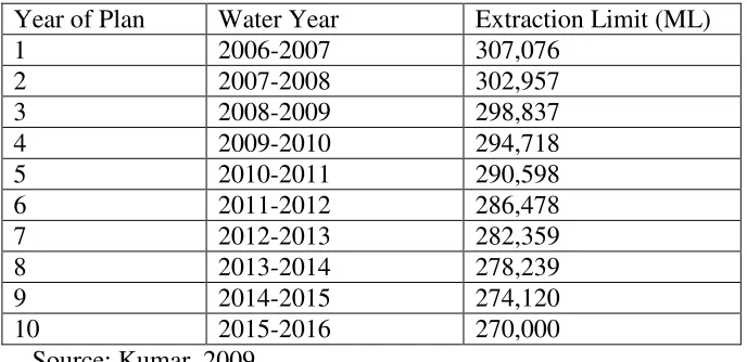
[image:9.612.131.477.387.602.2]Groundwater management policy for the region has been developed since 1955 starting with all water bores constructed requiring a license. Licences were issued in perpetuity with no area or volume based restrictions until 1984 when the volumetric allocation basis was introduced. The annual groundwater entitlement was increased gradually from 147 GL in 1983/1984 to a peak amount of 529 GL in 2000/2001 (Kumar, 2002). In 2003, a 10-year water sharing plan (the Plan) for groundwater sources was developed. The Plan uses the average annual groundwater recharge of about 400 GL as the basis for sharing water between extractive users and the environment. It provides for a portion of the estimated recharge to be reserved for the environment allowing the remainder to be available for extraction. The Plan was implemented in 2006 with total entitlements reduced from 307 GL to the target of 270 GL in 2015/2016. Table 1 presents the annual extraction limits of groundwater for the ten years of the Plan from 2006-2016.
[image:10.612.135.479.341.508.2]
Table 1: The Plan of annual extraction limits for CIA groundwater source
Year of Plan Water Year Extraction Limit (ML)
1 2006-2007 307,076
2 2007-2008 302,957
3 2008-2009 298,837
4 2009-2010 294,718
5 2010-2011 290,598
6 2011-2012 286,478
7 2012-2013 282,359
8 2013-2014 278,239
9 2014-2015 274,120
10 2015-2016 270,000
Source: Kumar, 2009.
3.1.3 Land and water use
pre-2002/03 levels. The areas committed to the production of soybeans, corn, wheat, pasture and canola have varied greatly over the last five years in response to the availability of water and changes in commodity prices.
3.2Model application
We modeled productivity in CIA for seven crops including wheat, maize, soybean, pasture, lucerne, rice and tomato. More crops can be added to the model straightforwardly, if required. The production functions for the main crops in CIA (Table 3) were developed using the yearly rainfall data for Griffith for the last 30 years. The total cultivated area available (TA) is the total area of CIA (79 000 ha). The total surface water entitlement (SW) is 629 GL, the total bulk water license. The sustainable groundwater volume GW(sy) is set as the extraction limits before and after the Plan. A typical value of 471 GL is used as the extraction limit before the Plan while the extraction limits of the Plan are as given in Table 1.
The value of temporary traded water was estimated using a regression model involving the monthly average water trade price and water allocation data from the years 2001/2002 to 2005/2006. The resulting high R2 value (0.93) indicates that water allocation is the key factor determining the water market price. The following estimated function was used in the application of the model:
407.72 A 10.172 0.072B 13
[image:11.612.72.547.494.682.2]where A is the general security water allocation (%) in a given month.
Table 2: Land area and consumptive water use of main crops in the CIA
Source: CICL, 2013. Crops
2008/09 2009/10 2010/11 2011/12 2012/13 Land use (ha) Water use (%) Land use (ha) Water use (%) Land use (ha) Water use (%) Land use (ha) Water use (%) Land use (ha) Water use (%) Rice 2135 33.1 3668 46 14512 68.3 16745 62.1 19071 52.7 Corn/Maize 2472 3.4 311 2 4367 7.2 4767 8.2 4872 7.7
Table 3: Estimated water yield production functions for the main crops in CIA
4.
Results
The optimisation model, in general, is assumed to have a short term focus and is estimated under the assumption of a relevant output price range and relatively inelastic demand for water. Over the years 2008–2012 the average price of surface water including fixed and variable charges was AUD 35.65 per ML.
It is desirable when dealing with optimisation problems that the global optimum be found. To search for the global rather than local optimum, we used the median values of crop water use as starting values. Average crop water use can be found in (CICL, 2013).
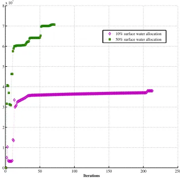
Figure 4 displays the convergence behaviour of the algorithm applied to the present NLP model at two surface water allocation levels. It can be seen that the algorithm converges well to the maximum value of the objective function after about 210 and 70 iterations at 10% and 50% surface water allocation, respectively. At a certain surface water allocation level, the NLP model is firstly run with surface water use only (groundwater extraction limit is set to zero) to obtain the corresponding total gross margin (TGM) of surface water use. We then run the model with conjunctive water use by setting the groundwater extraction limit to the values before and after the Plan. The additional economic benefit of groundwater (“conjunctive benefit”) owing to conjunctive water use is defined as the difference between the TGM of conjunctive water use and the TGM of surface water use only:
Figure 4: Convergence behaviour of the SQP algorithm applied to the present NLP model
Conjunctive benefit=TGMconjunctive water - TGMsurface water 15
Table 4 and 5 shows the economic benefit of conjunctive water use at different surface water allocation levels for two scenarios of groundwater price i.e.
) ( )
(g s
p
p = and (g) 2 (s) p
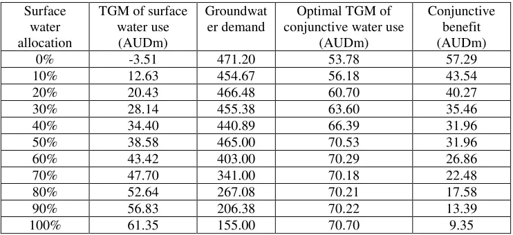
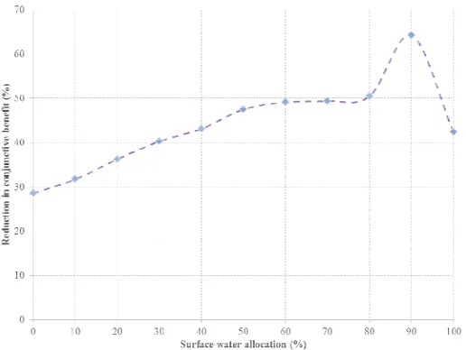
p = , respectively. Table 5 presents the results for the case of 100% increase of groundwater price compared to the groundwater price used to obtain the results in Table 4. The increase of groundwater price here is assumed due to the projected increase in energy price but not due to the dynamic of groundwater table which will be considered in future work with a dynamic model being developed. As expected, the conjunctive benefit is high at lower levels of surface water allocation compared to those at higher levels of allocation. The maximum benefit appears at 0% surface water allocation with a negative value for the TGM of surface water use. The negative TGM is a result of the area constraint requiring the farmer to buy water at a high price for growing certain compulsory crops. The use of groundwater at 0% surface water allocation can potentially result in maximum economic benefit of AUD 57.29 and AUD 40.92 million, respectively, for the two cases of groundwater price while minimum benefit of AUD 9.35 and AUD 4.79 million appears at 100% and 90% surface water allocation, respectively, in the two cases. The conjunctive benefit in Table 5 shows significant reductions compared to those in Table 4 when the groundwater price is increased by 100%. The reductions (%) of conjunctive benefit at different surface water allocation levels are presented in Figure 5 where a maximum reduction of 65% appears at 90% allocation. Groundwater demand reduces from
0 50 100 150 200 250
0 1 2 3 4 5 6 7 8x 10
7
Iterations
Function values
[image:13.612.220.402.117.297.2]the groundwater extraction limit at 0% surface water allocation to 155 GL and 158 GL, respectively, at 100% allocation. In contrast to the conjunctive benefit, the total gross margin of conjunctive water use in the first scenario (Table 4) firstly increases as the surface water allocation increases to 50% allocation then becomes numerically flat. For the second scenario (Table 5) the TGM increases as the surface water allocation increases. The TGM trends result in a difference of greater than 50% allocation between the two scenarios, probably due to the contribution of surface water to TGM which is more significant in the second scenario where the groundwater price is high.
Table 4: Economic benefit of conjunctive water use for different levels of surface
water allocations with (g) (s) p
p =
Surface water allocation
TGM of surface water use
(AUDm)
Groundwat er demand
Optimal TGM of conjunctive water use
(AUDm)
Conjunctive benefit (AUDm)
0% -3.51 471.20 53.78 57.29
10% 12.63 454.67 56.18 43.54
20% 20.43 466.48 60.70 40.27
30% 28.14 455.38 63.60 35.46
40% 34.40 440.89 66.39 31.96
50% 38.58 465.00 70.53 31.96
60% 43.42 403.00 70.29 26.86
70% 47.70 341.00 70.18 22.48
80% 52.64 267.08 70.21 17.58
90% 56.83 206.38 70.22 13.39
100% 61.35 155.00 70.70 9.35
Table 5: Economic benefit of conjunctive water use for different levels of surface
water allocations withp(g) =2p(s)
Surface water allocation
TGM of surface water use
(AUDm)
Groundwat er demand
Optimal TGM of conjunctive water use
(AUDm)
Conjunctive benefit (AUDm)
0% -3.51 471.20 37.41 40.92
10% 12.63 471.20 42.35 29.72
20% 20.43 471.20 46.10 25.67
30% 28.14 471.20 49.31 21.17
40% 34.40 471.20 52.58 18.18
50% 38.58 467.64 55.36 16.78
60% 43.42 405.64 57.08 13.66
70% 47.70 343.64 59.07 11.37
80% 52.64 281.64 61.35 8.71
90% 56.83 148.04 61.62 4.79
[image:14.612.120.492.513.684.2]Figure 5: Reduction in economic benefit of conju groundwater price increases by 100%
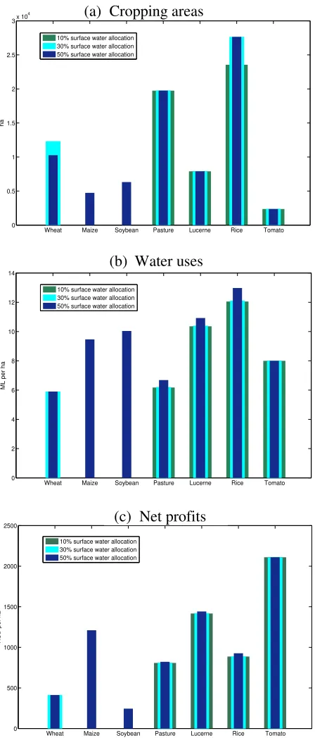
Figure 6 shows the proposed optimal cropping areas, associated water use and net profit of the seven crops at 10%, 30% and 50% allocations, yielding TGMs of AUD 56.18, 63.60 and 70.53 million, respectively
allocation, due to the shortage of surface water resources farmers make a tactical decision to grow crops with high net profits and the total cr
to 53,54 ha which is smaller than the available cropping area in the CIA. The average profit for cropping land
990 per ha. In contrast, at 50% allocation, farmers have enough water resources to grow all crops on the 79,000 ha of available cropping area. The average profit for cropping land for this scena
even though the net profit of maize might be high compared to wheat as shown in the case of 50% allocation (Figure 6c
allocation is zero due to the area constraint betw
6a). The area constraint also results in the area of soybean exceeding that of maize in the case of 50% allocation (Figure 6a
use requirement (Figure 6b
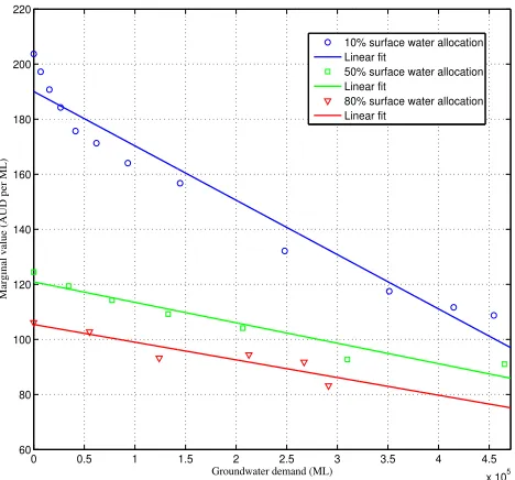
Figure 7 presents the marginal value of groundwater and its linear fitting lines for three levels of surface water allocation
agreement with expectation as the derived willingness to pay for the groundwater increases as the surface water allocation decreases. In each surface water allocation level, the groundwater marginal value decreases as the groundwater demand increases.
Reduction in economic benefit of conjunctive water use when groundwater price increases by 100%.
shows the proposed optimal cropping areas, associated water use and net profit of the seven crops at 10%, 30% and 50% allocations, yielding TGMs of AUD 56.18, 63.60 and 70.53 million, respectively, with (g) (s)
p
p = . At 10% e shortage of surface water resources farmers make a tactical decision to grow crops with high net profits and the total cropping area is reduced ha which is smaller than the available cropping area in the CIA. The average profit for cropping land is high in this case and is estimated to be AUD per ha. In contrast, at 50% allocation, farmers have enough water resources to grow all crops on the 79,000 ha of available cropping area. The average profit for cropping land for this scenario is estimated to be AUD 883 per ha. It is noted that even though the net profit of maize might be high compared to wheat as shown in ase of 50% allocation (Figure 6c) the cropping area of maize at 30% allocation is zero due to the area constraint between maize and soybean (Figure ). The area constraint also results in the area of soybean exceeding that of maize
ase of 50% allocation (Figure 6a) even though soybean has a higher use requirement (Figure 6b) and yields lower net profit (Figure 6c).
presents the marginal value of groundwater and its linear fitting lines for three levels of surface water allocation with p(g) = p(s). The lines are in agreement with expectation as the derived willingness to pay for the groundwater creases as the surface water allocation decreases. In each surface water allocation level, the groundwater marginal value decreases as the groundwater
ctive water use when
shows the proposed optimal cropping areas, associated water use and net profit of the seven crops at 10%, 30% and 50% allocations, yielding TGMs of . At 10% e shortage of surface water resources farmers make a tactical opping area is reduced ha which is smaller than the available cropping area in the CIA. The and is estimated to be AUD per ha. In contrast, at 50% allocation, farmers have enough water resources to grow all crops on the 79,000 ha of available cropping area. The average profit for per ha. It is noted that even though the net profit of maize might be high compared to wheat as shown in ) the cropping area of maize at 30% and soybean (Figure ). The area constraint also results in the area of soybean exceeding that of maize ) even though soybean has a higher water
Figure 6: (g) (s) p
p = : proposed optimal cropping areas (a), associated water use (b) and net profits (c) of the seven crops at 10%, 30% and 50% surface water allocations
Wheat Maize Soybean Pasture Lucerne Rice Tomato 0
0.5 1 1.5 2 2.5
3x 10 4
ha
t
10% surface water allocation 30% surface water allocation 50% surface water allocation
Wheat Maize Soybean Pasture Lucerne Rice Tomato 0
2 4 6 8 10 12 14
t
ML per ha
10% surface water allocation 30% surface water allocation 50% surface water allocation
Wheat Maize Soybean Pasture Lucerne Rice Tomato 0
500 1000 1500 2000
2500 t
AUD per ha
10% surface water allocation 30% surface water allocation 50% surface water allocation
(a) Cropping areas
(b) Water uses
Figure 7: p(g) = p(s): groundwater demand lines for three levels (10%, 30% and 50%) of surface water allocation
5. Discussion
The model developed in this study can be applied to any irrigation command area to help farmers in making management decisions for irrigation and productivity in the face of the climate variability. The irrigation management capability of the model enables an optimal and sustainable volume of groundwater use to be determined for a given or projected level of surface water availability. Such capability helps reduce the risk associated with the high variability of surface water supply.
The decisions around optimising productivity (e.g. crop type, cropping area, crop water use) are endogenous outputs of the model which are valuable for farmers. As an example, in Figure 8, we compare the model results of land and water use for several crops with those reported for the CIA in the irrigation year 2011/12 (CICL, 2012). The surface water allocation is assumed to be the average surface water allocation from Figure 3 which is about 50%. It can be seen that there is a potential improvement in productivity using the model to determine optimal levels of land and water use at the regional level. Model results encourage the increase of crop areas to high value crops such as paster. In regards to potential for improved crop water uses, model results suggest potential to reduce water use
0 0.5 1 1.5 2 2.5 3 3.5 4 4.5
x 105 60
80 100 120 140 160 180 200 220
Groundwater demand (ML)
Marginal value (AUD per ML)
10% surface water allocation Linear fit
50% surface water allocation Linear fit
for rice while allocating more water to other crops such as wheat, maize and pasture to increase economic returns of the CIA irrigation system.
Figure 8: Land area (a) and water uses (b) for the CIA from the reported data for the
irrigation year 2011/2012 and from the model results at 50% surface water allocation
Rice Maize Soybeans Wheat Pasture
0 0.5 1 1.5 2 2.5
3x 10
4 t
ha
Reported data (CICL, 2012) Model results
Rice Maize Soybeans Wheat Pasture
0 0.5 1 1.5 2 2.5
3x 10
4
ML per ha
Reported data (CICL, 2012) Model results
(a) Cropping areas
[image:18.612.193.417.156.635.2]6. Conclusion and policy implications
We have developed a nonlinear programming model as an innovative tool for the optimisation of productivity in an irrigation command area with conjunctive water use. The model uses production and profit functions to estimate yield and gross margins for various water allocation levels, which is conceptually different from the commonly used approach based on given crop yields and gross margins. The model has been applied to the CIA and has been proven able to project the conjunctive water use benefit, marginal value of groundwater at different surface water allocation and groundwater demand levels. Critically, the current model can be integrated with a surface water forecasting model for the effective management of water resources in an irrigation command area such as the CIA. Though the developed model is static, the extension of this model to a more dynamic model that can capture the groundwater variability and groundwater management is our aim in future works.
With regard to the policy implication of this study, the findings suggest integrated management of surface and groundwater management to realise optimal outcomes. Particularly, this will allow to stabilising groundwater resource during high water allocation years, when marginal value of water is relatively low, and allow storing additional groundwater to provide buffer during extremely low water allocation years. Also, careful economic benefit estimation incorporating increases in energy prices and associated environmental impacts would be a key before the implementation conjunctive water management systems.
References
Chaves-Morales J., Marino M.A. and Holzapfel A.H. (1992). Planning simulation model
of irrigation district. Journal of Irrigation and Drainage Engineering, ASCE 118,
74–87.
CICL (2013). Annual Compliance Report. Coleambally Irrigation Cooperative Limited,
NSW, Australia.
CICL (2012). Annual Compliance Report. Coleambally Irrigation Cooperative Limited,
NSW, Australia.
Dwyer G., Loke P., Appels D., Stone S. and Peterson D. (2005). Integrating rural and
urban water markets in south east Australia: preliminary analysis. OECD
Workshop on Agriculture and Water: Sustainability, Markets and Policies. Adelaide.
Edraki M., Smith D., Humphreys E., Khan S., O’Connell N. and Xevi, E. (2003). Validation of the SWAGMAN farm and SWAGMAN destiny models. Technical
Report. CSIRO land and water.
Khan S., Triaq R., Yuanlai C. and Blackwell J. (2006). Can irrigation be sustainable?
Agricultural Water Management, 80, 87 – 99.
Khan S., Taiq R., Hanjra M. and Zirilli, J. (2009). Water markets and soil salinity nexus:
can minimum irrigation intensities address the issue? Agricultural Water
Management, 96, 493–503.
Kumar B.P. (2002). Review of groundwater use and groundwater behaviour in the Lower Murrumbidgee Groundwater Management Area, Groundwater report number 6.
Department of Natural Resources (DNR), NSW, Australia.
Kumar B.P. (2009). Lower Murrumbidgee groundwater resources. Technical Report.
NSW Office of Water.
Latif M. and James L.D. (1991). Conjunctive water use to control waterlogging and
salinization. Journal of Water Resources Planning and Management, ASCE 117
(6), 611–628.
Lakshminarayana V. and Rajagopalan, P. (1977). Optimal cropping pattern for basin in
India. Journal of Irrigation and Drainage Engineering, ASCE 103 (1), 53–70.
Matsukawa J., Finney B. and Willis R. (1992). Conjunctive use planning in mad river
basin, California. Journal of Water Resources Planning and Management, ASCE
118 (2), 115–132.
Gemma M., and Tsur Y. (2007). The stabilization value of groundwater and conjunctive
water management under uncertainty. Review of Agricultural Economics 29(3),
540–548
Montazar A., Riazi H. and Behbahani S.M. (2010). Conjunctive water use planning in an
irrigation command area. Water Resources Management, 24, 577–596.
Onta P.R., Gupta A.D. and Harboe, R. (1991). Multistep planning model for conjunctive
use of surface and groundwater resources. Journal of Water Resources Planning
and Management 117 (6), 662–678.
Provencher B. and Burt, O. (1994). Approximating the optimal ground water pumping
policy in a multiaquifer stochastic conjunctive use setting. Water Resources
Research 30 (3), 833–843.
Paudyal G. and Gupta A. (1990). Irrigation planning by multilevel optimization. Journal
of Irrigation and Drainage Engineering, ASCE, 116 (2), 273–291.
Rogers P. and Smith D.V. (1970). The integrated use of ground and surface water in
irrigation project planning. American Journal of Agricultural Economics 52, 13–
24.
Schittkowski K. (1985). Nlqpl: A Fortran-subroutine solving constrained nonlinear
programming problems. Annals of Operations Research 5, 485–500.
Tsur Y., and Graham-Tomasi T. (1991). The buffer value of groundwater with stochastic
surface water supplies. Journal of Environmental Economics and Management
21(20), 201-224
Ward F.A., Booker J.F. and Michelsen A.M. (2006). Integrated economic, hydrologic and
institutional analysis of policy responses to mitigate drought. Journal of Water
Resources Planning and Management, 132, 488 – 502.
Wichelns D. and Oster J.D. (2006). Sustainable irrigation is necessary and achievable, but
direct costs and environmental impacts can be substantial. Agricultural Water