Learning analytics as a tool for
exploring student learning patterns
Bethany Rognoni
BSc(Hons)
School of Agricultural, Computational and
Environmental Sciences
University of Southern Queensland
October 2017
Submitted in partial fulfillment of
the requirements of the award of
Abstract
Acknowledgements
This thesis would not have been possible without the tireless and expert guid-ance from my supervisors, Rachel King and Christine McDonald. Your support and guidance over the past two years has been amazing, from the beginning of data entry to the polishing of the final dissertation. I am so grateful for your assistance not only with the thesis itself, but also with my development of organisational and time-management skills. I now know much more about how to use R, RStudio, knitr, LATEX, and BibTEX – I never thought I could get to this level when you first offered this honours project to me two years ago. I am extremely lucky to have had the pleasure of going through this with both of you, it’s been awesome!
I am also very grateful to Enamul Kabir, Taryn Axelsen, and the markers of the statistics course that is the focus of this project, for your assistance with acquiring assessment and OLS data for this research.
Contents
1 Introduction 1
1.1 Literature Review . . . 1
1.2 Research Aims . . . 12
2 Methods 15 2.1 Structure of the course studied . . . 15
2.2 Data Collection . . . 17
2.3 Data Cleaning . . . 18
2.4 Preparation of the Data for Analyses . . . 20
2.5 Summary Statistical Methods . . . 21
2.6 Cluster Analysis . . . 22
2.7 Principal Components Analysis . . . 25
3 Results 29 3.1 Assessment achievement . . . 29
3.2 Relationships between data sources . . . 32
3.3 Multivariate Analyses . . . 41
4 Discussion and Conclusions 51 4.1 Trends and relationships in the data . . . 52
4.2 Multivariate Methods . . . 56
4.3 Potential interventions . . . 59
4.5 Conclusions . . . 63
References 64
A Code for running analyses 71
B Semester 1 Results 77
B.1 Assessment Achievement . . . 77 B.2 Relationships between data sources . . . 78 B.3 Multivariate Analyses . . . 82
C Semester 2 Results 87
List of Figures
3.1 Distribution of overall achievement for each assessment item . . 30 3.2 Histograms of differences between assignment and exam
achieve-ment for each chosen topic (Difference = Exam – Assignment) . 30 3.3 Distribution of OLS access by study mode . . . 34 3.4 Distribution of achievement on each topic for both assignment
and exam questions by study mode . . . 38 3.5 Distribution of achievement on each topic for both assignment
and exam questions by the frequency of access to tutorial solutions 40 3.6 Silhouette Width for different numbers of clusters . . . 41 3.7 2D ordination plot of aggregate distances between cases, with
cases coloured by assigned cluster . . . 42 3.8 OLS access by cluster membership . . . 45 3.9 Individuals (left) and Variables (right) factor maps displaying
both the cases and the variable vectors against the principal components . . . 46 3.10 Coloured PCA Plot with Degree Type included as a qualitative
supplementary variable . . . 49
B.1 Distribution of overall achievement for each assessment item . . 77 B.2 Histograms of differences between assignment and exam
B.4 Distribution of achievement on each topic for both assignment and exam questions by study mode . . . 80 B.5 Distribution of achievement on each topic for both assignment
and exam questions by the frequency of access to tutorial solutions 81 B.6 Silhouette Width for different numbers of clusters . . . 82 B.7 2D ordination plot of aggregate distances between cases, with
cases coloured by assigned cluster . . . 82 B.8 OLS access by Cluster membership . . . 84 B.9 Individuals (left) and Variables (right) factor maps displaying
both the cases and the variable vectors against the principal components . . . 85 B.10 Coloured PCA Plot with Degree Type included as a qualitative
supplementary variable . . . 86
C.1 Distribution of overall achievement for each assessment item . . 87 C.2 Histograms of differences between assignment and exam
achieve-ment for each chosen topic (Difference = Exam – Assignment) . 88 C.3 Distribution of OLS access by study mode . . . 89 C.4 Distribution of achievement on each topic for both assignment
and exam questions by study mode . . . 90 C.5 Distribution of achievement on each topic for both assignment
and exam questions by the frequency of access to tutorial solutions 91 C.6 Silhouette Width for different numbers of clusters . . . 92 C.7 2D ordination plot of aggregate distances between cases, with
cases coloured by assigned cluster . . . 92 C.8 OLS access by cluster membership . . . 94 C.9 Individuals (left) and Variables (right) factor maps displaying
List of Tables
2.1 Question mapping across semesters . . . 17
3.1 p-values for testing of differences between assignment and exam scores in the three topics . . . 31 3.2 Distribution of Degree Type by Study Mode . . . 32 3.3 OLS access (percentage) for each degree type . . . 35 3.4 Frequencies of Degree Type, Study Mode and OLS Access, and
mean and standard deviation of achievement in assessment ques-tions, by Cluster . . . 44 3.5 Percentage variation explained by each principal component . . 45 3.6 Loadings of the original variables on each principal component . 46
B.1 p-values for testing of differences between assignment and exam scores in the three topics . . . 78 B.2 Distribution of Degree Type by Study Mode . . . 78 B.3 OLS access (percentage) of cohort for each degree type . . . 79 B.4 Frequencies of Degree Type, Study Mode and OLS Access, and
mean and standard deviation of achievement in assessment ques-tions, by Cluster . . . 83 B.5 Percentage variation explained by each principal component . . 84 B.6 Loadings of the original variables on each principal component . 84
C.2 Distribution of Degree Type by Study Mode . . . 88 C.3 OLS access (percentage) of cohort for each degree type . . . 89 C.4 Frequencies of Degree Type, Study Mode and OLS Access, and
Chapter 1
Introduction
Learning analytics is defined as the analysis of educational data for the pur-poses of identifying behavioural trends and understanding how students in-teract with educational material (Siemens, 2012). The potential for analytics to be used in educational contexts has increased over the past few decades along with the application of advances in technology and computing capabili-ties within education delivery. However, the field of learning analytics is still relatively young (You, 2016), with papers focused on introducing the field only being written as recently as five years ago (Siemens, 2013; Soby, 2014). Conse-quently, a generalised framework for the implementation of learning analytics has not yet been fully established. This may, in part, be because the develop-ment of such a framework requires a flexible statistical analysis technique as it is heavily dependent on the context in which it is applied (Hern´andez-Garc´ıa & Conde, 2014).
1.1
Literature Review
net-work analysis and cognitive modelling (Siemens, 2013). The overarching aim in these older fields is to link behaviour with outcomes by analysing data. This has provided a benchmark to develop applied learning analytics techniques within a defined course (or subject or unit) of educational study (Siemens, 2013).
There are many drivers that motivate current interest in learning analytics. Prior to education being offered extensively online, teacher-student interac-tions were predominantly in-person, allowing the teacher to monitor student learning behaviour and its impact on academic progression simultaneously. This analysis was often a qualitative assessment based on personal interaction and not necessarily a data driven process. Following the widespread adoption of online delivery of course content, direct contact between teacher and stu-dent is becoming less reliable as a method for assessing stustu-dent engagement and progression. The platforms used to deliver content online also automate the collection of data, aspects of online behaviour of course participants being recorded (Slade & Prinsloo, 2013). This results in the passive collection and storage of large datasets containing course/subject/unit specific information that can potentially inform educators, even in cases when direct personal con-tact with students is limited or non-existent. Clow (2013) has identified that there is an increasing push toward the collection and quantification of informa-tion, as opposed to qualitative evaluation. The quantification of some aspects of education such as learning behaviours, student achievement and teaching methods will enable effective decisions to be made regarding the operation of a course within an institution, unclouded by the potentially biased judgement coming from both learners and educators.
using statistical data reduction techniques prior to or as part of the analysis of big data to help reduce the dimensionality or size of these datasets. This has allowed the application of learning analytics to become feasible in cases where huge numbers of attributes are measured for each student (de Freitas
et al., 2015). The accessibility of these methods to educators and researchers has improved as the computational capacity needed for implementation of these methods has become readily available within education fields (Slade & Prinsloo, 2013). However, care must be taken by researchers who do not have the statistical knowledge necessary to implement, understand and interpret these methods. One major downfall in this area is that the advancements in computing ability may lead to the use of advanced statistical methods by researchers simply because they are available, resulting in improper implemen-tation of the techniques or misinterpreimplemen-tation of the results (Greller & Drachsler, 2012).
individual interactions with the course content, the potential applications of learning analytics have expanded significantly (Romero-Zaldivar et al., 2012; You, 2016), with no extra effort required by the course educators for data collection to occur.
The challenge now is how best to realise the full potential of these new and potentially large data resources. The approach commonly taken is to iden-tify trends in the data after the delivery of educational content has concluded (de Freitas et al., 2015; Strang, 2016). This is useful to educators and re-searchers, as it provides a method for identifying areas where students may tend to struggle, or may reveal modules (subsets of content) that have lower rates of interaction (Soby, 2014; Yassine et al., 2016). This analysis can then inform changes to course content or delivery for future cohorts of students. However, since OLS data is generated in real-time (that is, it is generated and accessible as soon as student interaction has occurred) there is also the po-tential for real-time analysis to inform educators about their current cohort of students and provide them with tailored feedback and interventions (Gasevic
et al., 2016). Real-time analysis does pose the additional challenge of needing to complete analyses and implement changes quickly so that the current cohort is benefited, which may require extra resources (time, people) to be allocated to this work (Romero-Zaldivaret al., 2012). Whichever approach is taken, the educator or researcher must be aware of the challenges innate to using the data itself.
et al., 2016). Developments in the data science field and the propagation of big data across many discipline areas in the last decade has stimulated the development of a range of statistical methods for dealing with large datasets (Giannakos et al., 2016). These forms of analysis may assist in overcoming initial barriers of data usability and accessibility in learning analytics (Clow, 2013). In cases where data management tools offered through the OLS are not sufficient, the educator/researcher must build a framework for the application of statistical methods specific to the data of interest.
Initially the most important records of interaction need to be identified for any application of learning analytics to allow the development of strategies for data selection and collection (Hern´andez-Garc´ıa & Conde, 2014; Serrano-Lagunaet al., 2014). This allows for more insightful analyses to be performed when starting with variables that are specifically targeted to the hypothesis (Bainbridge et al., 2015). However, when data is automatically generated by an OLS, the particular form that the database takes is decided during the creation of the OLS, and the data may not necessarily be tailored for easy use in statistical analyses. Unfortunately, as highlighted by Dringus (2012), the limitations on the data collected by a particular OLS in turn limits the educator’s or researcher’s ability to obtain a complete and accurate picture of the way students interact with the learning environment.
An important aspect of interpreting OLS data raised by Bainbridge et al. (2015) was that the selection of particular interactions for analyses should be based on a desire to understand and recognise genuine learning, rather than just collecting indications of simple participation. Nyland et al. (2016) iden-tified that “transaction-level data” offers the most detail concerning students’ interactions with content. This gives it “high validity” according to Bainbridge
con-fined in its nature. In its assessment, students were expected to complete a set number of tasks within a set workspace (Microsoft Excel), and the assessment was arranged such that transaction-level data (for example, records of time spent between attempts at each step of the problem) were feasible to collect. The study concluded that using more detailed achievement data provided a better understanding of “knowledge gaps” than overall achievement, however it is cautioned that this may not be feasible for courses with different assess-ment types. Another example by Romero-Zaldivaret al. (2012) promoted the use of a self-contained, purpose-built educational setting to observe learner be-haviour, allowing the educator or researcher to tailor the aspects of the learner behaviour recorded. Despite transaction-level data enabling a better under-standing of genuine learning, this data also tends to be the most difficult data to analyse, due to the large number of attributes being measured and the need to manipulate the data in preparation for analysis.
as highlighted earlier also requires additional investment of resources. This approach may be feasible for contexts where the number of students is small (in the Cocea & Weibelzahl (2011) study there were only 48 students), how-ever it would not be appropriate for situations where larger cohorts of students are involved. The application of learning analytics to detect trends of genuine learning often involves finding a workable balance between resource investment and useful output, and this balance becomes increasingly important as the size of the dataset increases (Gasevic et al., 2016).
Researchers must also consider which OLS records are more useful than others for the identification of associations between learner behaviour and academic success. Hu et al. (2014) aimed to implement an early warning system that could reliably detect early learning behaviours in students that were strongly related to failure later in the teaching period. The study concluded that having access to time-dependant variables (that is, variables that change over time, such as frequency of OLS access, or time spent using the OLS per week) provided a more reliable prediction of academic achievement, as opposed to static variables. It is cautioned, however, that this approach is only suitable if the OLS is the primary method of accessing course resources; if an OLS is only used as a supplement to course delivery, then time-dependent variables lose their meaning. It is vital that researchers consider the course structure, particularly how students are expected to be using particular resources, and determine from this which aspects of the OLS data are likely to be useful for analyses (Gasevicet al., 2016).
not likely to be indicators of engagement with learning materials specifically, so discretion must be used by researchers when determining the usefulness and meaning of this data. There is also the possibility of students accessing resources through other means. For example, if a student is on-campus, they may never log into the online library, opting instead to visit the on-campus library to access information. In cases specific to a particular course, a student may only be interested in attending lectures on-campus, and may not access many of the OLS resources due to this. For a student studying primarily online, an OLS record stating that they downloaded a document, for example, does not capturehow the student interacted with this resource. It could be that they downloaded it and never looked at it again, instead of truly engaging with it. In this way, OLS data can be misleading, as interpretation of the true meaning of access records can be complex (Bainbridgeet al., 2015). The challenge then lies in the interpretation of a student’s access records with regards to inferring true engagement and learning.
The useful application of learning analytics to determine true engagement with material typically requires additional pertinent data such as assessment and demographic data for each student. For this reason, learning analytics is of-ten restricted by either not having access to, or needing to invest time and effort into acquiring this extra data (Ellis, 2013). Demographic data most often comes from the university’s databases of student information (Gasevic
each dataset, to create a more comprehensive picture of student engagement and learning.
Several researchers have also highlighted the privacy concerns surrounding the automatic collection and collation of student activity data (Clow, 2013; Dringus, 2012; Pardo & Siemens, 2014; Slade & Prinsloo, 2013; West et al., 2016). Students are often not made explicitly aware that their interactions with university systems are being recorded. Additionally, if course instructors choose to analyse this data, students are often left unaware as to how their data is being used, and for what purposes (Pardo & Siemens, 2014). Slade & Prinsloo (2013) emphasised that clear ethical boundaries should be placed on how OLS data is interpreted, managed, and kept private. Dringus (2012) also expressed concern that transparency may be overlooked during the learning analytics process due to the massive amounts of data readily available through the OLS via passive collection. A study on the ethical concerns of learning analytics was conducted by Westet al. (2016), where students and staff from several universities in Australia were interviewed on their opinions surrounding how ethical considerations are identified and managed within learning analytics application and research. They concluded that the notion of ethical consider-ations in regards to learning analytics is still a relatively new concept in most institutions. This is likely due to learning analytics itself being a very recently developed field (West et al., 2016). General unawareness of passive data col-lection by an OLS, coupled with the absence of strict ethical guidelines or frameworks specific to learning analytics, means that it is vital that educators and researchers implement open and explicit ethical practices and ensure that these meet existing ethical standards regarding data management and privacy (Romero-Zaldivar et al., 2012).
statistical method (Gasevic et al., 2016; Strang, 2016). The importance of cleaning the data as a panalysis process has been addressed by several re-searchers, as this is where any mistakes, errors or inconsistencies in the dataset need to be removed or corrected (Gibson & de Freitas, 2016; Nyland et al., 2016). Once the data has been cleaned, statistical methods are also often used for further data reduction.
Data reduction has two main components: feature reduction and dimension reduction (Hanet al., 2012). Feature reduction refers to the removal of extra-neous variables not of interest to specific analyses. It is often a necessary step when dealing with automatically generated data where data for a general set of variables are collected and this set cannot be restricted or limited prior to collection. Bainbridgeet al. (2015) also suggest only using a particular access record for a course resource where at least 80% of the student cohort have in-teracted with it. If this threshold is not met, it can be left out of the analysis. This will reduce the data to only those variables which provide meaningful information about the cohort. Dimension reduction also applies to variables (not cases) but requires the application of statistical methods to reduce the number of variables that form the basis of results for interpretation. Often dimension reduction techniques are applied to reduce the impact of problems such as multicollinearity in the dataset, and to ensure that analyses are mean-ingful. Methods such as cluster analysis and principal components analysis are examples of dimension reduction methods (Papamitsiou & Economides, 2014).
to broad trends in the dataset that may be important to be aware of before proceeding with the main analyses (Giannakos et al., 2016). This may entail testing several different statistical techniques on some variables in the dataset to see which best suit the situation, or performing some basic statistical tests (such as chi-square tests or t-tests) to quickly identify if there are any po-tentially overwhelming trends (Buttner & Black, 2014; Cocea & Weibelzahl, 2011).
One of the most popular statistical methods used to directly address research hypotheses related to student engagement and progression in learning analyt-ics is regression analysis. This method provides information on the nature of a relationship between one dependent variable and one or more independent variables (Bainbridge et al., 2015; Gasevic et al., 2016; Gibson & de Freitas, 2016; Hu et al., 2014). Multivariate statistical techniques, such as discrimi-nant function analysis (useful in finding predictors of categorical dependent variables), cluster analysis, principal components analysis and multivariate re-gression analysis, can also be used to explore relationships where there is more than one dependent variable (Manly, 2005). However, few studies have been found which have explored the utility of these multivariate methods specifically in the context of learning analytics. Sutton & Nora (2008) used factor analysis for dimension reduction, however then uses multiple regression (as opposed to multivariate regression) for the final analysis. Strang (2017) tried using cluster analysis, however found that a definitive model was not able to be produced in the particular circumstance, and so the results were not presented.
the analyses is meaningful, which can entail introducing thresholds such as minimum participation requirements (Bainbridge et al., 2015). Ultimately, it is important to have the overarching aims of the project in mind when making decisions relating to the data and which analytical techniques to use.
1.2
Research Aims
This project will focus on collecting and analysing data from a first year under-graduate service course in statistics taught at an Australian university, with three offers (semesters) delivered over the full 2016 academic year. Some of the reasons for choosing this course are that many students show high levels of anxiety and low levels of quantitative skills when entering into the course, which can lead them to fall behind early in the course or struggle to maintain momentum throughout the course. Drawing comparisons between achieve-ment data and OLS data may help with course delivery and enhance learning outcomes for these students. This course also allows for the comparison of on-campus and external (online) student behaviour. The methods used in this project, if shown to be informative, may then be extended to apply to other courses.
Using assignment and exam achievement data in conjunction with selected OLS activity reports to assess three chosen course topics, the following three aims will be addressed:
The major characteristics of assessment achievement of each cohort will be identified and summarised, and the relationships between assessment, demographic and OLS variables will be explored;
Any underlying groups in each cohort will be identified using multivariate statistical methods;
to inform potential interventions that could be administered to improve student performance.
These aims will be considered both within each of the three teaching semesters in 2016 individually, and among the three offers. They will also be considered when comparing on-campus and external (online) students. Ethics approval has been gained by the project supervisors for this research; the ethics code is H15REA223.
Chapter 2
Methods
2.1
Structure of the course studied
The course being investigated in this research is a large service course in statis-tics that is core to the majority of programs at the university. There is signifi-cant student anxiety regarding the course, and as such many levels of support and resources are available for student access. The course content requires progressive learning, as each new topic builds on previously delivered content. Due to this, maintaining regular progress and engagement with the course material can significantly improve student performance.
assess course content, and the latter was a multiple-choice question assessment which provided no indication of partial understanding of topics. As such, the assessment data collected for this research consisted of specific questions chosen from the second and third assignments, and the short answer section of the final exam (Part B). These assessment items required students to actively engage with the material, and show understanding through practical analysis and/or written answers.
Assignments 2 and 3 cover different content and are to be completed by stu-dents at different stages of the semester. The assignments are non-restricted, in that students are able to access any resources they choose to assist them with assignment completion. The same content is generally covered in the final exam. The final exam is restricted and supervised, however students are allowed access to their own A4 page of notes, as well as the formula sheet and statistical tables provided with the exam. The exam also incorporates a second requirement for achieving a passing grade in the course: students must achieve at least 40% on the exam, as well as 50% in the course overall, to be awarded a passing grade. Although final grades are not considered in this research, it is important to note that this second hurdle may affect student anxiety and achievement in the exam assessment. Using the assignments and the final exam, it is possible to explore changes in student achievement in particular topic areas over the course of the semester.
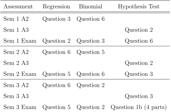
2.1 for an outline of the topics chosen and their appearance in the assessment items.
Table 2.1: Question mapping across semesters
Assessment Regression Binomial Hypothesis Test
Sem 1 A2 Question 3 Question 6
Sem 1 A3 Question 2
Sem 1 Exam Question 2 Question 3 Question 6
Sem 2 A2 Question 6 Question 5
Sem 2 A3 Question 2
Sem 2 Exam Question 5 Question 6 Question 3 Sem 3 A2 Question 6 Question 2
Sem 3 A3 Question 3
Sem 3 Exam Question 5 Question 2 Question 1b (4 parts)
2.2
Data Collection
Student demographic data, including information such as study mode, cit-izenship status, and degree and major of study, was downloaded from the OLS. The final demographic database only included those students who had remained enrolled for the entirety of the semester, which was acceptable as the scope of this project includes only students whose progress throughout the teaching period is trackable up to and including the final exam.
usefulness of learning analytics for educators and researchers, where the goal is to integrate assessment and OLS data. Minor errors in the assessment marks were corrected during collation (e.g. small errors in summing of marks across an assessment item by markers).
As the OLS generates an access log for each object or activity that can be accessed by students, the access logs of interest were those that would provide insight into student engagement with material relevant to the three topics of interest (Table 2.1); OLS objects which required interaction from both on-campus and external (online) students best suited this purpose. For example, student interactions with online lectures were not considered useful as on-campus students could access this content through class attendance rather than through the OLS. Tutorial solutions, in contrast, were accessible only within the OLS for all students, and students who accessed the solutions were likely to have been genuinely interacting with the tutorial questions and, subsequently, the topic content. For this reason, the tutorial solutions relevant to the three topics of interest were chosen as OLS objects of interest for this research. It was also decided that the example exams access logs would be used, as they indicate engagement with revision material close to the final examination. The OLS logs for the three chosen topics’ tutorial solutions and the example exams were downloaded for each semester separately.
2.3
Data Cleaning
Cleaning was not required for the demographic data prior to merging and analysis with the other datasets.
Prior to the commencement of analysis, all students with any missing assess-ment data were removed from the assessassess-ment database. This was necessary because no mapping of topic understanding across the semester could be per-formed for students who did not complete all assessment items. In addition, the methods of multivariate analysis used in this project require that cases with missing values for any variable need to be removed.
The downloading of OLS logs for Semesters 2 and 3 2016 was straightforward, however for the Semester 1 2016 OLS data, the downloaded files only included access records dated on or after 6 May 2016. The OLS had stored the access logs for the majority of OLS objects in two separate files: one with logs gener-ated prior to 6 May 2016; and another with logs genergener-ated on or after 6 May. This problem was specific to the Semester 1 2016 OLS. These two databases were merged in R prior to merging with other data types (i.e. demographic and assessment data).
2.4
Preparation of the Data for Analyses
The original demographic data listed each student’s degree and major, with over 40 unique degrees listed in each semester. Each of the degree programs studied by students were sorted into one of four categories (Degree Type):
Business, Commerce, Law and IT (BusComLawIT)
Psychology
Science
Other
These categories align with the general perspectives held by course examin-ers about the composition of the student cohort, and are coherent from the perspective of the university’s program structure. The programs that students were enrolled in differed for each semester, and so the R code used to assign one of the four categories to each student was changed for each semester. Programs listed under the “Other” category included Engineering, Education, Arts and Professional Development; none of these programs have a compulsory require-ment for students to complete the statistics course that is the focus of this project, unlike the programs in the other three Degree Type categories.
The assessment data contained scores achieved by students for each question. For example, if a student achieved 10 out of 18 on a question, this mark would be recorded as 10 in the database. These scores were converted into percentage achievement by dividing the score by the question total, to enable comparisons in achievement between questions for the same topic with different totals in different semesters.
Cutoff dates for the access logs were implemented for the overall semester, so that the OLS data contained only interactions that occurred during the teaching period. Any logs of accesses made prior to the first day of the teaching period and after the final exam date were removed from the database.
gen-erated within a few minutes of each other. It is unknown if there is a precise cause for this, however given the short time period within which they occur it is not reasonable to interpret these records as unique interactions by the student. To mitigate this complication, any access logs generated on a given day (regardless of how many) were condensed into one single access record of that OLS object by that student. These unique days were then tallied to give a count variable representing the number of times the object was accessed by each student during the semester. This count was then further summarised to a binary categorical variable, indicating whether or not students had accessed the content at any stage during the teaching period.
2.5
Summary Statistical Methods
Summary statistics were performed for each of the three semesters to provide an insight into the makeup of the student cohort for each semester. R code for each of the analyses run can be found in Appendix A.
The distributions of the relevant variables for students in each cohort were explored using contingency tables and bar charts. The demographic variables “Study Mode” and “Degree Type” and the frequency of access of OLS objects were of primary interest.
Boxplots were used to compare the assessment achievements of both on-campus and external (online) students across both assessment items (the assignment and the exam) in the three chosen topics. Another set of boxplots was created to investigate the differences in assessment achievement for the two levels of OLS access (never accessed, and accessed at least once).
deter-mine whether or not they were significantly different from zero. The Wilcoxon Signed-Ranks test was chosen as it is a non-parametric test for comparing matched samples, and therefore does not require the underlying populations of assignment and exam scores to be normally distributed.
2.6
Cluster Analysis
Cluster analysis was performed in order to identify the existence of any natu-rally occurring distinct subgroups in the data. Each semester’s database was analysed separately. Cluster analysis methods are based on distance measures where a single distance value is calculated between any two cases (students) based on the variation (or difference) between them across multiple variables of interest. Clusters of cases (students) are then formed on the basis of defin-ing cluster membership which minimises distances between data points within a cluster, while maximising the overall distances between clusters (Manly, 2005).
There are many forms of distance measures available. For this research the Gower distance was used to calculate the distance matrix (a matrix of the mul-tivariate distances between each pair of cases), as the Gower distance allows mixed data types to be used in the analysis. This distance method differ-entiates between categorical and continuous variables by applying a relevant distance method to each, and then combining the distances into one final value representing the aggregate distance between two cases (Kalisch, 2012).
To find the distance between two cases (two students) on a continuous variable, the following equation is used:
d(ijf) = |xif −xjf| Rf
,
xif and xjf are the scores for case i and case j on variable f, and Rf is the
range of possible scores for variable f. The difference between the scores for both cases is divided by the range of possible scores so that the distance value calculated is between 0 and 1 (Kalisch, 2012).
The equation for the calculation of the distance between two cases on a cate-gorical variable is given below:
d(ijf) =
1, if students are different on variable f 0, if students are the same on variable f
Once the distances between the two cases on each variable are calculated, these distance values are aggregated into the final Gower distance using the following equation:
d(i, j) = 1 p
p
X
f=1
d(ijf),
where d(i, j) is the aggregate distance between cases i and j, p is the total number of variables included in the analysis, andf is the index of summation. The sum of all distance values is divided by the total number of variables, again to ensure that the final distance metric lies between 0 and 1. The distance matrix is then constructed from these final distance values, d(i, j). For the creation of the final distance matrix, a linear combination of the distances using weightings for each variable can be calculated, however for this analysis it was decided that the weightings would not be changed from the default of equal weightings for all variables. The final distance matrix is of (n×(n−1)) size, wherenis the original number of cases (students) in the semester dataset (Kalisch, 2012).
in each cluster that may not exist as an actual case in the dataset. It is an iterative procedure where cluster medoids are randomly selected, and then the distance matrix calculated earlier is used to assign each data point to its clos-est medoid. The algorithm then calculates if any data points in each cluster would provide a lower average distance if they were to be designated as the medoid instead of the original. If any data points are identified as potentially better medoids, then the process repeats for these new medoids, until the best medoids are found (Spector, 2011).
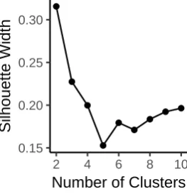
Partitioning around the medoids can be done only when the number of clusters to be generated is first defined. A metric known as silhouette width can be used to determine the level of appropriateness of the clusters that the data have been assigned to (Rousseeuw, 1987). For this cluster analysis, the PAM algorithm was run for many different numbers of clusters, and then the silhouette width values for each scenario were plotted to visually compare and determine the optimal number of clusters to be used. Silhouette width was used as it can be calculated with any distance metric, which is important since Gower distance calculation involves different distance metrics (Rousseeuw, 1987).
As described above, the cluster analysis performed in this research included both quantitative and categorical variables. The quantitative variables used were the achievement variables for the assignment and exam questions for the three chosen topics (six variables in total), while the categorical variables used included the demographic variables “Degree Type” (coded with levels ‘BusComLawIT’ (combined Business, Commerce, Law and IT factor), ‘Psy-chology’, ‘Science’ and ‘Other’) and “Study Mode” (coded with levels ‘Exter-nal’ and ‘On-campus’ for Semester 1 and 3, and coded with levels ‘Exter‘Exter-nal’, ‘On-campus Toowoomba’ and ‘On-campus Springfield’ for Semester 2) and the OLS access binary variables for the tutorial solutions for the three chosen topics (coded with levels ‘No Access’ and ‘At Least One Access’).
plot, which represents the relative distances between cases based on the dis-tance matrix. The scale of the axes of the ordination plot have no relationship with any of the original variables. The ordination plot provides a graphical representation of the approximate (relative) unitless distances between cases, to enable interpretation of how the clusters differ and the variance among cases within clusters. Care must be taken with interpretation, as the definition of clusters is a subjective process and may be influenced by the biases of the researcher.
The packages “dplyr” (Wickhamet al., 2017), “cluster” (Maechleret al., 2017) and “Rtsne” (Krijthe, 2015) were used to perform the cluster analysis in this project.
2.7
Principal Components Analysis
Principal components analysis (PCA) is a multivariate data reduction tech-nique that is based on the correlation between variables, rather than the dis-tance matrix used for cluster analysis. It identifies patterns of simultaneous variation by using either the correlation or the covariance matrix of the vari-ables, and constructs a new set of variables by using linear combinations of the original variables (Manly, 2005). These new variables, or principal compo-nents, are chosen so that the first accounts for as much variation in the data as possible, the second accounts for as much variation as possible that is not included in the first principal component, and so on until all variation in the data is accounted for.
co-efficients) of the original variables on the principal component (Manly, 2005). The composition of the principal component is given in the equation below (where Zi represents the ith principal component, Xj represents the jth
orig-inal variable and aij represents the loading of the jth original variable on the ith principal component):
Zi = p
X
j=1
aijXj
Because PCA is a data reduction technique, it is hoped in performing PCA that a relatively small number of principal components account for a large proportion of the total variation in the data. Interpretation of the principal components can be done via ordination plots, specifically bi-plots, which show a two-dimensional plot of the data with the first two principal components on the x- and y-axes, and vectors of the original variables superimposed to allow interpretation of their correlation with the principal components.
Basic PCA, in relying on the correlation (or covariance) matrix to calculate principal components, requires all variables to be continuous, as categorical variables do not correlate with other variables in a traditional sense. There are advanced PCA methods that allow the inclusion of categorical variables in the analysis, such as CATPCA (Linting & van der Kooij, 2012), however in this research the PCA was performed using only the continuous variables, and then the categorical variables were added to the model afterwards as supple-mentary variables. Their relationship with the principal components can be visualised, and interpreted descriptively, by adding their centroids to a bi-plot corresponding with the factor map of the continuous variables. The centroid of each category is based on the distribution of the cases in that category (Lˆe
et al., 2008).
Chapter 3
Results
Results from the analysis of Semester 3 2016 data are presented here in full as an exemplar. In addition, the results for Semester 1 and Semester 2 2016 are described in relation to corresponding Semester 3 2016 results, while the full set of results for these two semesters are presented in Appendices B and C. Semester 3 consisted of students enrolled externally, as well as on-campus at Springfield (there was no on-on-campus Toowoomba mode offered in this semester).
3.1
Assessment achievement
Difference in Assignment and Exam Achievement
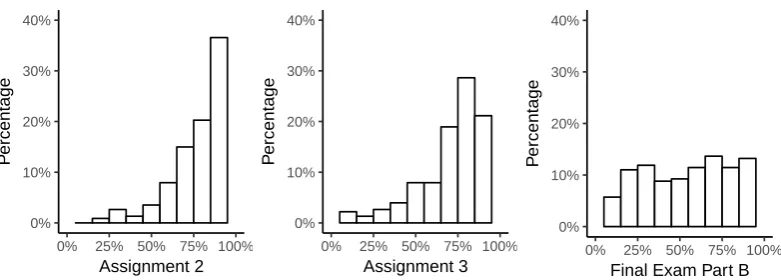
It is important to understand the general trends of achievement in the course to gain a better understanding of the cohort and the course. Figure 3.1 shows that achievement in the assignments is skewed to the left, with the majority of students achieving between 65% and 100%. On the final exam, however, the distribution is more even across achievement levels, indicating that there are more students performing poorly in the exam than in the assignments.
0% 10% 20% 30% 40%
0% 25% 50% 75% 100%
Assignment 2 P ercentage 0% 10% 20% 30% 40%
0% 25% 50% 75% 100%
Assignment 3 P ercentage 0% 10% 20% 30% 40%
0% 25% 50% 75% 100%
Final Exam Part B
P
ercentage
Figure 3.1: Distribution of overall achievement for each assessment item
the exam, Figure 3.2 shows differences in performance for each topic with his-tograms of the differences in achievement between each topic’s Assignment and Exam question (Difference = Exam −Assignment). Most students’ achieve-ment scores have decreased from the assignachieve-ment to the exam (the majority of the occurrences are negative). For all topics the tallest bin is between -10% and 10%, indicating that many students retain relatively consistent achievement in each topic across the two assessment items.
It must be noted that since the difference in achievement is calculated by tak-ing the assignment score away from the exam score, if a student has achieved perfect marks (100%) in the assignment, it is not possible for them to improve on this, and so they cannot get a positive difference between the assignment
0% 10% 20% 30% 40%
−100% −50% 0% 50% 100%
Regression P ercentage 0% 10% 20% 30% 40%
−100% −50% 0% 50% 100%
Binomial P ercentage 0% 10% 20% 30% 40%
−100% −50% 0% 50% 100%
Hypothesis Test
P
[image:42.595.106.497.94.234.2]ercentage
and the exam. However, if a student has achieved poor marks in the assign-ment, there is more opportunity to perform comparatively better on the exam. This may be contributing to the low frequencies of positive differences from the histograms. Similar trends to Semester 3 are displayed in Semesters 1 and 2 (refer to Figures B.2 and C.2 in Appendices B and C).
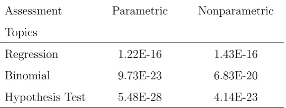
[image:43.595.156.445.638.747.2]To check whether there is a significant difference between the assignment and exam scores for each topic, t-tests were used. Table 3.1 gives the p-values of each test, both parametric (t-test) and non-parametric (Wilcoxon Signed-Ranks test). The differences between assignment and exam achievement are statistically significant for all topics. This, in conjunction with Figure 3.2, indicates that the performance on the invigilated exam is poorer in comparison to the assignments for a substantial number of students. These findings were reflected in the other semesters (refer to Tables B.1 and C.1).
Table 3.1: p-values for testing of differences between assignment and exam scores in the three topics
Assessment Topics
Parametric Nonparametric
Regression 1.22E-16 1.43E-16
Binomial 9.73E-23 6.83E-20
3.2
Relationships between data sources
Distribution of Demographic Data
The distribution of study mode by type of degree for the 227 students who were enrolled in the introductory statistics course in Semester 3 is presented in Table 3.2. Most noticeable is that the total number of external students enrolled (83%, n=188) is much greater than the total number of on-campus students (17%, n=39). The degrees studied by students are represented in four groups: the combined group of business, commerce, law and information technology (BusComLawIT) (43%, n=98), psychology (13%, n=29), science (27%, n=62) and other degrees (17%, n=38). For all Degree Types except BusComLawIT, the total on-campus enrolment count for each is under ten students, representing only 17% of the cohort in total. The combined Bus-ComLawIT degrees have the highest enrolment of all degree types, with 43% of total enrolment for Semester 3.
When compared with the frequency tables for the Semester 1 and Semester 2 cohorts (refer to Table B.2 and Table C.2 respectively), it can be seen that a smaller proportion of the Semester 3 cohort studied a degree in the BusCom-LawIT category than that of the other cohorts; in Semester 3, 43% of students studied under the BusComLawIT category, while in Semester 1 this category consisted of 58% of the cohort and in Semester 2 this category made up 63%
Table 3.2: Distribution of Degree Type by Study Mode
Degree Type External On-campus Springfield Total
BusComLawIT 77 21 98 (43%)
Psychology 22 7 29 (13%)
Science 58 4 62 (27%)
Other 31 7 38 (17%)
of the cohort. Conversely, the Other category made up 17% of the Semester 3 cohort, while only comprising 7% of the Semester 1 cohort and 5% of the Semester 2 cohort.
The proportion of external students was similar between Semester 3 (83%) and Semester 1 (78%). However, in Semester 2, this proportion changed substan-tially, with only 48% of students enrolled externally (the remainder divided between enrolling on-campus at Toowoomba (35%) or Springfield (16%)).
Access Records by Study Mode
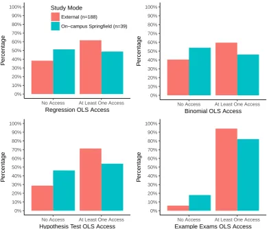
Learning analytics in this research context is dependent on the ability to track access to resources by students throughout the teaching period. Of particular interest is exploring the access habits of students in different demographic groups. The most relevant demographic variable available to access habits is study mode, as different study modes may be linked to different levels of engagement with the course. Figure 3.3 shows the distribution of access for each OLS object chosen for this project (tutorial solutions for each topic as well as example exams), with external and on-campus cohorts shown side-by-side for comparison.
0% 10% 20% 30% 40% 50% 60% 70% 80% 90% 100%
No Access At Least One Access
Regression OLS Access
P
ercentage
Study Mode
External (n=188)
On−campus Springfield (n=39)
0% 10% 20% 30% 40% 50% 60% 70% 80% 90% 100%
No Access At Least One Access
Binomial OLS Access
P ercentage 0% 10% 20% 30% 40% 50% 60% 70% 80% 90% 100%
No Access At Least One Access
Hypothesis Test OLS Access
P ercentage 0% 10% 20% 30% 40% 50% 60% 70% 80% 90% 100%
No Access At Least One Access
Example Exams OLS Access
P
[image:46.595.104.494.234.568.2]ercentage
When comparing these results with that of the Semester 1 and 2 cohorts, most of the results are similar, with a higher percentage of on-campus students hav-ing not accessed the resources than external students (refer to Figures B.3 and C.3). A notable difference between the on-campus Springfield cohorts of Semester 2 and Semester 3 is the higher proportion of students in Semester 2 who did not access the OLS objects. In particular, 44% of Semester 2 on-campus Springfield students did not access the example exams on the OLS, which is substantially higher than the 18% of on-campus Springfield students in Semester 3 and 12% of on-campus Toowoomba students in Semester 1 who did not access the example exams.
OLS Access by Demographic Data
It is important for course examiners to know the frequency at which their cohort is interacting with the learning material. Also of interest is the access habits of different subgroups within the cohort, to enable understanding of how students in differing circumstances may interpret the role of the OLS in supporting their learning.
Table 3.3 shows the percentage of students from each degree type who accessed each OLS object at least once throughout the semester. The example exams OLS object was the most frequently accessed OLS object for all degree types, with access being above 89% compared with access to all other objects of
Table 3.3: OLS access (percentage) for each degree type
OLS Objects BusComLawIT (n=98)
Psychology (n=29)
Science (n=62)
Other (n=38)
Regression 60 62 56 61
Binomial 64 52 48 58
Hypothesis Test 68 72 65 71
interest not being higher than 73%. Table 3.3 also indicates that the hypothesis test topic tutorial solutions were the most popular tutorial solutions across all degree types. Out of all the degree types, the students in the Science degree category tended to access the least frequently, with the lowest percentage access for all OLS objects except for the example exams.
When comparing these OLS access frequencies with those from Semesters 1 and 2 (see Tables B.3 and C.3), it can be seen that the only consistent trend is that the example exams are always accessed more frequently than the other OLS objects. Of interest is the stark difference between Semesters 2 and 3 in terms of the access to example exams. For Semester 3, the example exams access rates (regardless of Degree Type) were always above 89%, however for the Semester 2 cohort, the example exams access rates were consistently between 70% and 80%. This indicates a cohort-wide trend of reduced access to the example exams in Semester 2.
Note that Figure 3.3 and Table 3.3 are the only places where access to the example exams OLS object is presented – in all other parts of this project, only the access records for the tutorial solutions for the chosen topics are used.
Distribution of Assessment Data by Study Mode
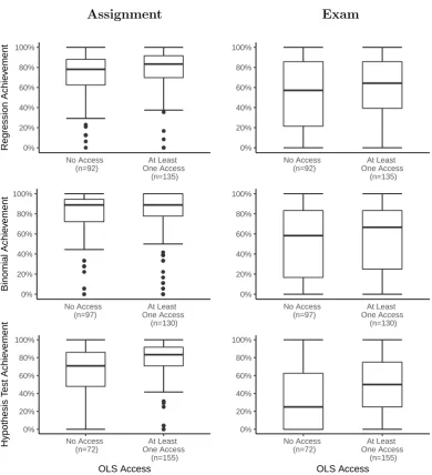
Also evident from Figure 3.4 is the considerably larger interquartile ranges of the exam question achievement scores when compared to the correspond-ing assignment questions, indicatcorrespond-ing that there is more spread in the exam results. Students (regardless of study mode) tend to perform relatively well on assignment questions (with the lower quartile of assignment achievement scores located at or above 60%). In the exam questions, however, students are more likely to perform at a lower standard on average, with the lower quartile often being located between 20% and 40%. The lower quartile of the hypoth-esis test exam question for on-campus students was located at 0%, indicating that this questions was most likely not attempted by many of the on-campus students.
The spread (measured by the interquartile range) of the binomial assignment achievement scores in Semester 1 is greater than that of the Semester 3 bi-nomial assignment achievement scores, for both on-campus and external stu-dents. In addition, achievement in the hypothesis test exam question by the Semester 1 cohort was generally much higher than that of the Semester 3 co-hort, again for all study modes. Apart from these differences, all other results are extremely similar between the two semesters (refer to Figure B.4).
Assignment Exam 0% 20% 40% 60% 80% 100% External (n=188) On−campus Springfield (n=39) Regression Achie v ement 0% 20% 40% 60% 80% 100% External (n=188) On−campus Springfield (n=39) 0% 20% 40% 60% 80% 100% External (n=188) On−campus Springfield (n=39) Binomial Achie v ement 0% 20% 40% 60% 80% 100% External (n=188) On−campus Springfield (n=39) 0% 20% 40% 60% 80% 100% External (n=188) On−campus Springfield (n=39) Study Mode Hypothesis T est Achie v ement 0% 20% 40% 60% 80% 100% External (n=188) On−campus Springfield (n=39) Study Mode
Distribution of Assessment Data by OLS access categories
Figure 3.5 shows similar plots to those in Figure 3.4, however the boxplots are categorised by the number of times the OLS object had been accessed, rather than study mode. The analysis of assessment and OLS data in combi-nation is a critical aim of the application of learning analytics in this research project.
In most of the plots in Figure 3.5, it can be seen that the students who did not access the OLS object at all performed, on average, slightly worse than those who accessed once or more. With the exception of the Binomial Assignment question, the median achievement of students who never accessed the relevant tutorial solutions is lower than that of students who accessed the tutorial solutions at least once.
Similar to Figure 3.4, the interquartile ranges of the exam achievement scores are larger than that of the assignment achievement scores, indicating higher variability in student achievement during the exam. There are many outliers in the lower end of achievement scores for the assignment questions regardless of frequency of OLS access. Also evident is that the difference in median achievement when comparing students who did not access to students who accessed at least once is much larger for the exam questions compared to the assignment questions. This indicates that accessing the OLS tutorial solutions at least once may lead to better performance on invigilated assessment at the end of the semester.
Assignment Exam 0% 20% 40% 60% 80% 100% No Access (n=92) At Least One Access (n=135) Regression Achie v ement 0% 20% 40% 60% 80% 100% No Access (n=92) At Least One Access (n=135) 0% 20% 40% 60% 80% 100% No Access (n=97) At Least One Access (n=130) Binomial Achie v ement 0% 20% 40% 60% 80% 100% No Access (n=97) At Least One Access (n=130) 0% 20% 40% 60% 80% 100% No Access (n=72) At Least One Access (n=155) OLS Access Hypothesis T est Achie v ement 0% 20% 40% 60% 80% 100% No Access (n=72) At Least One Access (n=155) OLS Access
3.3
Multivariate Analyses
Cluster Analysis
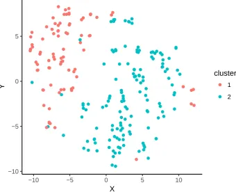
Figure 3.6 indicates that using two clusters provides the highest silhouette width, so two clusters were used in this analysis. The clusters can be visualised using the 2D ordination plot as shown in Figure 3.7. Although the two clusters neighbour each other closely with no gap in-between, they are still recognisable as separate clusters. There is some overlap of the clusters, with a few cases occurring well within the opposite cluster to which it was assigned. This may be due to variation of those cases from the other cases in the cluster on a couple of the original 6 continuous and 5 categorical variables included in the calculation of the distance matrix. There are very few cases that considerably overlap the cluster boundary compared with the total number of cases.
Within each cluster, the distances between cases in both dimensions are a rep-resentation of the average distances between cases among all variables. There-fore, the medoids for each cluster (the cases central to each cluster) will not be reported as they represent the average characteristic of the cluster only and do not provide perspective on the variation within each of the closely neigh-bouring clusters. It is more appropriate instead to use summary statistics of the clusters as measures of their overall characteristics.
0.15 0.20 0.25 0.30
2 4 6 8 10
Number of Clusters
[image:53.595.233.365.551.688.2]Silhouette Width
−10 −5 0 5
−10 −5 0 5 10
X
Y
cluster
1
[image:54.595.126.467.102.378.2]2
Figure 3.7: 2D ordination plot of aggregate distances between cases, with cases coloured by assigned cluster
Cluster Analysis – Summary Statistics on Clusters
(13.1%) between the two clusters.
Figure 3.8 displays the relationship between cluster membership and OLS ac-cess. It can be seen that the majority of students in Cluster 1 (around 85% for Regression, around 90% for Binomial and around 70% for Hypothesis Test) are students who never accessed the respective tutorial solutions, and that the majority of students in Cluster 2 (around 85% for Regression, around 85% for Binomial, and around 90% for Hypothesis Test) are students who accessed the respective tutorial solutions at least once.
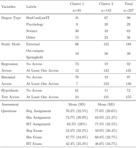
Table 3.4 also shows that there are noticeably more external students in Cluster 2 than in Cluster 1 (66 students in Cluster 1, 122 students in Cluster 2), further supporting the trend shown in Figure 3.3 that a greater proportion of external students access the OLS resources (since Cluster 2 is mostly comprised of students who accessed at least once, see Figure 3.8).
Table 3.4: Frequencies of Degree Type, Study Mode and OLS Access, and mean and standard deviation of achievement in assessment questions, by Clus-ter
Variables Labels Cluster 1
n=85
Cluster 2 n=142
Total n=227
Degree Type BusComLawIT 31 67 98
Psychology 9 20 29
Science 30 32 62
Other 15 23 38
Study Mode External 66 122 188
On-campus Springfield
19 20 39
Regression No Access 73 19 92
Access At Least One Access 12 123 135
Binomial No Access 78 19 97
Access At Least One Access 7 123 130
Hypothesis No Access 61 11 72
Test Access At Least One Access 24 131 155
Assessment Mean (SD) Mean (SD)
Questions Reg Assignment 70.2% (22.5%) 77.6% (20.6%) Bin Assignment 73.7% (29.9%) 82.9% (21.2%) HT Assignment 65.5% (28%) 77.3% (22.5%) Reg Exam 53.2% (32.2%) 59.9% (30.4%) Bin Exam 47.7% (34.8%) 60.8% (32.7%)
0% 10% 20% 30% 40% 50% 60% 70% 80% 90% 100%
No Access At Least One Access
Regression OLS Access
P
ercentage
Cluster 1 (n=85) Cluster 2 (n=142)
0% 10% 20% 30% 40% 50% 60% 70% 80% 90% 100%
No Access At Least One Access Binomial OLS Access P ercentage 0% 10% 20% 30% 40% 50% 60% 70% 80% 90% 100%
No Access At Least One Access
Hypothesis Test OLS Access
P
ercentage
Figure 3.8: OLS access by cluster membership
Principal Components Analysis
The individual and cumulative percentage variation explained by each princi-pal component are given in Table 3.5, and the loadings of each original variable on each principal component are given in Table 3.6. Table 3.5 shows that the first two principal components cumulatively explain 72% of the total variation in the data. The loadings given in Table 3.6 show that each of the original vari-ables are moderately weighted on the first principal component, while for the second principal component the assignment variables are weighted positively, and the exam variables are weighted negatively.
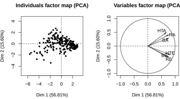
Visual representations of the first two principal components (both the individ-uals factor map and the variables factor map) are given in Figure 3.9. The individuals factor map (left plot) shows that the cohort had much greater spread with respect to the first principal component (the x-axis), especially
Table 3.5: Percentage variation explained by each principal component
Table 3.6: Loadings of the original variables on each principal component
PC1 PC2 PC3 PC4 PC5 PC6
Regression Assignment 0.41 0.30 0.65 -0.01 0.57 -0.02 Binomial Assignment 0.41 0.43 0.20 0.18 -0.75 -0.06 Hypothesis Test Assignment 0.37 0.51 -0.68 -0.22 0.25 0.17 Regression Exam 0.39 -0.42 0.11 -0.78 -0.19 0.13 Binomial Exam 0.42 -0.42 -0.09 0.52 0.04 0.61 Hypothesis Test Exam 0.44 -0.33 -0.24 0.22 0.10 -0.76
−6 −4 −2 0 2
−4
−2
0
2
4
Individuals factor map (PCA)
Dim 1 (56.81%)
Dim 2 (15.60%)
−1.0 −0.5 0.0 0.5 1.0
−1.0
−0.5
0.0
0.5
1.0
Variables factor map (PCA)
Dim 1 (56.81%)
Dim 2 (15.60%)
RA BA HTA
[image:58.595.103.476.430.635.2]RE BEHTE
for cases in the bottom left quadrant. There was also a reasonable amount of spread with respect to the second principal component, with students in the bottom left quadrant again displaying the most variation. The variables factor map (right plot) in Figure 3.9 visualises the variable loadings on the principal components from Table 3.6 and confirms that all continuous vari-ables are weighted in the same direction with respect to the first principal component; this principal component can therefore be interpreted as an “over-all achievement” component. The second principal component differentiates to some extent between achievement in the assignment and achievement in the exam. The vectors on the variables factor map, in conjunction with the indi-viduals factor map, indicates which variables were separating cases at different extremes of the map from the rest of the group.
Students on the left hand side of the x-axis (Figure 3.9) performed poorly overall in the assessment items, according to the first principal component. Extending the assignment vectors back into the bottom left quadrant, it can be seen that the students in this quadrant stand out from the group due to their underperformance in the assignment questions. Likewise, students who performed poorly in the exam questions are located in the top left quadrant. Comparing the top left quadrant to the bottom left quadrant, it can be seen that the majority of cases in the top left quadrant are closer to the centre of the cohort than those in the bottom left, indicating that it is more commonplace within the whole cohort to perform badly in the exam questions than in the assignment questions. It is also evident that many students in the bottom left quadrant are further to the left on the x-axis than students in the top left quadrant, highlighting that students who underperform on the assignment questions tend to perform worse in the course overall, with respect to the first principal component.
that the factor separating these students from the group is their outstanding performance on the exam questions. Students who performed well on the assignment questions (located in the top right quadrant) are very close to the centre of the group, which shows that high performance on the assignments is not only a common occurrence within the cohort, but also does not distinguish student performance from the cohort average compared to high achievement in the exam questions.
The weightings and loadings of principal components are extremely similar between Semester 3 and the other semesters, indicating that the principal components have identified robust trends in the data. Refer to Tables B.5, B.6, C.5 and C.6, as well as Figures B.9 and C.9 for the comparison. For example, across all three semesters the cumulative percentage of total variation explained by the first two principal components is between 70% and 74%, and the first two principal components have similar weightings (all the original variables are moderately weighted against the first principal component, and the assignment question variables are oppositely weighted against the second principal component when compared to the exam question variables). Across all three semesters, the combination of the individuals and the variables factor maps showed that low performance in the assignment made cases stand out considerably from the group. The only notable difference in the PCA for the three semesters is that the students in Semester 2 who performed badly on the exam questions were more separated from the rest of the group than in Semesters 1 and 3 (see Figures B.9 and C.9).
−0.5 0.0 0.5
−0.5
0.0
0.5
Individuals factor map (PCA)
Dim 1 (56.81%)
Dim 2 (15.60%)
BusComLawIT
Psychology
Science
Other External
On−campus Springfield
No Access
At Least One Access
No Access At Least One Access
No Access
At Least One Access
[image:61.595.104.478.238.573.2]Degree Type Study Mode Regression Access Binomial Access Hypothesis Test Access
students in the degree types ‘Science’ and ‘Other’ performed better than ‘Bus-ComLawIT’ and ‘Psychology’ students, and students who access the OLS re-sources performed better than students who do not. With respect to the second principal component, it can be seen that students in the ‘Other’ and ‘Science’ degree type categories performed well on exams compared to the other degree types.
The qualitative supplementary variables in both Semester 1 and 2 also show that students who do not access the OLS resources for each topic consistently performed worse with respect to the overall achievement principal component (PC1) than students who accessed them at least once. Students in the ‘Sci-ence’ degree type achieved highly on exams just as they did in Semester 3, however students in the ‘Other’ category varied in their performance (average in Semester 1 and poor in Semester 2).
Chapter 4
Discussion and Conclusions
This chapter discusses the major findings in the cohort identified by the sum-mary statistics, then discusses the results and utility of both the descriptive statistics and multivariate statistical models used in this project, and finally gives an overview of the potential interventions identified from, and limitations of, the conclusions drawn from the analyses. This will be expressed within the context of the service course analysed in this research, both from the point of view of the service course itself within the university, and where appropriate also from the perspective of a wider application of the techniques and method-ologies used in this project to other scenarios outside of the specific context of this research. The implications and limitations of the data collation process (including cleaning and merging of data) on data analytics in the education field will also be discussed, as these combined data are not generally readily available.
4.1
Trends and relationships in the data
There was a clear disparity between average student performance in the assign-ments and in the final exam (see Figures 3.1 and 3.2). The major functional differences between these two types of assessment is the time that they are due (assignments are due throughout the semester, while the final exam is at the end) and the restrictions imposed on access to materials and time (assign-ments impose no restriction, whereas the final exam poses both a restriction on reference materials and a time limit of two hours). It is plausible that these differences contributed to the overall differences in achievement. In the past, high levels of anxiety have been reported by students in regards to the invig-ilated examination, which may affect performance. In the final examination, although material is restricted, students are allowed to use a double-sided A4 sheet of their own notes to aid them, as well as statistical formulae and tables that are provided with the examination paper. The main restriction imposed by the exam, therefore, is that it is invigilated and limited by time. The anal-ysis of assessment data in combination with both demographic and OLS data enabled an insight into some other factors that may be influencing this differ-ence in achievement in the context of this particular undergraduate statistics course, which will be discussed further throughout this chapter.
on-campus enrolment.
The BusComLawIT degree type was the most popular category in all semesters. The most popular degrees at the university either do not require completion of this statistics course, or are degrees that fall under the BusComLawIT cat-egory, so this result was not unexpected as the proportion of students enrolled in a BusComLawIT program is likely to be higher than that of the other degree types.
The proportion of the cohort that did not access the tutorial solutions was above 25% for all topics across all three semesters and all study modes, which is substantial given that students cannot access these resources elsewhere (see Figure 3.3 and Table 3.3). It may be that students complete the tutorials and then do not bother to download the tutoria