Analysis of Packaging and Deployment of Ultralight Space Structures

(1)

ANALYSIS OF PACKAGING AND DEPLOYMENT

OF ULTRALIGHT SPACE STRUCTURES

Thesis by Lee Wilson

In Partial Fulfillment of the Requirements for the Degree of

Doctor of Philosophy

California Institute of Technology Pasadena, California

2017

(2)

c 2017 Lee Wilson

(3)

(4)

Acknowledgments

Out of all people who helped me get to this point, the most deserving of my thanks is my advisor, Professor Sergio Pellegrino, who has gone above and beyond in his support and advice. His hands on approach has kept me on track and focused on solving interesting research questions. His tireless support has helped me finally make it to the end of the PhD journey.

I am also grateful for my fellow graduate student and post-doc collaborators, including Christophe Leclerc, Manan Arya, Miguel Bessa, and James Umali, for enabling my research.

To the fellow members of the AAReST project, who I have spent hours discussing spacecraft design and testing with, thank you. In particular Dr. Federico Bosi for sharing the hours spent by the shake table, Dr. Nicolas Lee and Dr. Steve Bongiorno for being able to bounce microsatellite subsystem design ideas off, and Serena Ferraro for carrying on the design and testing of the sub-system I poured my heart and soul into. I am also grateful to Dr. Gregory Davis, John Baker, and Dr. James Breckinridge for advice and mentorship.

Of course I also want to thank the Caltech staff for helping me with the more hands on aspect of my research, in particular Petros Arakelian for help in the lab, and John van Deusen, Joe Haggerty, and Ali Kiani for advice in machining and design. Thanks also to Kate Jackson, Christine Ramirez, and Dimity Nelson who kept the administrative part of my work running smoothly.

And of course, I want to thank my fellow members of the Space Structures Laboratory, for ideas, discussion, and support, including but not limited to Dr. Melanie Delapierre, Dr. John Steeves, Dr. Kristina Hogstrom, Thibaud Talon, Dr. Keith Patterson, Dr. Ignacio Maqueda Jimenez, Dr. Xin Ning, Yuchen Wei, Maria Sakovsky, and Gina Olson.

(5)

Abstract

This thesis presents a new approach to modeling in finite element analysis (FEA) creased thin-film sheets such as those used for drag sails, as well as modeling the packaging behavior of coilable deployable booms. This is highly advantageous because these deployable space structures are challenging to test on the ground due to their lightweight nature and the effects of gravity and air resistance. Such structures are utilized in the space industry due to their low mass and ability to be packaged into a small volume during their launch into space.

It is shown that removing the crease bending stiffness in creased sheets still allows the deploy-ment behavior of a benchmark problem to be captured, including deploydeploy-ment forces and equilibrium configurations. In addition, folding creased sheets from a flat state into a packaged configuration can result in crease crumpling and excessive wrinkling. To avoid this the Momentless Crease Force Folding (MCFF) technique is developed.

Further presented is the behavior of tape springs and Tubular Rollable and Coilable (TRAC) booms when coiled to radii greater than their natural bend radius. Under these conditions the booms can form multiple localized folds which may jam during boom deployment. Understanding this behavior is important for extending the use of these booms to large scale space structures such as orbital solar power stations.

A useful analytical model is developed determining when the localized folds in a tape spring will bifurcate and is verified against simulation results. Additionally, a numerical model of the wrapping an isotropic tape spring around a hub with a radius greater than the localized fold radii is validated against physical experiments. This model is used to predict trends in the force required to fully wrap a tape spring around a given hub radii.

(6)

Published Content and Contributions

[1] Conte, D., Budzyn, D., Burgoyne, H., Di Carlo, M., Fries, D., Grulich, M., Heizmann, S., Jethani, H., Lapˆotre, M., Roos, T., Serrano Castillo, E., Scher-rmann, M., Vieceli, R., Wilson, L., Wynard, C.Innovative Mars Global International Exploration (IMaGInE) Mission-First Place Winning Paper. InAIAA SPACE 2016 (2016), p. 5596. DOI: http://dx.doi.org/10.2514/6.2016-5596

L.W. researched and authored the in-situ resource utilization, space solar power and lander mass estimate sections of the paper.

[2] Leclerc, C., Wilson, L., and Pellegrino, S. Characterization of ultra-thin composite triangular rollable and collapsible booms. In 4th AIAA Spacecraft Structures Conference, (2017), p. 0172. DOI: http://dx.doi.org/10.2514/6.2017-0172

L.W. performed experiments and numerical analysis on the coiling of ultra-thin composite booms and co-authored the paper.

[3] Ota, N., Wilson, L., Neto, A. G., Pellegrino, S., and Pimenta, P. Nonlinear dy-namic analysis of creased shells. Finite Elements in Analysis and Design 121 (2016), 64-74. DOI: https://doi.org/10.1016/j.finel.2016.07.008

L.W. performed numerical analysis on the snapping behavior of hemispherical polymer shells and co-authored the numerical examples section of the paper.

[4] Umali, J. A., Wilson, L., and Pellegrino, S.Vibration response of ultralight wrapped spacecraft structures. In4th AIAA Spacecraft Structures Conference (2017), p. 1115. DOI: http://dx.doi.org/10.2514/6.2017-1115

(7)

[5] Wilson, L., Pellegrino, S., and Danner, R. Origami sunshield concepts for space telescopes. In 54th AIAA/ASME/ASCE/AHS/ASC Structures, Structural Dynamics, and Materials Conference (2013), p. 1594. DOI: http://dx.doi.org/10.2514/6.2013-1594

(8)

List of Figures

2.1 Artist impressions of deployed solar sails for (a) IKAROS [43], and (b) LightSail-1 [6]. 6

2.2 Cylindrical carbon fiber boom incorporating dog-bone cutout hinges in (a) deployed

configuration, and (b) folded configuration. . . 7

2.3 Tape spring [51] . . . 8

2.4 Exploded hub view of a CubeSat boom in initial stage of deployment [16]. . . 8

2.5 Storable Tubular Extendible Member booms [42] (a) Pure STEM (b) bi-STEM (c)

Interlocking bi-STEM. . . 9

2.6 Example of a carbon fiber Collapsible Tubular Masts developed by DLR [7]. . . 9

2.7 Schematic of a TRAC Boom [4]. . . 10

2.8 Abaqus simulation of a systematically creased sheet with a Miura-Ori crease pattern

[40]. . . 13

2.9 (a) Infinitesimal element of a thin-shell laminate with force and moment resultants,

and (b) Infinitesimal element of a thin-shell laminate including coordinate notation

for individual plies [9]. . . 14

2.10 Moment-angle relationship for a general tape spring [45]. . . 18

2.11 Tape spring bending in (a) opposite-sense, and (b) equal-sense [45]. . . 19

2.12 Schematic of a tape spring with a localized fold distanceyaway from a clamped end [45]. 20

2.13 Deployment sequence of a 0.54 m long tape spring with a localized fold of 90o in the

middle. Time delay between successive frames is 0.04 s [45]. . . 21

2.14 The solid lines are the predictions ofθandλduring deployment, based on an impulse-momentum formulation [45]. The circles and crosses correspond to experiment

mea-surements of θ andλ, respectively. . . 21

(14)

2.16 Deployment plot of a coiled tape spring under opposite sense bending on a fixed spool.

Crosses are experimental results; solid lines are analytical predictions. Top solid line

is the deployment assuming no air drag, lower solid line includes air drag with a tuned

drag coefficient [45]. . . 24

2.17 Folding stages of a composite tape spring hinge in Abaqus/Explicit [26] (a) Initial

configuration, (b) Rigid plates compress tape springs, (c) Boundary conditions fold

hinge. . . 24

2.18 Coiled composite tape spring in Abaqus/Explicit [47]. Contours correspond a failure

index. . . 25

2.19 TRAC boom cross-section including variable names [34].. . . 26

2.20 TRAC boom buckling mode [4]. . . 26

2.21 FEA image of ‘triangular buckles’ identified in TRAC booms when coiled to a radius

greater than its natural bending radius [34] (a) close up of ‘buckle’, and (b) a series

of ‘buckles’. . . 27

3.1 Schematics of a crease cross-section, meshed with thin-shell elements of length L. (a) Initial configuration and (b) configuration with bending moment M applied . . . 30

3.2 (a) Vertex not subjected to tie constraint in LS-Dyna due to insufficient overlap

be-tween the three slave parts and the master part. (b) Close up of vertex V1,1 after

surface has been meshed in LS-Dyna. Black dots are nodes from facetsF2,1, F2,2, and

F1,3 that have their translational degrees of freedom tied to facet F1,2. Green

high-lighted regions are included in the self-contact condition, white regions are excluded

to avoid interference with the creases. . . 32

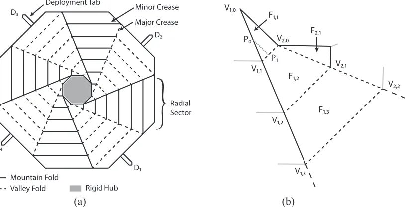
3.3 (a) Test case GP92 crease pattern that enables wrapping a thin-film around a

polyg-onal hub. Here there n= 8 major creases and m= 6 minor creases per radial sector. This corresponds to six quadrilateral and one triangular facets per radial sector. (b)

First three facets in radial sector 1, facets are labeledFi,j and verticesVi,j. . . 33

3.4 Average radial force required to deploy the folded GP92 creased film [3].. . . 34

3.5 Top views of experiment at force equilibrium points. Snapshots taken at df = 0.24,

(15)

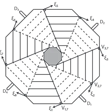
3.6 GP92 fold pattern showing local coordinate directions ξi, associated with vertices

Vi,7. To enforce symmetry these vertices are constrained to not move inξi directions

during folding. During the deployment stage radial displacement boundary conditions

are applied to D1−D4. . . 35

3.7 (a) Abaqus/Explicit FEA model of GP92 crease pattern with n = 8, m = 6. (a) Isometric view, and (b) top view. Yellow triangles correspond to connector elements

that model the creases. . . 36

3.8 (a) Schematic of rotational boundary conditions applied to the triangular facets during

step 1. . . 38

3.9 Von Mises stresses within the creased thin-film sheet during folding in Abaqus/Explicit.

(a), (c) the end of the rest period after folding, and (b), (d) 0.07 s through the

wrap-ping step, corresponding to hub rotation of 80◦. . . 39

3.10 Energy in Abaqus/Explict wrapping simulation of the GP92 crease pattern. . . 40

3.11 Removing elements closest to the hub vertices, to reduce the stress concentration. . . 40

3.12 Von Mises stresses within the creased thin-film sheet during folding for the Abaqus/Explicit

scenario where the vertices closest to the hub were removed. (a), (c) the end of the

rest period after folding, and (b), (d) 0.14 s through the wrapping step, respectively. . 41

3.13 Energy in Abaqus/Explict simulation of GP92 crease pattern for the case where

ele-ments surrounding the vertices closest to the hub have been removed. . . 42

3.14 Minor crease between the triangular facet and an adjacent quadrilateral facet (a) end

of wrapping step, and (b) first increment into the following rest step. Other facets are

hidden for clarity. . . 42

3.15 LS-Dyna FEA model of GP92 crease pattern. . . 43

3.16 Self-contact surface implemented for the LS-Dyna simulation of GP92 crease pattern.

Self-contact surface not defined for the elements along one side of each crease to avoid

conflict between crease tie-constraint and self contact. . . 44

3.17 Schematic of a creased surface being folded by point, line and pressure loads. . . 46

3.18 (a) Von Mises stress distribution in the wrapped sheet 75% of the way through folding.

Stress concentrations up to 141 MPa are present at the vertices of the triangular facets.

(16)

3.19 Close up of the triangular facet crumpling during folding at (a) 23% and (b) 30%

of the way through the folding step. To clearly show the crease line between the

triangular and quadrilateral facets the individual facets are shown in separate colors,

and the hub hidden for clarity. . . 47

3.20 Internal and kinetic energy in final LS-Dyna packaging simulation. Packaging ends at

0.016 s, and viscous damping is applied for 0.016 s following that. . . 48

3.21 Von Mises stress distribution at end of wrapping stage for LS-Dyna simulation

incor-porating pressure, line and point loads (a) Isometric view, and (b) top view. . . 49

3.22 The minimum principle in-plane stress for the initially flat simulation, with close up

views of the inner rings of triangular and quadrilateral facets when (a) 20% folded

and (b) fully folded. The hub is not shown for clarity, and the viewing angle is the

same in both (a) and (b). . . 50

3.23 MCFF algorithmic approach to model the folding of creased sheets in LS-Dyna. . . . 51

3.24 Top view of a single GP92 major creaseline when starting in an initially folded

con-figuration. Vertices Vi,j+1 are a radial distance w further out from Vi,j because of

non-zero θ0.. . . 53

3.25 Cross-section of crease. Minimum initial fold angleθ0is constrained by Equation 3.8 so

nodes adjacent to creases do not start the simulation with initial contact interference.

In a simulation moment M depends on initial crease angle θ0 and crease stiffness k(θ). 53

3.26 LS-Dyna model of the GP92 crease pattern when starting from an initially folded

configuration. (a) Isometric view, and (b) top view. . . 54

3.27 Tab displacement (df) during deployment and the corresponding mass nodal damping

(β) used to remove excess kinetic energy. . . 55

3.28 Deployment force results from LS-Dyna mesh convergence study. n corresponds to the number of elements along the edge of every the triangular facet. . . 56

3.29 Comparing LS-Dyna deployment force profiles for BWC and C0 shell elements for (a) the initially folded case and (b) packaged via MCFF technique, and comparing

Abaqus/Explicit deployment force profiles for S3 shell elements for the initially folded

(17)

3.30 Top and isometric views of the initially folded LS-Dyna simulation at equilibrium

configurations corresponding to df = 0.23, 0.42, 0.62 and 0.80. . . 58

3.31 Smoothed radial force data (left) required to deploy crease pattern and the

corre-sponding energy (right). (a), (b) are LS-Dyna results when starting from an initially

folded configuration. (c), (d) show Abaqus results starting from an initially folded

configuration. (e), (f) are LS-Dyna results when first folding from a flat state. . . 60

4.1 Schematic of a clamped tape spring with a single localized fold.. . . 63

4.2 Regions of the tape spring to which boundary conditions are applied during the folding

process. . . 65

4.3 Schematic of the folding process. The tape spring is first flattened in the middle, then

contact applied between the tape spring and the two cylinders of radius Rhub. Point

P is displaced, wrapping the tape spring through angleθ around a cylinder.. . . 65

4.4 Time derivative profile ofθ applied to give a smooth folding process. The area under the curve corresponds to θ= π₂ radians. . . 67

4.5 Isometric view of the folding process (a) Flattening tape spring, (b) Adding contact

with folding cylinders to form localized fold, (c) Final folded configuration. . . 68

4.6 Snapshots during unfolding for a tape spring meshed with Belytschko-Tsay

quadrilat-eral shell elements. The red and blue arrows correspond to the direction the tip and

localized fold are moving at time of snapshot. . . 68

4.7 Snapshots during tape spring deployment for a tape spring meshed withC0triangular shell elements. The red and blue arrows correspond to the direction the tip and

localized fold are moving, respectively, at the time of the snapshot. . . 69

4.8 λ and θ results from simulation using (a) quadrilateral Belytschko-Tsay shells, (b) quadrilateral S/R Hughes-Liu shells, (c) C0 triangular shell elements, and (d) fully integrated quadrilateral shell elements (Type -16). The black crosses and circles are

the experimental data points and the solid black lines are from the analytical model. . 70

(18)

4.10 The tape spring configuration immediately after the localized fold has reflected off

the base for tape springs meshed with (a) C0 triangular shell elements , and (b) fully integrated quadrilateral shell elements (Type -16). A close up of the region where the

tape spring has buckled when meshed with quadrilateral shell elements is also shown. 72

4.11 (a) Non-reflecting boundary conditions applied to bottom surface only. (b)

Non-reflecting boundary conditions applied to bottom surface, and sides of the solid element

layer nearest the tape spring. . . 73

4.12 λandθ results from implementing non-reflective boundary conditions for simulations using (a) C0 triangular shell elements, and (b) fully integrated quadrilateral shell elements, (Type -16). RB1 and RB2 correspond to setups in Figure 4.11(a) and 4.11(b). 74

4.13 Viscous pressure of 0.75 s−1 applied to tape spring surface during deployment to capture energy absorption. λ and θ results from simulation using (a) C0 _triangular

shell elements, and (b) fully integrated quadrilateral shell elements (Type -16). The

black crosses and circles are the experimental data points and the solid black lines are

from the analytical model. . . 75

4.14 Isometric views of (a) tape spring, including node sets and regions where boundary

conditions are applied, and (b) the central hub. After flattening, the axis of rotation

nodes are coincident to the green hub axis. The tape spring slots between the blue

cylinders and the whole hub is rotated so that it wraps around the green arcs. . . 76

4.15 Key stages in the coiling simulation. (a) Initial configuration, (b) Tape spring flattened

& contact with cylinders applied, (c) spool and cylinders rotated 28.4 radians, contact

between tape spring and spool applied, and (d) end of coiling simulation. . . 77

4.16 Energy density in the tape spring at the start of the uncoiling simulation. . . 79

4.17 Snapshots of the uncoiling of tape spring wrapped in opposite sense, meshed with

fully integrated LS-Dyna (Type -16), quadrilateral shell elements from around a fixed

spool. tcorresponds to the time from the start of deployment. . . 80

4.18 Comparison of the analytical model and the numerical model, utilizing fully integrated

quadrilateral shell elements when deploying from an (a) equal-sense, and (b)

(19)

5.1 Schematic of a tape spring folded around a cylindrical hub of radius Rh. (a) Initial

configuration, including localized bend radius of Ri. When displacementdapplied to

tape spring end, either (b) the localized bend radius increases or (c) the localized fold

bifurcates into two folds. . . 84

5.2 (a) Case 1 and 2 superimposed for γ = π₂ at d=dmax, where the straight, flattened

region is in contact with the hub. (b) The energy present in a tape spring at dmax

and γ = π₂ for case 1 and 2. . . 85

5.3 Piece-wise curvilinear cross-section of tape spring. . . 86

5.4 Experimental setup for wrapping a tape spring around a hub of radiusRhub= 4.125Ri. 88

5.5 (a) Schematic of experimental setup for measuring the coefficient of friction between

the hub and the tape spring. (b) Kinetic friction coefficients (µ) obtained from nine experimental runs. . . 89

5.6 Force profile corresponding to the opposite-sense wrapping of a steel tape spring

around a steel hub, where Rhub = 4.125Ri. Average of three repeated experiments. . . 90

5.7 Snapshots of the wrapping experiment, corresponding to the forces in Figure 5.6. (a)

Initial configuration and (b) immediately before bifurcation to three localized folds.

Left localized fold has increased in radius. (c) Immediately after bifurcation to three

localized folds, (d) four localized folds, (e) five localized folds, and (f) Six localized

folds. . . 91

5.8 (a) Initial configuration of coiling numerical simulation. (b) Tape spring folded with

two localized bends and temporary cylinders removed. Displacement dend applied to

fully coil tape spring. . . 92

5.9 (a) Initial configuration, (b) 0.04 s tape spring edges are compress and contact with

temporary cylinders enabled, (c) 0.17 s tape spring ends displaced so boom wraps

around cylindrical crushers, (d) 0.21 s contact with temporary cylinders removed,

and tape spring equilibrium configuration found. . . 94

5.10 Comparison of simulation tension force results during wrapping for tape springs meshed

with elements with side lengths = 3 mm, 2.5 mm, 2 mm, and 1.5 mm (dend = d).

(20)

5.11 Comparison of experimental results and simulation results with mass nodal damping

set to β = 1 s−1 and β = 10 s−1 for the entire wrapping simulation (dend =d). The

data has been smoothed with a 5 point moving average to remove noise. . . 95

5.12 Boom configurations in (a) initial configuration, (b) 14.2 mm displacement causes

bottom bend to increase in radius, (c) at 27.3 mm displacement bottom bend starts

to bifurcate in two, and (d) bottom bend has bifurcated at 27.5 mm displacement,

giving three localized bends. . . 97

5.13 The bending energy per unit length along the booms corresponding to the boom

configurations in Figures 5.12 (a) to (d). Length = 0 corresponds to the clamped end,

and the total length of the boom is 420 mm. . . 98

5.14 Boom configurations for the higher fidelity wrapping model in (a) four bends, (b) five

bends, (c) six barely visible localized bends, and (d) at d = 62.6 mm displacement three bends have flattened and conform to the hub radius, leaving three remaining

bends. . . 99

5.15 Force profile obtained from the high fidelity model.. . . 100

5.16 Energy components in the wrapping simulation after folding. (a) All energy, (b) close

up of internal energy, drops correspond to bifurcations, and (c) close up of kinetic

energy, where sudden build ups correspond to bifurcations. . . 101

5.17 Tape spring at the end of the wrapping simulation (a) Top view. (b) Close up of

sec-ondary fold. (c) Normal distance between the hub and tape spring. (d) Longitudinal

curvature of tape spring centerline in fully wrapped configuration. . . 103

5.18 Simulation setup for Rhub_Ri <1. . . 103

5.19 (a) Tension force required to fully wrap the steel tape spring for 0.4Ri< Rhub<0.65Ri

and 2.5Ri< Rhub<5.25Ri. (b) Close up of 0.35Ri< Rhub< Ri region. . . 105

5.20 Schematic of coiling simulation for Rhub< Ri. . . 106

5.21 (a) Point cloud of a carbon fiber tape spring specimen, generated from a FARO arm

laser scanner. (b) Center and radius of the tape spring cross-section along the boom

(21)

5.22 Ultra-thin carbon fiber tape spring configurations during wrapping. (a) Initial

config-uration, (b) fold radii increases, (c) configuration just before fold bifurcation, (d) fold

bifurcates into two, (e) four-fold configuration, and (f) fully wrapped configuration. . 108

5.23 Force profiles corresponding to opposite-sense wrapping experiments of an ultra-thin

carbon fiber tape spring around a steel hub.. . . 109

5.24 Comparison of force profiles required to tension an ultra-thin carbon fiber boom

around a hub of Rhub = 3.3Ri for (a) boom simulated with a constant cross-section,

and (b) boom simulated with cross-section varying along length to better match

phys-ical model. . . 110

6.1 (a) Initial configuration of coiling numerical simulation. (b) boom folded with two

localized bends and temporary cylinders removed. Displacementdend applied to fully

coil boom.. . . 115

6.2 Simulation results for a carbon-fibre TRAC longeron with constant cross-section and

bond region thickness of 0.142 mm. . . 116

6.3 Localized fold configurations that develop during the coiling of boom with uniform

cross-section and bond region thickness of 0.142 mm. (a) Initial two-fold configuration,

(b) configuration just before bottom fold bifurcates, (c) configuration when the bottom

fold has bifurcated into two, (d) configuration after bifurcation to five folds, (e) flanges

start to flatten instead of the localized folds bifurcating and, (f) fully coiled configuration117

6.4 Left: Initial TRAC boom experimental folded configurations. The left end of the

boom is rigidly mounted to the cylindrical hub, and the right end to an Instron tensile

testing machine. Right: Corresponding force profiles obtained during coiling. . . 119

6.5 Physical dimensions of the actual boom tested. (a) Height of bond region from a

reference surface when boom is resting on its flanges. Note that the flanges are only

in contact with the reference surface at Length = 0 and 535 mm. (b) Thickness of

bond region along the boom length. . . 120

6.6 Comparison of experimental results with (a) nominal simulation with no imperfections

(22)

6.7 Localized fold configurations that develop during coiling of boom with constant

cross-section and bond region thickness of 0.195 mm. (a) Initial folded configuration, (b)

the two localized folds have increased in radii, and (c) inner flange is in contact with

the hub in multiple locations. . . 122

6.8 (a) Close up of the localized fold closest to the clamped end in the initial folded

configuration, corresponding to Figure 6.7(a). (b) Curvature of inner flange edge,

outer flange edge and bond region centerline in the localized fold. Fold ends at length

= 130 mm. . . 123

6.9 (a) Initial configuration of coiling simulation. (b) Boom folded with single localized

bends and temporary cylinders removed. (c) Tension force Fmax is applied, tightly

wrapping boom about 90o arc of the hub. (d) Hub and pinned end rotated about hub

axis, coiling boom. . . 124

6.10 (a) Schematic of coiled boom, (b) Force vs tips deflection for unloading curve when

controllingγ and varying free lengthLF. (c) and (d) Boom configurations atF = 0.1

N for LF = 95 mm and 275 mm respectively. . . 126

6.11 Unloading and loading force vs tip displacement when free length is fixed at FL= 95

mm. . . 127

6.12 Top views of a boom wrapped to γ = 225o and initial free length of LF = 95 mm,

during re-loading of the boom after tension force has reached zero. Tension force is

(a) 0 N, (b) 0.3 N, and (c) 0.444 N. . . 127

A.1 (a) Test case GP92 crease pattern that enables wrapping a thin-film around a

polyg-onal hub. Here there n= 8 major creases and m= 6 minor creases per radial sector. This corresponds to six quadrilateral and one triangular facets per radial sector. (b)

First three facets in radial sector 1, facets are labeledFi,j and verticesVi,j. . . 139

A.2 GP92 fold pattern showing local coordinate directions ξi, associated with vertices

Vi,7. To enforce symmetry these vertices are constrained to not move inξi directions

during folding. During the deployment stage radial displacement boundary conditions

are applied to D1−D4. . . 139

A.3 Profiles of (a) line loads, (b) pressure loads and (c) point loads required to produce

(23)

A.4 Viscous damping profile applied after wrapping to remove kinetic energy and find an

equilibrium rest state . . . 140

B.1 (a) Initial setup of the tape spring wrapping simulations in Section 5.3. (b) Associated

dimensions and node sets. . . 143

B.2 Comparison of experimental results and simulation results with mass nodal damping

set to (a)β = 0.1−1 s−1 _{and (b)}_β _{= 10−1000 s}−1_{for the entire wrapping simulation.}

The data has been smoothed with a 5 point moving average to remove noise. . . 144

B.3 Wrapping simulation tension force results when the static and kinetic friction

coeffi-cients (µ) are varied, plotted against the observed experimental result. . . 145

B.4 Comparison of experimental results and simulation results with mass nodal damping

set toβ = 0−1 s−1 for the entire wrapping simulation. The data has been smoothed with a 5 point moving average to remove noise. . . 146

C.1 (a) Initial setup of the TRAC boom wrapping and coiling simulations in Sections 6.1.3

and 6.2. (b), (c) Associated dimensions and node sets. . . 148

(24)

List of Tables

4.1 Properties of tape springs tested by Seffen & Pellegrino [45], * indicates values derived

from bending moment experiments. . . 63

4.2 Boundary conditions applied to the tape spring to obtain the folded configuration.

f1(t), f2(t), g1(t), g2(t) were calculated from Equation 4.2. . . 66

4.3 Properties of tape spring tested in uncoiling experiments [45], * indicates values

de-rived from bending moment experiments. . . 75

4.4 Boundary conditions applied to the tape spring to obtain a coiled configuration. . . . 78

5.1 Summary of simulation steps for wrapping an isotropic tape spring around a hub,

where Rhub > Ri.. . . 93

A.1 Regions corresponding to Figure 3.3. To generate the hill and valley folds, for i = even forces are downwards (-z), for i= odd, forces are upwards (+z). . . 138

B.1 Boundary conditions for the simulation in Section 5.3. f1(t), f2(t), g1(t), g2(t) were

calculated with Equation 4.2 . . . 142

C.1 Boundary conditions for the simulation in Section 6.1.3. f1(t), f2(t), g1(t), g2(t) were

calculated from Equation 4.2 . . . 149

C.2 Boundary conditions for the simulation in Section 6.2. f1(t), f2(t), g1(t), g2(t) were

(25)

Chapter 1

Introduction

1.1

Overview

1.1.1 Deployable Structures

Deployable structures are an integral component of many spacecraft. One common feature of these systems is an ability to be tightly packaged during launch, and then deployed into a much larger configuration once in space. Deployable structures are implemented in applications as diverse as antennae, solar sails, solar panels, booms, and inflatable habitats. Of key importance is the pack-aging efficiency, stiffness in deployed configuration, and predictability of the deployment process. The predictability of deployment is often the most difficult to capture without flight testing.

1.1.2 Testing of Deployable Structures

(26)

Midway between testing on the ground and testing in space lie drop towers and zero-gravity flights. With drop towers the device to be tested is released from the top of a tower, and experiences weightlessness as it falls [39]. The effects of atmospheric drag can be reduced by pumping the air out, although there is always residual air resistance [22]. This approach is acceptable for small devices whose deployment time is on the order of seconds, that are either rugged enough to survive the fall or inexpensive enough to replace after each test.

For larger systems, on the order of meters, or those with longer deployment times, reduced-gravity flights are an option. Here an airplane flies in a series of parabolic arcs that allows the interior to experience weightlessness for durations of approximately 30 seconds. However, air-resistance is still present which can be problematic for deploying thin-film structures, such as solar sails.

In addition to these drawbacks, ground testing can be very expensive. An alternative to pure testing is to build either a numerical or analytical model of the deployment structure and use testing to validate this model. Once the model is validated, gravity and air-resistance can be removed from the model and the in-space performance estimated.

1.1.3 Analytical and Numerical Models of Deployable Structures

Many deployable structures utilize membrane or thin-shell components. There are two broad classes of approaches to modeling the behavior of these components. The first is a purely analytical approach. This can include capturing the bending energy within a coiled boom [8], or the stiffness in a series of folds in a packaged membrane [21].

However, these analytical approaches run into trouble when contact is a significant factor. Since the entire purpose of a deployable structure is to be packaged into a small volume, the effect of contact quickly becomes vitally important to include in the modeling approaches.

(27)

example is a creased thin-film sheet for a solar sail which has multiple overlapping layers when packaged. For these reasons, this work focuses on using explicit finite element analysis to capture both the static and dynamic behavior of ultralight deployable structures.

1.2

Objective and Scope

This work focuses on the deployment of creased thin-film structures, as well as strain-energy de-ployed tape springs and Triangular, Rollable and Coilable (TRAC) booms.

The deployment of creased thin-film structures differs significantly from traditional deployment mechanisms such as pantographs. Firstly, sheets with thicknesses on the order of tens of microns are extremely flexible and yet sufficiently stiff that it is important to consider the effect of bending stiffness in a numerical model. Secondly, the creases that are introduced can have a significant effect on both the deployment force and dynamic deployment behavior. One objective of this work is to determine if accurate quantitative and qualitative deployment forces can be obtained if the crease stiffness is removed entirely. Following this is the objective to develop a method for folding from flat and then deploying creased thin films structures in finite element software.

(28)

1.3

Layout of Dissertation

This dissertation consists of seven chapters, including this first introductory chapter.

Chapter 2 is a literature review of both creased thin-film deployable structures and strain energy deployed booms. The modeling techniques used to capture these structures’ behavior is then reviewed in detail.

Chapter 3 utilizes Abaqus/Explicit and LS-Dyna to capture the deployment behavior of wrapped polyimide sheets. These sheets are folded according to the GP92 fold pattern developed by Pelle-grino & Guest [45] and are potentially useful in solar-sail packaging schemes.

Chapter 4 compares experiments, analytical, and simulation models of tape springs to validate the simulation approach for strain-energy deployed booms. These simulations capture the dynamic behavior of unfolding a single tape spring hinge and the dynamic uncoiling of a tape spring from around a fixed spool.

Chapter 5 extends the body work on tape springs to the force profile required to coil them around hubs of radii greater than and less than their natural bend radius.

Chapter 6 presents the results of extending the simulations to TRAC booms manufactured from ultra-thin carbon fiber composite.

(29)

Chapter 2

Background

This thesis is primarily concerned with applying explicit finite element solvers to better understand and predict the deployment of ultralight deployable structures. In particular, the focus is on (a) creased thin-film sheets used for large planar spacecraft, such as solar sails and drag sails, and (b) strain-energy deployed booms such as tape springs and TRAC booms.

This chapter is split into three sections. The first section provides a general overview of the importance to space applications of these two classes of deployable structures. The second section focuses on modeling techniques currently used to analyze the behavior of large planar thin-film structures. The final section details the methods used to characterize and predict the behavior of strain-energy deployed booms.

2.1

Spacecraft Deployable Structures

Deployable structures are commonly used on spacecraft for their ability to be tightly packaged into a rocket payload fairing for launch and then deployed into a larger configuration once in orbit. These structures can range from wideband UHF helical antennae [38] to inflatable habitats under development by Bigelow Aerospace [29].

2.1.1 Large Planar Thin-Film Structures

(30)

spacecraft. Since the force imparted by light is exceptionally small, solar sails need to be very large and lightweight. Other smaller solar sail missions include LightSail-1 by the Planetary Society [6] and NASA’s NanoSail-D [17].

(a) (b)

Figure 2.1: Artist impressions of deployed solar sails for (a) IKAROS [43], and (b) LightSail-1 [6].

A similar system is a drag sail such as the University of Surrey’s CubeSail [19,48]. With the proliferation of cubesats (a class of satellites with side lengths ranging from 0.1 m to 0.3 m), orbital debris mitigation is a key concern. The UN Space Debris Mitigation Guidelines state satellites must de-orbit within 25 years of their design lifetime [15] or be moved to a graveyard orbit above 2000 km. This places an upper altitude limit of 600 km on cubesat orbits because with their small form factor, atmospheric drag is insufficiently strong to de-orbit cubsats above this altitude. When equipped with a drag sail the projected area of the satellite is increased substantially, increasing atmospheric drag and leading to a much faster de-orbit.

To be effective these types of systems need to be stiffened. LightSail-1, NanoSail-D, and most other solar sail designs call for four equispaced booms to force a square sail into planarity. Since these booms also need to be packaged into a tight configuration all of these booms are also ultralight deployable space structures in their own right.

2.1.2 Strain Energy Deployed Booms

(31)

These booms are relatively complex, heavy, and often require motors for deployment. This increases the number of potential failure points in the spacecraft design and operations if these motors fail. One solution is strain-energy deployed booms such as thin-walled composite tubes with tape-spring hinges [24]. In this case a dog-bone shape is cut out from the cylindrical tube to form tape spring hinges, the folded and deployed configurations are shown in Figure2.2below.

When these booms are packaged, elastic strain energy is introduced through bending. A hold-down and release mechanism is added to the system to keep the boom packaged during launch. Once in orbit, the boom is released and allowed to deploy, either with or without a control system. With fewer ancillary mechanisms required, the booms require less space than more complex solutions.

(a) (b)

Figure 2.2: Cylindrical carbon fiber boom incorporating dog-bone cutout hinges in (a) deployed configuration, and (b) folded configuration.

2.1.3 Coilable Deployable Booms

A subclass of strain-energy deployed booms are coilable, deployable booms. These booms are distinct from other stored energy booms because they can be flattened and tightly wrapped around a centralized hub. This allows for a very efficient packaging scheme ideal for space based applications. Sails in particular benefit from this approach as they need to be packaged bi-axially. Four main classes of these booms are tape springs, Storable Tubular Extendible Member (STEM) booms, Collapsible Tubular Masts (CTM), and Tubular Rollable and Coilable (TRAC) booms.

(32)

in Figure2.4. Tape springs do, however, have low torsional stiffness and in most cases, do not have equal stiffness in both bending directions.

Figure 2.3: Tape spring [51]

Figure 2.4: Exploded hub view of a CubeSat boom in initial stage of deployment [16].

(33)

open cross section. Additional modifications are the bi-STEM concept as per Figure 2.5(b), where two STEM booms are overlapped during deployment. An interlocking STEM boom is displayed in Figure 2.5(c) and has a higher torsional stiffness than a standard bi-STEM boom.

Figure 2.5: Storable Tubular Extendible Member booms [42] (a) Pure STEM (b) bi-STEM (c) Interlocking bi-STEM.

Collapsible Tubular Masts (CTMs) on the other hand have a closed cross-section and are formed by bonding two Ω shaped thin-shells together along the shared edge regions [24]. Figure2.6shows such a boom developed by DLR and made from composite material. It was found that for the DLR boom excessive strain energy in the coiled state led to unstable deployment dynamics and thus required an active deployment control mechanism [7].

Figure 2.6: Example of a carbon fiber Collapsible Tubular Masts developed by DLR [7].

(34)

and Collapsible (TRAC) boom [33]. Originally developed at the Air Force Research Laboratory, it consists of two tape springs joined together along one edge. Figure 2.7 shows a schematic of a TRAC boom in both the coiled and deployed configurations. The open cross-section allows TRAC booms to be flattened and coiled more easily than CTMs [4]. An advantage over tape-springs is the comparitive simplicity in selecting design parameters to achieve equivalent bending stiffness in the X and Y directions [34]. These advantages led to TRAC booms being used in several cubesat missions [6,52], where their low mass, high packaging efficiency, and ability to self-deploy were an asset.

Figure 2.7: Schematic of a TRAC Boom [4].

2.2

Finite Element Modeling Approaches

(35)

In general, reduced integration quadrilateral shell elements are preferred due to their low com-putational cost as well as the fact they do not experience shear or membrane locking. However, with the exception of triangular shells, any underintegrated shell formulation undergoes nonphysical modes of deformation called hourglass modes. These modes can be inhibited by tailoring internal ‘hourglass forces’ to counteract these deformations, among other methods [5].

Neither fully integrated quadrilateral, or triangular shell elements experience hourglass modes, however, they can be overly stiff under particular loading conditions [23]. In certain circumstances shear locking occurs, which is when transverse shear strain appears even if the material is under pure bending. Membrane locking on the other hand occurs if, due to the mesh, a finite element cannot bend without stretching. Shells have low bending stiffness when compared to their membrane stiffness. If the bending energy is incorrectly shifted into membrane energy, then the resulting displacements and strains will be under predicted. Controlling membrane locking is particularly important for simulating buckling [5].

Commercial FEA packages include Abaqus/Explicit and LS-Dyna. Abaqus/Explicit contains S4 fully integrated quadrilaterals, S4R reduced integration quadrilaterals, and S3 triangular thin-shell elements [1]. LS-Dyna offers are wide array of shell element formulations that can be specified in the simulations. The standard LS-Dyna shell elements are the reduced integration Belytschko-Tsay quadrilateral andC0 triangular elements. The Belytschko-Tsay shell includes co-rotational coordi-nates that allow elements to twist/warp up to 1%. Belytschko-Wong-Chiang (BWC) elements are modified Belytschko-Tsay elements that can include additional warping. The C0 triangular shell element is based on Mindlin-Reissner plate theory. LS-Dyna also offers a fully integrated quadri-lateral shell element formulations, named Type 16, with assumed strain interpolants to alleviate locking and enhance in-plane bending behavior [13].

2.2.1 Implicit vs Explicit Finite Element Analysis

(36)

inefficient for problems involving high velocity impact or high frequency vibration, and for problems with poorly conditioned contact stiffness [41], such as when multiple thin-film layers are packaged against each other. Explicit solvers are generally necessary in those cases.

Benchmark problems have been compared to determine the relative effectiveness of Sierra Solid Mechanics code, both implicit and explicit, and LS-Dyna explicit code [30, 41]. One study by researchers at JPL investigated four benchmark problems, including the dynamics of three masses connected with highly flexible straps, and fabric contacting flexible straps. They compared the multi-body code MSC/ADAMS, the explicit solver in LS-Dyna, and the implicit and explicit solvers within Sierra Solid Mechanics finite element codes. The most significant result was all three codes could handle the presence of contact between flexible bodies, but required varying degrees of simula-tion tuning to be convergent. For example, the Sierra implicit parallel solver was found to funcsimula-tion up to two orders of magnitude faster than the corresponding explicit solver for a given number of processors. However, this advantage was found to degrade in the presence of high speed contacts and for soft contact.

2.3

Modeling Approaches for Large Thin-Film Planar Structures

Packaging large planar structures such as solar sails for launch requires creases to be introduced into the thin-film. Creases are narrow regions of high curvature where the film has deformed plastically. These creases not only reduce the level of flatness that can be achieved in the fully deployed structure, but also affect the deployment force required. Deployment is a complex process. It may appear to be random in nature, but successful automated deployment requires quantitative estimates and/or measurements of the maximum deployment force to be developed. It has been found, both during ground testing and in-orbit deployment, that the required deployment forces are difficult to predict, and the difficulty of reliably predicting the maximum force level has led to unexpected complications and failures [28,35].

(37)

crease [14,20,54].

Moving beyond a relatively simple crease model requires understanding the behavior of sheets with multiple creases where additional factors are important. In particular, when a wrapped film unfolds, it is governed by the interaction between the creases and the surrounding uncreased regions, as well as the sliding self-contact between different parts of the film.

For simulating sheets with multiple creases, one option is to represent creases with a moment vs angle relationship, as was done for simulations of the IKAROS solar sail mission. The sail was modeled as a membrane (endowed with finite extensional stiffness but zero bending stiffness) consisting of a large number of point masses connected by springs [37, 36, 46]. Crease bending moments were implemented by applying forces to the point masses either side of the creases.

This method does not account for the bending stiffness of the film, a key effect in capturing the actual shape, localized buckling, and wrinkling. To include this, a different model can be employed using thin shell elements and commercial FEA software [40] such as Abaqus or LS-Dyna.

In these packages typically creases are modeled as a kink in the meshed surface. This approach has been utilized to model the interaction between creases with wrinkles [53]. The crease stiffness, or the bending moment as a function of crease angle, depends on the initial kink angle. This approach has two key disadvantages. Firstly, the crease material stiffness is the same as that of the base film. Secondly, and more importantly, for structures that include many creases it is often impossible to ensure all creases have the correct initial crease angle, which will substantially change the crease stiffness.

(38)

(a) (b)

Figure 2.9: (a) Infinitesimal element of a thin-shell laminate with force and moment resultants, and (b) Infinitesimal element of a thin-shell laminate including coordinate notation for individual plies [9].

2.4

Modeling Thin-Shell Deployable Booms

There has been a significant amount of research characterizing the behavior of strain energy de-ployed booms, and in particular tape springs. The first subsection provides a brief overview in classical lamination theory. The following three subsections focus on the analytical characteriza-tion of the behavior and deployment of tape springs and draw heavily on work performed by Seffen & Pellegrino [45]. The final two subsections cover numerical approaches used to model tape springs and TRAC booms.

2.4.1 Classical Lamination Theory

The mechanical properties of thin-shell booms can be described with classical lamination theory [9], and in particular with the ABD matrix which relates shell force and moment resultants to the applied strains and curvature. Figure2.9(a) shows an infinitesimal elements of a multi-ply laminate with a thicknesstwith force and moment resultants applied. Figure2.9(b) shows the individual ply layups within the laminate, measured from a common reference plane. Nx, Ny are normal forces

per unit length, and Ns is the shear forces per unit length. Mx, My are bending moments forces

per unit length, and Ms is the twisting moment per unit length. The forces and moments can be

(39)

     Nx Ny Ns      = n X k=1

Z zk

zk−1

     σx σy τs      k dz (2.1) and      Mx My Ms      = n X k=1

Z zk

zk−1

     σx σy τs      k zdz (2.2)

The stresses in each ply can be found by first finding the stresses in the principle material direction of each ply in terms of the principle strains

     σ1 σ2 τ6      k =     

Q11 Q12 0

Q21 Q22 0

0 0 Q66

     k      1 2 γ6      k (2.3)

where for an orthotropic material

Q11=

E₁₁2 E11−ν12E22

,Q12=

ν12E11E22

E11−ν122 E22

,Q22=

E11E22

E11−ν122 E22

,Q66=G12 (2.4)

withE11andE22the Young’s modulus values in the longitudinal and transverse material directions,

ν12 the poisson ratio and G12 the shear modulus. Transforming the system into the laminate coordinates, rather than the material coordinates of each ply, gives

     σx σy τs      k =     

Qxx Qxy Qxy

Qxy Qyy Qsy

Qsx Qsy Qss

     k      x y γs      k (2.5)

or in brief,

σk =Qk (2.6)

(40)

reference plane in the laminate and the curvature of the laminate      x y γs      =      0_x 0_y γ_s0

     +z      κx κy κs      (2.7)

where κx, κy, and κs are the bending and twisting curvatures in the laminate, and 0x, 0y, and γs0

are the in-plane and twisting strains at the laminate reference plane. Combining Equation 2.5and Equation 2.7gives

σk=Qk0+zQkκ (2.8)

Equation 2.1and Equation 2.2then become

     Nx Ny Ns      = n X k=1              

Qxx Qxy Qxy

Qxy Qyy Qsy

Qsx Qsy Qss

     k      0_x 0_y γ_s0



   

Z zk

zk−1

dz+     

Qxx Qxy Qxy

Qxy Qyy Qsy

Qsx Qsy Qss

     k      κx κy κs     

Z zk

zk−1

zdz          (2.9) and      Mx My Ms      = n X k=1              

Qxx Qxy Qxy

Qxy Qyy Qsy

Qsx Qsy Qss

     k      0 x 0_y γ0 s     

Z z_k

zk−1

zdz+     

Qxx Qxy Qxy

Qxy Qyy Qsy

Qsx Qsy Qss

     k      κx κy κs     

Z z_k

zk−1

z2dz          (2.10) This can be simplified into the form

  N M  =   A B B D     0 κ   (2.11)

(41)

Aij = n

X

k=1

Qk_ij(zk−zk−1)

Bij =

1 2

n

X

k=1

Qk_ij z_k2−z_k2₋₁

Dij =

1 3

n

X

k=1

Qk_ij z_k3−z_k3₋₁

(2.12)

2.4.2 Characterizing Tape Spring Bending Moment

Seffen & Pellegino have shown that the behavior of a tape spring can be represented by a moment-angle relationship M(θ) as shown in Figure 2.10 [45]. The initial unloaded configuration is repre-sented by O at the origin. In Figure 2.10 the positive bending moment corresponds to opposite sense bending, where the applied bending moment induces compression loading along the edges of the tape spring. The moment-angle relationship is linear between O and A, after which the tape spring buckles into two almost straight sections connected by a localized bend, as shown in Figure 2.11(a). From B to C the radius of the localized bend remains unchanged, but its arc length increases while the bending moment is constant. Upon unfolding, the tape spring follows the constant-moment path fromC toDuntil it suddenly snaps toE.

When a negative moment is applied, however, the moment-angle relationship is linear until a sudden bifurcation occurs at F, corresponding to a flexural torsional deformation. For equal-sense bending the unloading path is almost identical to the loading path.

For an isotropic material, the strain energy areal-density µ in the localized fold region can be found from the standard expression for bending strain energy per unit area in a thin-shell. Since purely cylindrical bending is assumed the stretching strain energy is neglected.

µ= 1 2D ∆κ

2

t + 2ν∆κt∆κl+ ∆κ2l

(2.13)

where ∆κl and ∆κtare the change in longitudinal and transverse curvature, respectively. ν is the

Poisson ratio andDthe flextural stiffness

D= Et

3

(42)

[image:42.612.152.467.80.321.2]

Figure 2.10: Moment-angle relationship for a general tape spring [45].

where E is the Young’s modulus and t the thickness of the tape spring. As the transverse and longitudinal directions are principal directions of curvature, ∆κl = ±_R1_i, ∆κt = _R1_t, where +

corresponds to opposite-sense curvature, and - to equal-sense curvature. Ri is the natural bend

radius of the localized fold region. Since the transition region between the localized fold and the straight undeformed tape spring is independent ofRi, the energy contained in the transition region

can be neglected from the analysis to findRi [8].

By minimizing the total energy in the fold region, it has been shown that the radius of the localized bendRi depends on the initial transverse radii of the tape springRt, and the longitudinal

and transverse bending stiffnessD11and D22, respectively [8]. D11 andD22 are elements of the D matrix defined in Equation2.12.

Ri=Rt

r D11

D22

(2.15)

For an isotropic material, D11 =D22 and thus Ri = Rt. Therefore, for an isotropic material,

the energy areal density can be simplified to

µ= D(1±ν)

R2

t

(43)

(a)

[image:43.612.203.418.64.277.2]

(b)

Figure 2.11: Tape spring bending in (a) opposite-sense, and (b) equal-sense [45].

The total energy in the localized foldU for an isotropic tape spring can be found by multiplying Equation 2.16with the surface area of the localized fold.

U =µR2_tαθ=D(1±ν)αθ (2.17)

whereαis the arc-angle of the tape spring in the transverse direction, andθis defined in Figure2.11.

2.4.3 Unfolding of a Tape Spring with a Single Fold

In 1999 Seffen & Pellegrino [45] developed two analytical models of the unfolding of a tape spring with a single opposite sense fold. Figure 2.12 shows a schematic of this system including key parameters. λ is the ratio of deployed length to total length, and θ is the deployed angle. The difference betweeny and ξR is the transition region length. g indicates the direction of gravity.

When released from an initially folded configuration, the straight sectionλLrotates towards the vertical position, while the localized fold travels along the tape spring, until it reaches the clamped end. The localized fold then reflects off the clamped end and travels back up the tape spring. This effect is seen experimentally, as shown in Figure2.13. Figure2.13contains a series of photos taken of a 0.54 m long tape spring with radius Rt = 13.3 mm, α = 150o starting in an initially folded

(44)

[image:44.612.197.414.101.312.2]

bottom right. The tape was encased in epoxy at the base.

Figure 2.12: Schematic of a tape spring with a localized fold distance y away from a clamped end [45].

Of the two analytical models developed to capture this behavior, the first was based on an energy formulation that included the gravitational potential and kinetic energy in the tape spring, and the strain energy in the tape spring folds. As the tape spring unfolds, the localized fold travels along the tape spring until it reflects off a clamped end. However, the approach enforced conservation of energy and did not account for energy loss through the boundary. Without this loss, the tape spring would return to its initial configuration after each reflection of the localized fold from the clamped end.

To account for this energy loss, the second model was based on an impulse-momentum approach. This approach used a different formulation of the equations of motion which did not assume energy conservation. The impulse-momentum approach was compared against experimental data from three tests of tape springs clamped in three different orientations with respect to gravity. The results for the case corresponding to that in Figure2.12 are plotted in Figure2.14.

(45)

[image:45.612.127.489.75.356.2]

Figure 2.13: Deployment sequence of a 0.54 m long tape spring with a localized fold of 90o in the middle. Time delay between successive frames is 0.04 s [45].

Figure 2.14: The solid lines are the predictions ofθandλduring deployment, based on an impulse-momentum formulation [45]. The circles and crosses correspond to experiment measurements of θ

and λ, respectively.

(46)

2.4.4 Uncoiling Tape Spring Booms

In 1999 Seffen & Pellegrino also developed the theory for the two-dimensional deployment dynamics of isotropic tape springs coiled on a free-turning circular spool whose radiusRhub is approximately

equal to the transverse radius of curvature Rt of the tape. The theory is applicable to the main

part of the deployment process, during which the tape spring uncoils. They focused on the case where Rhub ≈ Rt because this is the radius the tape will attempt to form when coiled. For the

case whereRhub≤Rtthe radius expands as soon as deployment starts and for Rhub ≥Rt the tape

forms a series of localized folds of radiusRtconnected by straight regions. These types of behavior

were beyond the scope Seffen & Pellegrino studies.

Assuming that Rhub≈Rt and that the tape does not change radius, the tape was modelled in

two parts as shown in Figure 2.15. The first part is a straight deployed section of tape spring of lengthλL, whereL is the total length of tape spring. The second is a section of tape spring coiled around a spool of radius Rhub. ξ corresponds to the angle of rotation of the entire spool and γ to

[image:46.612.231.420.369.533.2]

the total angle of the remaining coiled tape spring.

Figure 2.15: Schematic diagram of a tape spring coiled around a fixed spool [45].

With these assumptions Seffen & Pellegrino derived equations for the motion of a coiled tape spring by the application of Lagranges equations

d dt(

∂L

∂q˙i

)−∂L

∂qi

=Qi (2.18)

(47)

forces corresponding to any non-conservative forces acting on the system andLis the Lagrangian of the system, specifically the difference between the total kinetic and potential energies. By neglecting the transition region and gravity, and assuming a fixed spool, i.e., ξ = 0, ˙ξ = 0, and ¨ξ= 0, Seffen & Pellegrino derived the following equation

1

3ρ(L−Rhubγ) 3_γ_¨₋ 1

2ρ(L−Rhubγ)

2_γ_˙2₊_µR

hubRtα= 0 (2.19)

The first and last terms are derived from the potential energy of the coiled tape spring, and the second term from the tape kinetic energy as it deploys. It was shown that

˙

γ2= 6µRhubRtα

ρ

γ0−γ

(L−rγ)3 (2.20)

Setting the deployed length of the tape spring as λL,γ and ˙γ become

γ = (1−λ) L

Rhub

˙

γ =− λL˙

Rhub

(2.21)

Finally, by assuming that at t= 0 the tape is in the fully coiled configuration with λ= 0 and integrating with respect to time, the ratio of deployed length to total length was derived as

λ= 4

s

6µRtR2_hubα

ρL4 √

2t (2.22)

Seffen & Pellegrino validated their equation experimentally and obtained the result in Fig-ure 2.16. Figure 2.16 shows Seffen & Pellegrino’s results assuming no air drag, and including a drag parameter that was tuned such that the model matches the analytical prediction. Gravity was also included in the second model but was found to have only a small effect on the results.

2.4.5 Numerical Models for Tape Springs

(48)

Figure 2.16: Deployment plot of a coiled tape spring under opposite sense bending on a fixed spool. Crosses are experimental results; solid lines are analytical predictions. Top solid line is the deployment assuming no air drag, lower solid line includes air drag with a tuned drag coefficient [45].

In particular, tape spring hinges have been the focus of many numerical studies. The composite booms detailed in Section 2.1.2 have been modeled in Abaqus/Explicit with S4 fully integration quadrilateral shell elements, or S4R reduced integration quadrilateral shell elements [26, 27, 55]. The main advantage of using explicit solvers for the folding and deployment simulations is that these solvers deal efficiently with changing contact conditions and are insensitive to ill conditioning of the stiffness matrix. These features are particularly useful in the analysis of ultra-thin shell structures that are folded and allowed to dynamically deploy.

A standard approach is to start with the thin-shell structures in an unstressed configuration, and then use either boundary conditions or contact with another part to flatten the tape spring. Once flattened, the tape spring can be folded by applying boundary conditions to the ends. An example of folding a composite boom containing a tape spring hinge is shown in Figure 2.17.

(49)

Explicit code can be used for quasi-static problems involving significant contact as well. How-ever, techniques such as varying loading rates, or applying numerical damping such as bulk viscosity or viscous damping, are required to remove excess kinetic energy. Mass scaling is an alternative technique where the density of a part is increased. The specific effect of each of these parameters has been studied in depth [25].

Additional FEA studies have determined the bending stiffness of deployed booms and the buckling load [10,50]. Abaqus/Explicit has even been used to simulate the coiling of a carbon fiber tape spring around a hub [47], whereRhub 'Ri. Figure2.18depicts the fully coiled configuration.

Figure 2.18: Coiled composite tape spring in Abaqus/Explicit [47]. Contours correspond a failure index.

2.4.6 TRAC Boom Characterization

As explained in Section2.1.3, Tubular Rollable and Coilable (TRAC) booms are derived from tape springs, but designed to allow for increased bending and torsional stiffness [33,34]. They consist of two tape springs of radiusRt and arc lengthRtα joined along a single, common edge with a bond

region of height w, as shown in Figure 2.19. This architecture allows the boom to be flattened and coiled around a central hub of radiusRhub, similar to a tape spring. The upper section has a

natural bending radius that corresponds to that of a tape-spring with equal radius and material properties. The addition of the flat bond region increases the natural bend radius.

(50)

[image:50.612.210.400.74.241.2]

Figure 2.19: TRAC boom cross-section including variable names [34].

Figure 2.20: TRAC boom buckling mode [4].

vibration properties have also been characterized at the Air Force Institute of Technology [49]. One challenge with employing TRAC booms on spacecraft larger than small satellites is TRAC booms exhibit ‘triangular buckles’ when coiled to radii significantly larger than the natural bending radius of the boom [34]. If the bond region is constrained to larger radii, the inner flange will open as shown in Figures 2.21(a) and 2.21(b). These ‘buckles’ can cause stress concentrations in the boom which in turn can cause delamination between composite layers.

[image:50.612.215.399.283.414.2]

(51)

(a)

[image:51.612.149.474.196.524.2]

(b)

(52)

Chapter 3

Packaging & Deployment of Creased

Thin-Film Sheets

This chapter presents accurate FEA models of the packaged configuration of creased thin-film sheets. The effectiveness of excluding bending stiffness when modeling creases is investigated. Simulations of a benchmark crease pattern are used to develop a general technique for modeling the packaging and deployment of creased thin-film sheets, including avoiding excessive wrinkling, crumpling and ensuring creases remain straight. The knowledge gained from these simulations is used to formulate the Momentless Crease, Force Folded (MCFF) modeling technique for the folding of creased thin-film sheets with minimal defects in FEA software such as LS-Dyna.

3.1

Obtaining an Accurate Wrapped Configuration

As detailed in Section 2.1.1, creased thin-film sheets are useful for a large range of spacecraft applications, including solar sails, drag sails, and deployable antennas. One significant advantage of using thin-film sheets is their high packaging efficiency. However, to take advantage of this, the sheet needs to be folded into a tightly packaged configuration by forming a suitable set of creases in the sheet.

(53)

and forces.

To capture this behavior, custom models are traditionally developed [37,36,46]. These can be time consuming to implement and may neglect real physical behavior such as bending stiffness of the film. In a