Proof complexity of propositional default logic

This is a repository copy of

Proof complexity of propositional default logic

.

White Rose Research Online URL for this paper:

http://eprints.whiterose.ac.uk/43919/

Article:

Beyersdorff, O, Meier, A, Mueller, S et al. (2 more authors) (2011) Proof complexity of

propositional default logic. Archive for Mathematical Logic, 50 (7-8). 727 - 742 . ISSN

1432-0665

https://doi.org/10.1007/s00153-011-0245-8

[email protected] https://eprints.whiterose.ac.uk/

Reuse

See Attached

Takedown

If you consider content in White Rose Research Online to be in breach of UK law, please notify us by

Proof Complexity of Propositional Default Logic

Olaf Beyersdorff1_{, Arne Meier}1_{, Sebastian M¨uller}2_{, Michael Thomas}1_{, and}

Heribert Vollmer1

1 _{Institute of Theoretical Computer Science, Leibniz University Hanover, Germany}

{beyersdorff,meier,thomas,vollmer}@thi.uni-hannover.de

2 _{Faculty of Mathematics and Physics, Charles University Prague, Czech Republic}

[email protected]

Abstract. Default logic is one of the most popular and successful formalisms for non-monotonic reasoning. In 2002, Bonatti and Olivetti introduced several sequent calculi for credulous and skeptical reasoning in propositional default logic. In this paper we examine these calculi from a proof-complexity perspec-tive. In particular, we show that the calculus for credulous reasoning obeys almost the same bounds on the proof size as Gentzen’s systemLK. Hence prov-ing lower bounds for credulous reasonprov-ing will be as hard as provprov-ing lower bounds forLK. On the other hand, we show an exponential lower bound to the proof size in Bonatti and Olivetti’s enhanced calculus for skeptical default reasoning.

1 Introduction

Trying to understand the nature of human reasoning has been one of the most fascinating adventures since ancient times. It has long been argued that due to its monotonicity, classical logic is not adequate to express the flexibility of common-sense reasoning. To overcome this deficiency, a number of formalisms have been introduced (cf. [21]), of which Reiter’s default logic [22] is one of the most popular and widely used systems. Default logic extends the usual logical (first-order or propositional) derivations by patterns for default assumptions. These are of the form “in the absence of contrary information, assume . . . ”. Reiter argued that his logic adequately formalizes human reasoning under the

closed world assumption. Today default logic is widely used in artificial intelli-gence and computational logic.

The semantics and the complexity of default logic have been intensively studied during the last decades (cf. [8] for a survey). In particular, Gottlob [14] has identified and studied two reasoning tasks for propositional default logic: thecredulous and theskeptical reasoning problem which can be understood as analogues of the classical problems SAT and TAUT. Due to the stronger ex-pressibility of default logic, however, credulous and skeptical reasoning become harder than their classical counterparts—they are complete for the second level

Σp

2 and Π p

2 of the polynomial hierarchy, respectively [14].

Less is known about the complexity of proofs in default logic. While there is a rich body of results for propositional proof systems (cf. [18]), proof com-plexity of non-classical logics has only recently attracted more attention, and

★_{An extended abstract of this article appeared in the proceedings of the conference SAT’10}

a number of exciting results have been obtained for modal and intuitionistic logics [15–17]. Starting with Reiter’s work [22], several proof-theoretic methods have been developed for default logic (cf. [1,12,19,20,23] and [10] for a survey). However, most of these formalisms employ external constraints to model non-monotonic deduction and thus cannot be considered purely axiomatic (cf. [11] for an argument). This was achieved by Bonatti and Olivetti [5] who designed simple and elegant sequent calculi for credulous and skeptical default reasoning. Subsequently, Egly and Tompits [11] extended Bonatti and Olivetti’s calculi to first-order default logic and showed a speed-up of these calculi over classical first-order logic, i.e., they construct sequences of first-order formulae which need long classical proofs but have short derivations using default rules.

In the present paper we investigate the original calculi of Bonatti and Olivetti [5] from a proof-complexity perspective. Apart from some preliminary observations in [5], this comprises, to our knowledge, the first comprehensive study of lengths of proofs in propositional default logic. Our results can be summarized as follows. Bonatti and Olivetti’scredulous default calculus BOcred

obeys almost the same bounds to the proof size as Gentzen’s propositional se-quent calculus LK, i.e., we show that upper bounds to the proof size in both calculi are polynomially related. The same result also holds for the proof length (the number of steps in the system). Thus, proving lower bounds to the size of BOcred will be as hard as proving lower bounds to LK (or, equivalently,

to Frege systems), which constitutes a major challenge in propositional proof complexity [6,18]. This result also has implications for automated theorem prov-ing. Namely, we transfer the non-automatizability result of Bonet, Pitassi, and Raz [7] for Frege systems to default logic: BOcred-proofs cannot be efficiently

generated, unless factoring integers is possible in polynomial time.

While alreadyBOcred appears to be a strong proof system for credulous

de-fault reasoning, admitting very concise proofs, we also exhibit a general method of how to construct a proof system Cred(𝑃) for credulous reasoning from a propositional proof system 𝑃. This system Cred(𝑃) bears the same relation to

𝑃 with respect to proof size as BOcred does to LK. Thus, choosing for

exam-ple 𝑃 as extended Frege might lead to stronger proof systems for credulous reasoning.

For skeptical reasoning, the situation is different. Bonatti and Olivetti [5] construct two proof systems for this task. While they already show an exponen-tial lower bound for their first skeptical calculus, we obtain also an exponenexponen-tial lower bound to the proof length in their enhanced skeptical calculus.

2 Preliminaries

We assume familiarity with propositional logic and basic notions from com-plexity theory (cf. [18]). By ℒ we denote the set of all propositional formulae over some fixed standard set of connectives. For 𝑇 ⊆ ℒ, the set of all logical consequences of𝑇 will be denoted by 𝑇 ℎ(𝑇).

2.1 Proof Systems

Cook and Reckhow [9] defined the notion of a proof system for an arbitrary language𝐿as a polynomial-time computable function𝑓 with range𝐿. A string

𝑤 with𝑓(𝑤) =𝑥 is called an 𝑓-proof for 𝑥∈𝐿. Proof systems for 𝐿= TAUT are calledpropositional proof systems. The sequent calculusLK of Gentzen [13] is one of the most important and best studied propositional proof systems. It is well known thatLK and Frege systems mutually p-simulate each other(cf. [18]). There are two measures which are of primary interest in proof complexity. The first is the minimal size of an 𝑓-proof for some given element 𝑥 ∈ 𝐿. To make this precise, let 𝑠𝑓(𝑥) = min{∣𝑤∣ ∣ 𝑓(𝑤) = 𝑥} and 𝑠𝑓(𝑛) = max{𝑠𝑓(𝑥) ∣

∣𝑥∣ ≤ 𝑛}. We say that the proof system 𝑓 is 𝑡-bounded if 𝑠𝑓(𝑛) ≤ 𝑡(𝑛) for all

𝑛 ∈ ℕ_{. If 𝑡 is a polynomial, then 𝑓 is called polynomially bounded. Another}

interesting parameter of a proof is the length defined as the number of proof steps. This measure only makes sense for proof systems where proofs consist of lines containing formulae or sequents. This is the case for LK and most systems studied in this paper. For such a system 𝑓, we let 𝑡𝑓(𝜑) = min{𝑘 ∣

𝑓(𝜋) =𝜑and 𝜋 uses 𝑘steps} and 𝑡𝑓(𝑛) = max{𝑡𝑓(𝜑) ∣ ∣𝜑∣ ≤ 𝑛}. Obviously, it holds that 𝑡𝑓(𝑛) ≤𝑠𝑓(𝑛), but the two measures are even polynomially related for a number of natural systems as extended Frege (cf. [18]).

For sequent calculi one distinguishes between dag-like and tree-like proofs where in the latter notion each derived sequent can be used at most once as a prerequisite of a rule. While forLK these two measures are equivalent [18], we will concentrate here only on the stronger dag-like model.

2.2 Default Logic

Default logic is an extension of classical logic that has been proposed by Reiter [22]. The logic is non-monotonic in the sense that an increase in information may decrease the number of consequences. Adefault theory ⟨𝑊, 𝐷⟩ consists of a set𝑊 of propositional sentences and a set𝐷ofdefaults. A default (rule)𝛿 is an inference rule of the form 𝛼:𝛽

𝛾 , where𝛼and𝛾 are propositional formulae

and𝛽is a set of propositional formulae. Theprerequisite 𝛼is also referred to as

𝑝(𝛿), the formulae in𝛽 are calledjustifications (referred to as𝑗(𝛿)), and𝛾 is the

conclusion that is referred to as𝑐(𝛿).Stable extensionsare originally defined in terms of a fixed-point equation [22], but we use the following characterization as a starting definition:

Theorem 1 (Reiter [22]). Let 𝐸 ⊆ ℒ be a set of formulae and ⟨𝑊, 𝐷⟩ be a default theory. Furthermore let𝐸0 =𝑊, and

where ¬𝑗(𝛿) denotes the set of all negated sentences contained in𝑗(𝛿). Then 𝐸

is a (stable) extension of ⟨𝑊, 𝐷⟩ if and only if 𝐸 =∪ 𝑖∈ℕ𝐸𝑖.

A default theory⟨𝑊, 𝐷⟩can have none or several stable extensions (cf. [2,14] for examples). A sentence𝜓∈ ℒiscredulously entailed by⟨𝑊, 𝐷⟩if𝜓 holds in

some stable extension of ⟨𝑊, 𝐷⟩. If 𝜓 holds inevery extension of ⟨𝑊, 𝐷⟩, then

𝜓 isskeptically entailed by⟨𝑊, 𝐷⟩.

Default rules with empty justification are calledresidues. We use the nota-tionℒres _{=ℒ ∪}{𝛼

𝛾 ∣𝛼, 𝛾 ∈ ℒ }

for the set of all formulae and residues. Residues can be used to alternatively characterize stable extensions. For a set 𝐷 of de-faults and 𝐸 ⊆ ℒ let 𝑅𝐸𝑆(𝐷, 𝐸) = {_𝑐𝑝₍(_𝛿𝛿₎) ∣𝛿 ∈𝐷, 𝐸∩ ¬𝑗(𝛿) =∅}. Appar-ently, 𝑅𝐸𝑆(𝐷, 𝐸) is a set of residues. We can then build stable extensions via the following closure operator. For a set 𝑅 of residues we define 𝐶𝑙0(𝑊, 𝑅) =

𝑊 and 𝐶𝑙𝑖+1(𝑊, 𝑅) =𝑇 ℎ(𝐶𝑙𝑖(𝑊, 𝑅))∪ {

𝛾 ∣ 𝛼_𝛾 ∈𝑅, 𝛼∈𝑇 ℎ(𝐶𝑙𝑖(𝑊, 𝑅)) }

.Let

𝐶𝑙(𝑊, 𝑅) =∪∞

𝑖=0𝐶𝑙𝑖(𝑊, 𝑅). Then we obtain for the sets 𝐸𝑖 from Theorem 1: Proposition 2 (Bonatti, Olivetti [5]). Let ⟨𝑊, 𝐷⟩ be a default theory and let 𝐸 ⊆ ℒ. Then 𝐸𝑖 =𝐶𝑙𝑖(𝑊, 𝑅𝐸𝑆(𝐷, 𝐸)) for all 𝑖∈ℕ. In particular, 𝐸 is a

stable extension of ⟨𝑊, 𝐷⟩ if and only if 𝐸 =𝐶𝑙(𝑊, 𝑅𝐸𝑆(𝐷, 𝐸)).

If 𝐷only contains residues, then there is an easier way of characterizing 𝐶𝑙: Lemma 3 (Bonatti, Olivetti [5]). For𝐷⊆ ℒres_{∖ ℒ, 𝑊 ⊆ ℒ, and for𝑖∈ℕ}

let 𝐶0 =𝑊 and 𝐶𝑖+1 =𝐶𝑖∪ {

𝛾 ∣𝛼_𝛾 ∈𝐷, 𝛼∈𝑇 ℎ(𝐶𝑖) }

. Then𝛾 ∈𝐶𝑙(𝑊, 𝐷) if and only if there exists 𝑘∈ℕ _{with𝛾 ∈𝑇 ℎ(𝐶𝑘).}

3 Complexity of the Antisequent and Residual Calculi

Bonatti and Olivetti’s calculi for default logic use four main ingredients: usual propositional sequents and rules ofLK, antisequents to refute formulae, residual rules, and default rules. In this section we will investigate the complexity of the antisequent calculus AC and the residual calculus RC.

We start with the definition of Bonatti’s antisequent calculus AC from [4]. A related refutation calculus for first-order logic was previously developed by Tiomkin [24]. In AC we use antisequents 𝛤 ⊬ _{𝛥, where 𝛤, 𝛥 ⊆ ℒ. Intuitively,}

𝛤 ⊬_{𝛥means that}⋁

𝛥does not follow from⋀

𝛤. Axioms ofAC are all sequents

𝛤 ⊬_{𝛥, where𝛤 and𝛥are disjoint sets of propositional variables. The inference}

rules of AC are shown in Fig. 1. For this calculus, Bonatti [4] shows: Theorem 4 (Bonatti [4]). The calculus AC is sound and complete.

Concerning the size of proofs in the antisequent calculus we observe: Proposition 5. The antisequent calculus AC is polynomially bounded.

𝛤 ⊬_{𝛴, 𝛼} (¬⊬) 𝛤,¬𝛼⊬_𝛴

𝛤, 𝛼⊬_𝛴 (⊬_¬) 𝛤 ⊬_𝛴,¬𝛼

𝛤, 𝛼, 𝛽⊬_𝛴 (∧⊬) 𝛤, 𝛼∧𝛽⊬_𝛴

𝛤 ⊬_{𝛴, 𝛼}

(⊬_∙∧) 𝛤 ⊬_{𝛴, 𝛼∧𝛽}

𝛤 ⊬_{𝛴, 𝛽}

(⊬_∧∙) 𝛤 ⊬_{𝛴, 𝛼∧𝛽}

𝛤 ⊬_{𝛴, 𝛼, 𝛽} (⊬_∨) 𝛤 ⊬_{𝛴, 𝛼∨𝛽}

𝛤, 𝛼⊬_𝛴

(∙∨⊬) 𝛤, 𝛼∨𝛽⊬_𝛴

𝛤, 𝛽⊬_𝛴

(∨∙⊬) 𝛤, 𝛼∨𝛽⊬_𝛴

𝛤, 𝛼⊬_{𝛴, 𝛽}

(⊬_→)

𝛤 ⊬𝛴, 𝛼→𝛽

𝛤 ⊬_{𝛴, 𝛼}

(∙ →⊬) 𝛤, 𝛼→𝛽⊬_𝛴

𝛤, 𝛽⊬_𝛴

(→ ∙⊬₎

𝛤, 𝛼→𝛽⊬𝛴

Fig. 1.Inference rules of the antisequent calculusAC.

The above observation is not very astounding, since, to verify 𝛤 ⊬ _{𝛥 we}

could alternatively guess assignments to the propositional variables in𝛤 and 𝛥

and thereby verify antisequents in NP_.

We now turn to the residual calculus RC of Bonatti and Olivetti [5]. Its objects areresidual sequents ⟨𝑊, 𝑅⟩ ⊢𝛥and residual antisequents ⟨𝑊, 𝑅⟩⊬_𝛥

where𝑊, 𝛥⊆ ℒ and 𝑅⊆ ℒres_{. The intuitive meaning is that 𝛥 does}

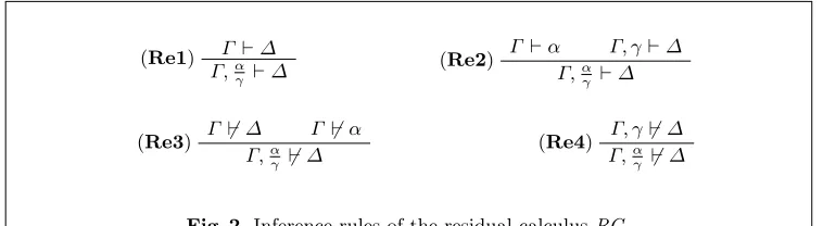
(respec-tively does not) follow from𝑊 using the residues𝑅. The rules ofRC comprise of the inference rules from Fig. 2 together with the rules ofLK andAC. How-ever, the use of rules from LK and AC is restricted to purely propositional (anti)sequents. For this calculus, Bonatti and Olivetti [5] showed:

𝛤 ⊢𝛥 (Re1)

𝛤,𝛼 𝛾 ⊢𝛥

𝛤 ⊢𝛼 𝛤, 𝛾⊢𝛥 (Re2)

𝛤,𝛼𝛾 ⊢𝛥

𝛤 ∕⊢𝛥 𝛤 ∕⊢𝛼 (Re3)

𝛤,𝛼 𝛾 ∕⊢𝛥

𝛤, 𝛾∕⊢𝛥 (Re4)

𝛤,𝛼 𝛾 ∕⊢𝛥

Fig. 2.Inference rules of the residual calculusRC.

Theorem 6 (Bonatti, Olivetti [5]). The residual calculus RC is sound and complete, i.e., for all default theories ⟨𝑊, 𝑅⟩ with 𝑅⊆ ℒres _{and all 𝛥⊆ ℒ,}

1. ⟨𝑊, 𝑅⟩ ⊢𝛥is derivable in RC if and only if ⋁

𝛥∈𝐶𝑙(𝑊, 𝑅); 2. ⟨𝑊, 𝑅⟩⊬_{𝛥is derivable in RC if and only if} ⋁

𝛥 /∈𝐶𝑙(𝑊, 𝑅).

To bound the lengths of proofs in this calculus we exploit the property that residues only have to be used at a certain level and are not used to deduce any formulae afterwards (cf. Lemma 3). Using this we prove that the complexity of

Lemma 7. There exist a polynomial 𝑝 and a constant 𝑐 such that 𝑠RC(𝑛) ≤

𝑝(𝑛)⋅𝑠LK(𝑐𝑛) and 𝑡RC(𝑛)≤𝑝(𝑛)⋅𝑡LK(𝑐𝑛).

Proof. The proof consists of two parts. First we will show the bounds stated above for sequents. In the second part we will then show that antisequents even admit polynomial-size proofs inRC.

Assume first that we want to derive the sequent⟨𝑊, 𝑅⟩ ⊢𝛥, where𝑊, 𝛥⊆ ℒ

and 𝑅 ={𝑟1, . . . , 𝑟𝑘} is a set of residues with𝑟𝑖 = 𝛼_𝛾𝑖𝑖. Let 𝑅′ ⊆𝑅 be minimal with respect to the size ∣𝑅′∣ such that ⟨𝑊, 𝑅′⟩ ⊢ 𝛥. We may w.l.o.g. assume that 𝑅′ _={𝑟

1, . . . , 𝑟𝑘′} and 𝑘′ ≤𝑘. Furthermore, by Lemma 3, we may assume that the rules 𝑟𝑖 are ordered in the way they are applied when computing the sets𝐶𝑖. In particular, this means that for each 𝑖= 1, . . . , 𝑘′,

𝑊 ∪ {𝛾1, . . . , 𝛾𝑖−1} ⊢𝛼𝑖

is a true propositional sequent for which we fix an LK-proof 𝛱𝑖. We augment

𝛱𝑖 by 𝑘′−𝑖applications of rule (Re1) to obtain

⟨𝑊 ∪ {𝛾1, . . . , 𝛾𝑖−1},{𝑟𝑖+1, . . . , 𝑟𝑘′}⟩ ⊢𝛼_𝑖 .

Let us call the proof of this sequent𝛱_𝑖′.

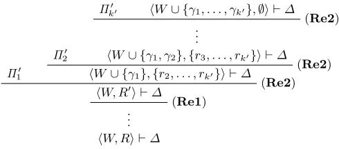
The proof tree depicted in Fig. 3 for deriving⟨𝑊, 𝑅⟩ ⊢𝛥unfurls as follows. We start with an LK-proof for the sequent 𝑊 ∪ {𝛾1, . . . , 𝛾𝑘′} ⊢ 𝛥 and then apply𝑘′-times the rule (Re2) in the step

⟨𝑊∪ {𝛾1, . . . , 𝛾𝑖−1},{𝑟𝑖+1, . . . , 𝑟𝑘′}⟩ ⊢𝛼𝑖 ⟨𝑊∪ {𝛾1, . . . , 𝛾𝑖},{𝑟𝑖+1, . . . , 𝑟𝑘′}⟩ ⊢𝛥

⟨𝑊∪ {𝛾1, . . . , 𝛾𝑖−1},{𝑟𝑖, . . . , 𝑟𝑘′}⟩ ⊢𝛥

to reach⟨𝑊, 𝑅′_{⟩ ⊢𝛥. To derive the left prerequisite we use the proof𝛱}′

𝑖. Finally we use 𝑘−𝑘′ applications of the rule (Re1) to get⟨𝑊, 𝑅⟩ ⊢𝛥.

Π′

1

Π′

2

Π𝑘′′ ⟨𝑊∪ {𝛾1, . . . , 𝛾𝑘′},∅⟩ ⊢𝛥

(Re2) ..

.

⟨𝑊∪ {𝛾1, 𝛾2},{𝑟3, . . . , 𝑟𝑘′}⟩ ⊢𝛥

(Re2) ⟨𝑊∪ {𝛾1},{𝑟2, . . . , 𝑟𝑘′}⟩ ⊢𝛥

(Re2) ⟨𝑊, 𝑅′_{⟩ ⊢𝛥}

(Re1) ..

. ⟨𝑊, 𝑅⟩ ⊢𝛥

Fig. 3.Proof tree for the sequent⟨𝑊, 𝑅⟩ ⊢𝛥in the residual calculus.

Our proof for ⟨𝑊, 𝑅⟩ ⊢ 𝛥 uses at most (𝑘′ _{+ 1)⋅𝑡}

LK(𝑛) + 𝑘

′_(𝑘′₊₁₎

2 +𝑘

steps, i.e.,𝑡RC(𝑛)≤ 𝒪(𝑛⋅𝑡LK(𝑛) +𝑛2). Each sequent is of linear size. Hence,

𝑠RC(𝑛)≤𝑝(𝑛)⋅𝑠LK(𝑛) for some polynomial𝑝.

In the second part of the proof we have to show that any true antisequent has anRC-proof of polynomial size, thus concluding the proof. Let⟨𝑊, 𝑅⟩⊬_𝛥

and let {𝑖1, . . . , 𝑖ℓ}=𝐼 ⊆ {1, . . . , 𝑘} be a set of maximal cardinality such that 〈

𝑊 ∪∪

𝑖∈𝐼{𝛾𝑖} 〉

⊬_{𝛥and let𝐼}′_{={𝑖ℓ+1, . . . , 𝑖𝑘}={1, . . . , 𝑘} ∖𝐼.}

Because of ⟨𝑊, 𝑅⟩ ⊬ _{𝛥, the set 𝐼 contains all indices 𝑖 with 𝛼𝑖 ∈ 𝐶𝑙(𝑊).}

Therefore, for each 𝑗 ∈ 𝐼′ we have 𝑊 ∪∪

𝑖∈𝐼{𝛾𝑖} ⊬ 𝛼𝑗. We fix a polynomial-size AC-proof 𝛱𝑗 of this antisequent. Augmenting these proofs with ℓ appli-cations of (Re4) we obtain a proof 𝛱_𝑗′ of 〈

𝑊,∪

𝑖∈𝐼{𝑟𝑖} 〉

⊬ _{𝛼𝑗. Similarly, as}

〈

𝑊 ∪∪

𝑖∈𝐼{𝛾𝑖} 〉

⊬_{𝛥we get a polynomial-size proof𝛱}′

𝑘+1of

〈

𝑊,∪

𝑖∈𝐼{𝑟𝑖} 〉

⊬_𝛥.

Now, the proof for⟨𝑊, 𝑅⟩⊬_{𝛥ends with the following application of (Re3)}

〈

𝑊,{𝑟𝑖1, . . . , 𝑟𝑖𝑘−1}

〉

⊬_𝛥 〈

𝑊,{𝑟𝑖1, . . . , 𝑟𝑖𝑘−1}

〉

⊬_𝛼𝑖 𝑘

⟨𝑊,{𝑟𝑖1, . . . , 𝑟𝑖𝑘}⟩⊬𝛥

More generally, for all choices of𝑠, 𝑡withℓ < 𝑠 < 𝑡≤𝑘+ 1 we use the (Re3)-step

〈

𝑊,{𝑟𝑖1, . . . , 𝑟𝑖𝑠−1}

〉

⊬_𝛼𝑖 𝑡

〈

𝑊,{𝑟𝑖1, . . . , 𝑟𝑖𝑠−1}

〉

⊬_𝛼𝑖 𝑠

⟨𝑊,{𝑟𝑖1, . . . , 𝑟𝑖𝑠}⟩⊬𝛼𝑖𝑡

where we set 𝛼𝑘+1 = ⋁𝛥. After all these steps, it remains to derive the

an-tisequents ⟨𝑊,{𝑟𝑖1, . . . , 𝑟𝑖ℓ}⟩ ⊬ 𝛼𝑖𝑡 for ℓ < 𝑡 ≤ 𝑘+ 1. But for these we have

already built the proofs 𝛱_𝑡′. Therefore, we have constructed an RC-proof of

⟨𝑊, 𝑅⟩⊬_{𝛥which apart from the AC-proofs𝛱𝑡}′ _{uses only𝒪(𝑘}2_{) applications of}

(Re3) and (Re4). As each antisequent in the proof is of linear size, we obtain a polynomial-sizeRC-proof of ⟨𝑊, 𝑅⟩⊬_{𝛥. ⊓⊔}

Let us remark that while the RC-proof of ⟨𝑊, 𝑅⟩ ⊢𝛥 in Fig. 3 is tree-like, this is not true for our dag-like RC-proof of ⟨𝑊, 𝑅⟩ ⊬ _{𝛥 constructed in the}

second part of the proof of Lemma 7.

4 Proof Complexity of Credulous Default Reasoning

Now we turn to the analysis of Bonatti and Olivetti’s calculus for credulous default reasoning. An essential ingredient of the calculus are provability con-straints which resemble a necessity modality. Provability constraints are of the formL𝛼or¬L𝛼with𝛼∈ ℒ. A set𝐸⊆ ℒsatisfies a constraintL𝛼if𝛼∈𝑇 ℎ(𝐸). Similarly,𝐸 satisfies¬L𝛼 if𝛼∕∈𝑇 ℎ(𝐸).

We can now describe the calculus BOcred of Bonatti and Olivetti [5] for

credulous default reasoning. Acredulous default sequent is a 3-tuple ⟨𝛴, 𝛤, 𝛥⟩, denoted by 𝛴;𝛤∣∼𝛥, where 𝛤 = ⟨𝑊, 𝐷⟩ is a default theory, 𝛴 is a set of

provability constraints and𝛥 is a set of propositional sentences. Semantically, the sequent 𝛴;𝛤∣_∼𝛥 is true, if there exists a stable extension 𝐸 of 𝛤 which satisfies all of the constraints in𝛴and ⋁

𝛥∈𝐸. The calculusBOcred uses such

sequents and extendsLK,AC, and RC by the inference rules in Fig. 4. For this calculus Bonatti and Olivetti [5] show the following:

Theorem 8 (Bonatti, Olivetti [5]). BOcred is sound and complete, i.e., a

credulous default sequent is true if and only if it is derivable in BOcred.

We now investigate lengths of proofs inBOcred. Our next lemma shows that

𝛤 ⊢𝛥 (cD1)

; 𝛤∣∼𝛥

𝛤 ⊢𝛼 𝛴; 𝛤∣∼𝛥

(cD2)

L𝛼, 𝛴; 𝛤∣∼𝛥

𝛤 ∕⊢𝛼 𝛴; 𝛤∣∼𝛥

(cD3)

¬L𝛼, 𝛴; 𝛤∣∼𝛥

where𝛤 ⊆ ℒres _{in rules (cD1), (cD2), and (cD3)}

L¬𝛽𝑖, 𝛴; 𝛤∣∼𝛥

(cD4)

𝛴; 𝛤,𝛼:𝛽1...𝛽𝑛

𝛾 ∣∼𝛥

¬L¬𝛽1. . .¬L¬𝛽𝑛, 𝛴; 𝛤,𝛼_𝛾∣∼𝛥

(cD5)

𝛴; 𝛤,𝛼:𝛽1...𝛽𝑛

𝛾 ∣∼𝛥

Fig. 4.Inference rules for the credulous default calculusBOcred.

Lemma 9. For any function𝑡(𝑛), if RC is𝑡(𝑛)-bounded, then BOcred is𝑝(𝑛)⋅

𝑡(𝑛)-bounded for some polynomial𝑝. The same relation holds for the number of steps in RC and BOcred.

Proof. Let 𝛴;𝛤∣∼𝛥 be a true credulous default sequent. We will construct a

BOcred-derivation of𝛴;𝛤∣∼𝛥starting from the bottom with the given sequent.

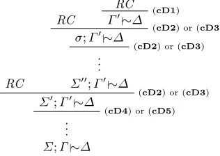
Observe that we cannot use any of the rules (cD1) through (cD3) as long as 𝛤 contains proper defaults with nonempty justification. Thus we first have to reduce all defaults to residues plus some set of constraints using (cD4) or (cD5). As one of these rules has to be applied exactly once for each appearance of some default in 𝛤 we end up with 𝛴′;𝛤′∣∼𝛥, where ∣𝛴′∣ is polynomial in

∣𝛤 ∪𝛴∣and𝛤′ _{is equal to 𝛤 on its propositional part and contains some of the}

corresponding residues instead of the defaults from 𝛤. From this point on we can only use rules (cD2) and (cD3) until we have eliminated all constraints and then finally apply rule (cD1) once. Thus, BOcred-proofs look as shown in

Fig. 5 where RC indicates a derivation in the residual calculus and 𝜎 is the

RC

RC

RC

(cD1₎

𝛤′∣∼𝛥

(cD2_{) or (}cD3₎

𝜎;𝛤′_∣∼𝛥

(cD2_{) or (}cD3₎

.. . 𝛴′′;𝛤′∣∼𝛥

(cD2) or (cD3) 𝛴′;𝛤′∣∼𝛥

(cD4) or (cD5) ..

. 𝛴;𝛤∣_∼𝛥

Fig. 5.The structure of theBOcred-proof in Lemma 9

remaining constraint from 𝛴 after applications of (cD2) or (cD3). Hence we obtain the bounds on 𝑠BOcred and 𝑡BOcred. ⊓⊔

Combining Lemmas 7 and 9 we obtain our main result in this section stating a tight connection between the proof complexity of LK and BOcred.

Theorem 10. There exist a polynomial 𝑝and a constant𝑐such that𝑠LK(𝑛)≤

In the light of this result, proving either non-trivial lower or upper bounds to the proof size of BOcred seems very difficult—as such a result would mean a

major breakthrough in propositional proof complexity (cf. [4, 18]).

4.1 On the Automatizability of BO_cred

Practitioners are not only interested in the size of a proof, but face the more complicated problem to actually construct a proof for a given instance. Of course, in the presence of super-polynomial lower bounds to the proof size this cannot be done in polynomial time. Thus, in proof search the best one can hope for is the following notion of automatizability:

Definition 11 (Bonet, Pitassi, Raz [7]). A proof system 𝑃 for a language

𝐿 isautomatizable if there exists a deterministic procedure that takes as input a string 𝑥 and outputs a 𝑃-proof of 𝑥 in time polynomial in the size of the shortest 𝑃-proof of 𝑥 if 𝑥∈ 𝐿. If 𝑥 ∕∈𝐿, then the behavior of the algorithm is unspecified.

For practical purposes automatizable proof systems would be very desirable. Searching for a proof we may not find the shortest one, but we are guaranteed to find one that is only polynomially longer. Unfortunately, for BOcred there

are strong limitations towards this goal as our next result shows:

Theorem 12. BOcred is not automatizable unless factoring integers is possible

in polynomial time.

Proof. First we observe that automatizability of BOcred implies

automatizabil-ity of Frege systems. For this let 𝜑 be a propositional tautology. By assump-tion, we can construct a BOcred-proof of ∅∣∼𝜑. This BOcred-proof contains an

LK-proof of ∅ ⊢ 𝜑by rule (cD1). As LK is polynomially equivalent to Frege systems [18], we can construct from this LK-proof a Frege proof of 𝜑in poly-nomial time. By a result of Bonet, Pitassi, and Raz [7], Frege systems are not automatizable unless Blum integers can be factored in polynomial time (a Blum integer is the product of two primes which are both congruent 3 modulo 4). ⊓⊔

4.2 A General Construction of Proof Systems for Credulous Default Reasoning

In this section we will explain a general method how to construct proof systems for credulous default reasoning. These proof systems arise from the canonical

Σp

2 algorithm for credulous default reasoning (Algorithm 1). Algorithm 1 first

guesses a generating set𝐺extfor a potential stable extension and then verifies by

the stage construction from Theorem 1 that𝐺ext indeed generates a stable

ex-tension which moreover contains the formula𝜑. Algorithm 1 is aΣp

2 procedure,

i.e., it can be executed by a nondeterministic polynomial-time Turing machine

𝑀 with access to a coNP_{-oracle. The nondeterminism solely lies in line 1 and}

the oracle queries are made in lines 6 and 11 to thecoNP_{-complete problem of}

Algorithm 1 A Σp

2 procedure for credulous default reasoning

Require: ⟨𝑊, 𝐷⟩,𝜑

1: guess𝐷0⊆𝐷and let𝐺ext←𝑊∪ {

𝛾∣𝛼:𝛽𝛾 ∈𝐷0 }

2: 𝐺new←𝑊 3: repeat

4: 𝐺old←𝐺new 5: for all 𝛼:𝛽_𝛾 ∈𝐷do

6: if 𝐺old∣=𝛼and𝐺ext∕∣=¬𝛽then 7: 𝐺new←𝐺new∪ {𝛾}

8: end if

9: end for

10: until𝐺new=𝐺old

11: if 𝐺new=𝐺extand𝐺ext∣=𝜑then 12: return true

13: else

14: return false

15: end if

Algorithm 1 can be converted into a proof system for credulous default reasoning as follows. We fix a propositional proof system 𝑃 and define a proof systemCred(𝑃) for credulous default reasoning where proofs are of the form

⟨𝑊, 𝐷, 𝜑,comp, 𝑞1, . . . , 𝑞𝑘, 𝑎1, . . . , 𝑎𝑘⟩ .

Here comp is a computation of 𝑀 on input ⟨𝑊, 𝐷, 𝜑⟩ and 𝑞1, . . . , 𝑞𝑘 are the queries to IMP during this computation. If the IMP-query 𝑞𝑖 = ⟨𝛹𝑖, 𝜑𝑖⟩ is answered positively, then𝑎𝑖 is a𝑃-proof of

( ⋀

𝜓∈𝛹𝑖𝜓

)

→𝜑𝑖, otherwise𝑎𝑖 is an assignment falsifying this formula. For this proof system we obtain the following bounds:

Theorem 13. Let 𝑃 be a propositional proof system. Then Cred(𝑃)is a proof system for credulous default reasoning with 𝑠𝑃(𝑛)≤𝑠Cred(𝑃)(𝑛)≤ 𝒪(𝑛2𝑠𝑃(𝑛)).

Proof. The first inequality holds because we can use Cred(𝑃) to prove propo-sitional tautologies𝜑 by choosing𝑊 =𝐷=∅.

For the second inequality, we observe that Algorithm 1 has quadratic run-ning time. In particular, a computation of Algorithm 1 contains at most a quadratic number of queries to IMP. Each of these queries is of linear size because it only consists of formulae from the input. If the query is answered positively, then we have to supply a 𝑃-proof and there exists such a 𝑃-proof of size ≤𝑠𝑃(𝑛). For a negative answer we just include an assignment of linear size. This yields 𝑠_Cred(𝑃)(𝑛)≤ 𝒪(𝑛2𝑠𝑃(𝑛)). ⊓⊔ Theorem 13 tells us that proving lower bounds for proof systems for cred-ulous default reasoning is more or less the same as proving lower bounds to propositional proof systems. In particular, we get:

5 Lower Bounds for Skeptical Default Reasoning

Bonatti and Olivetti [5] introduce two calculi for skeptical default reasoning. As before, objects are sequents of the form𝛴;𝛤∣_∼𝛥, where𝛴is a set of constraints,

𝛤 is a propositional default theory, and𝛥is a set of propositional formulae. But now, the sequent𝛴;𝛤∣∼𝛥is true, if⋁

𝛥holds in allextensions of𝛤 satisfying the constraints in𝛴.

The first calculus BOskep consists of the defining axioms of LK and AC,

the inference rules of LK, AC, RC, and the rules from Fig. 6. Bonatti and

𝛤 ⊢𝛥 (sD1)

𝛴;𝛤∣∼𝛥

𝛤 ⊢𝛼 (sD2)

¬L𝛼, 𝛴;𝛤∣∼𝛥

𝛤 ∕⊢𝛼 (sD3)

L𝛼, 𝛴;𝛤∣∼𝛥

where𝛤 ⊆ ℒres _{in rules (sD1), (sD2), and (sD3)}

¬L¬𝛽1, . . . ,¬L¬𝛽𝑛, 𝛴;𝛤,𝛼_𝛾∣∼𝛥 L¬𝛽1, 𝛴;𝛤∣∼𝛥 . . . L¬𝛽𝑛, 𝛴;𝛤∣∼𝛥

(sD4)

𝛴;𝛤,𝛼:𝛽1...𝛽𝑛

𝛾 ∣∼𝛥

Fig. 6.Inference rules for the skeptical default calculusBOskep.

Olivetti show that each true sequent is derivable inBOskep,i.e., the calculus is

sound and complete. However, they already remark that proofs in BOskep are

of exponential size in the number of default rules in the sequent. This is due to the residual rules for they cannot be applied unless all defaults with nonempty justifications have been eliminated using rule (sD4).

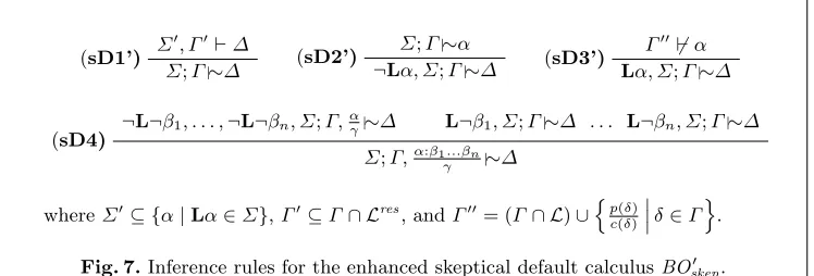
To get more concise proofs, Bonatti and Olivetti [5] suggest an enhanced calculusBO_skep′ where the rules (sD1) to (sD3) are replaced by rules (sD1′) to (sD3′_{) and rule (sD4) is kept (see Fig. 7). Bonatti and Olivetti prove}

sound-ness and completesound-ness forBO_skep′ . Moreover, they show thatBO_skep′ is exponen-tially separated from BOskep, i.e., there exist sequents (𝑆𝑛)𝑛≥1 which require

exponential-size proofs inBOskep but have linear-size derivations inBOskep′ . In

𝛴′_{, 𝛤}′_⊢𝛥

(sD1’)

𝛴;𝛤∣∼𝛥

𝛴;𝛤∣∼𝛼

(sD2’)

¬L𝛼, 𝛴;𝛤∣∼𝛥

𝛤′′_∕⊢𝛼

(sD3’)

L𝛼, 𝛴;𝛤∣∼𝛥

¬L¬𝛽1, . . . ,¬L¬𝛽𝑛, 𝛴;𝛤,𝛼_𝛾∣∼𝛥 L¬𝛽1, 𝛴;𝛤∣∼𝛥 . . . L¬𝛽𝑛, 𝛴;𝛤∣∼𝛥 (sD4)

𝛴;𝛤,𝛼:𝛽1...𝛽𝑛

𝛾 ∣∼𝛥

where𝛴′⊆ {𝛼∣L𝛼∈𝛴},𝛤′⊆𝛤∩ ℒres_{, and𝛤}′′_{= (𝛤∩ ℒ)∪}{𝑝(𝛿) 𝑐(𝛿) 𝛿∈𝛤

} .

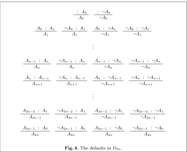
our next result we will show an exponential lower bound to the proof length (and therefore also to the proof size) in the enhanced skeptical calculusBO_skep′ . Theorem 15. The calculus BO_skep′ has exponential lower bounds to the lengths of proofs. More precisely, there exist sequents 𝑆𝑛 of size 𝒪(𝑛) such that every

BO_skep′ -proof of 𝑆𝑛 uses 2𝛺(𝑛) steps. Therefore, 𝑠BO_skep′ (𝑛), 𝑡BO_skep′ (𝑛)∈2𝛺(𝑛).

Proof. We construct a sequence (𝑆𝑛)𝑛≥1= (𝛴𝑛;𝛤𝑛∣∼𝜓𝑛)𝑛≥1 such that for some

constant𝑐, everyBO_skep′ -proof of𝑆𝑛has length at least 2𝛺(𝑛). We choose𝛴𝑛=

∅, 𝜓𝑛 = 𝐴2𝑛, and 𝛤𝑛 = ⟨∅, 𝐷2𝑛⟩, where 𝐷2𝑛 consists of the defaults listed in Fig. 8. The default theory 𝛤𝑛 possesses 2𝑛+1 stable extensions. Observe that each of these contains 𝐴2𝑛, but that each pair of stable extensions differs in truth assigned to the propositional variables 𝐴0, . . . , 𝐴𝑛. We claim that every

: 𝐴0 𝐴0

: ¬𝐴0 ¬𝐴0

𝐴0 : 𝐴1 𝐴1

¬𝐴0 : 𝐴1 𝐴1

𝐴0 : ¬𝐴1 ¬𝐴1

¬𝐴0 : ¬𝐴1 ¬𝐴1

.. .

𝐴𝑛−1 : 𝐴𝑛 𝐴𝑛

¬𝐴𝑛−1 : 𝐴𝑛 𝐴𝑛

𝐴𝑛−1 : ¬𝐴𝑛 ¬𝐴𝑛

¬𝐴𝑛−1 : ¬𝐴𝑛 ¬𝐴𝑛

𝐴𝑛 : 𝐴𝑛−1 𝐴𝑛+1

¬𝐴𝑛 : 𝐴𝑛−1 𝐴𝑛+1

𝐴𝑛 : ¬𝐴𝑛−1 ¬𝐴𝑛+1

¬𝐴𝑛 : ¬𝐴𝑛−1 ¬𝐴𝑛+1

.. .

𝐴2𝑛−2 : 𝐴1 𝐴2𝑛−1

¬𝐴2𝑛−2 : 𝐴1 𝐴2𝑛−1

𝐴2𝑛−2 : ¬𝐴1 ¬𝐴2𝑛−1

¬𝐴2𝑛−2 : ¬𝐴1 ¬𝐴2𝑛−1

𝐴2𝑛−1 : 𝐴0 𝐴2𝑛

¬𝐴2𝑛−1 : 𝐴0 𝐴2𝑛

𝐴2𝑛−1 : ¬𝐴0 𝐴2𝑛

¬𝐴2𝑛−1 : ¬𝐴0 𝐴2𝑛

Fig. 8.The defaults in𝐷2𝑛.

proof of 𝑆𝑛has exponential length in 𝑛. More precisely, we will show that rule (sD4) has to be applied an exponential number of times.

To this end, let𝛱 be a BO_skep′ -proof of 𝐷2𝑛∣∼𝐴2𝑛. We claim that if

𝛴;𝐷, 𝑅∣∼𝐴2𝑛 (1)

is a sequent in𝛱such that𝛴is consistent and there exists an𝑖∈ {𝑛+1, . . . ,2𝑛}

such that 𝐷2𝑛 can be partitioned into three sets 𝐼1,𝐼2,𝐼3 satisfying

2. L¬𝑗(𝛿)∈𝛴 if𝛿∈𝐼2,

3. 𝛿∈𝐷if𝛿 ∈𝐼3, and

4. {𝐴𝑖,¬𝐴𝑖} ∩ {𝑐(𝛿)∣𝛿∈𝐼1}=∅,

then𝛱 has to contain an application of (sD4) to a default rule deriving𝐴𝑖 or

¬𝐴𝑖. Intuitively, the set 𝐼1 contains those default rules that have been applied,

𝐼2 contains those default rules that have been discarded, and 𝐼3 contains the

default rules that have not been used yet. Also note that the fourth condition together with the consistency of 𝛴 implies that 𝐷 still contains default rules with conclusion𝐴𝑖 or¬𝐴𝑖.

To prove this claim, let 𝛴;𝐷, 𝑅∣∼𝐴2𝑛 be a sequent as stated above and

𝑛 < 𝑖 ≤ 2𝑛 be such that {𝐴𝑖,¬𝐴𝑖} ∩ {𝑐(𝛿) ∣ 𝛿 ∈ 𝐼1} = ∅. Suppose that

𝛱 does not contain any applications of (sD4) to default rules deriving 𝐴𝑖 or

¬𝐴𝑖. Consequently,𝛴;𝐷, 𝑅∣∼𝐴2𝑛 is derived by applications of (sD1’), (sD2’), (sD3’) or (sD4) to a default rules not deriving 𝐴𝑖 or ¬𝐴𝑖. We distinguish among the rule which has been applied to derive (1).

(sD1’) Suppose 𝛴;𝐷, 𝑅∣∼𝐴2𝑛 were derived by an application of (sD1’), then

𝛱 had to contain the predecessor𝛴′, 𝑅⊢𝐴2𝑛, where 𝛴′ ⊆ {𝐴𝑘,¬𝐴𝑘 ∣0≤

𝑘 ≤ 𝑛}. By the fourth condition, {𝐴𝑖,¬𝐴𝑖} ∩ {𝑐(𝛿) ∣ 𝛿 ∈ 𝐼1} = ∅. Hence,

𝑅 cannot contain any of the residual rules 𝛼𝑖−1

𝛼𝑖 with𝛼𝑖 ∈ {𝐴𝑖,¬𝐴𝑖}. As 𝛼𝑖

does not occur anywhere else in 𝛴′, 𝑅, the sequent 𝛴′;𝑅∣_∼𝐴2𝑛 cannot be closed.

(sD2’) If 𝛴;𝐷, 𝑅∣∼𝐴2𝑛 were derived by an application of (sD2’), then𝛱 had to contain the predecessor 𝛴′;𝐷, 𝑅∣∼𝛼𝑘, where 𝛼𝑘 ∈ {𝐴𝑘,¬𝐴𝑘} with 0 ≤

𝑘 ≤ 𝑛 and 𝛴′ := 𝛴∖ {¬L𝛼𝑘} (notice that we identify ¬¬𝐴𝑖 and 𝐴𝑖 for simplicity of notation). Suppose that both the sequent 𝛴;𝐷, 𝑅∣∼𝐴2𝑛 and its predecessor 𝛴′;𝐷, 𝑅∣∼𝛼𝑘 were true. Then¬L𝛼𝑘 ∈𝛴 implies that there exists a stable extension not containing 𝛼𝑘, whereas 𝛴′;𝐷, 𝑅∣∼𝛼𝑘 asserts that all stable extensions of𝐷, 𝑅contain𝛼𝑘. From the correctness ofBOskep′

and the consistency of𝛴 ⊇𝛴′we thus obtain a contradiction to the validity of 𝛴′;𝐷, 𝑅∣∼𝛼𝑘.

(sD3’) Similarly, if the sequent𝛴;𝐷, 𝑅∣∼𝐴2𝑛were derived by an application of the rule (sD3’), then 𝛱 contained the sequent𝐷′′, 𝑅⊬_{𝛼𝑙 for some𝛼𝑙 such}

that L𝛼𝑙 ∈ 𝛴, where 𝐷′′ = {

𝑝(𝛿)

𝑐(𝛿)

𝛿 ∈𝐷

}

. Here the set 𝐷′′ is a superset of the residues of the generating defaults of any stable extension satisfying the proof constraints in 𝛴; hence any sentence that does not follow from

𝐷′′ cannot belong to these stable extensions. By the correctness ofBO_skep′ , the ability to prove𝐷′′_{, 𝑅⊬𝛼}

𝑙 would thus imply that no stable extension of

𝛤𝑛 satisfiesL𝛼𝑙. Yet,𝛤𝑛 has a stable extension satisfying any consistent set of proof constraints formed over the propositions in {𝐴𝑖,¬𝐴𝑖 ∣0≤𝑖≤𝑛}. Thus, by the correctness ofBO_skep′ ,𝐷′′_{, 𝑅⊬𝛼}

𝑙 cannot be closed.

(sD4) Suppose that 𝛴;𝐷, 𝑅∣∼𝐴2𝑛 is derived by an application of (sD4) to the default rule 𝛼𝑘−1:𝛼𝑙

𝛼𝑘 ∈ 𝐷 with 𝑛 < 𝑘 ∕= 𝑖 and 𝑙 ∈ {𝑘,2𝑛−𝑘}. Let

𝐷′ :=𝐷∖{𝛼𝑘−1:𝛼𝑙

𝛼𝑘

}

. Then 𝛱 contains the two ancestor sequents

𝛴,¬L¬𝛼𝑙;𝐷′, 𝑅,

𝛼𝑘−1

𝛼𝑘

But neither of these sequents contains a residual rule deriving 𝐴𝑖 or ¬𝐴𝑖, while both contain less default rules. Thus iterating this argument until no default rules deriving𝐴𝑗 or¬𝐴𝑗 for𝑗∕=𝑖remain yields a contradiction. Concluding, the containment of𝛴;𝐷, 𝑅∣∼𝐴2𝑛 in𝛱 enforces an application of (sD4) to a default rule 𝛿 with conclusion 𝐴𝑖 or ¬𝐴𝑖. This yields the ances-tor sequents𝛴,¬L¬𝛼2𝑛−𝑖;𝐷′, 𝑅,𝛼_𝛼𝑖−_𝑖1∣∼𝐴2𝑛and𝛴,L¬𝛼2𝑛−𝑖;𝐷′, 𝑅∣∼𝐴2𝑛, where

𝐷′ _{:=𝐷∖ {𝛿}. The latter of these still satisfies the requirements of (1). Thus,}

by the same arguments as above, 𝛱 has to contain an application of (sD4) (to a default rule 𝛼𝑖−1:¬𝛼2𝑛−𝑖

¬𝛼𝑖 ). Each of these applications of (sD4) yields a sequent

satisfying (1) unless for these {𝐴𝑖,¬𝐴𝑖} ∩ {𝑐(𝛿) ∣ 𝛿 ∈ 𝐼1} ∕= ∅ holds for all

𝑛 < 𝑖≤2𝑛; these sequents do, in particular, possess different proof constraints. Summing up, to prove𝐷2𝑛∣∼𝐴2𝑛, 𝛱 has to contain 22𝑛−𝑖+1 applications of (sD4) to default rules with conclusion 𝐴𝑖 or¬𝐴𝑖. Therefore, every proof of𝑆𝑛

has length at least 2𝛺(𝑛). ⊓⊔

We point out that the above argument does not only work against tree-like proofs, but also rules out the possibility of sub-exponential dag-like derivations for 𝐷2𝑛∣∼𝐴2𝑛. The lower bound is obtained from the fact that to derive 𝐴2𝑛, we have to derive a residual rules concluding𝐴𝑖 and a residual rule concluding

¬𝐴𝑖, for each 𝑛 < 𝑖≤2𝑛. These can, by construction of 𝛤𝑛, only be obtained from ancestors with mutually different proof constraints and, in turn, implies mutually disjoint sets of ancestor sequents.

6 Conclusion

In this paper we have shown that with respect to lengths of proofs, proof systems for credulous default reasoning and for propositional logic are very close to each other. Although deciding credulous default sequents is presumably harder than deciding tautologies (the former is Σp

2-complete [14], while the latter is

complete for coNP_{), the difference disappears when we want to prove these}

objects (Sect. 4.2).

For skeptical reasoning this is less clear. While skeptical default reasoning has polynomially bounded proof systems if and only if this holds for TAUT, we leave open whether this equivalence extends to other bounds. However, in the light of our exponential lower bound for BO_skep′ (Theorem 15), searching for natural proof systems for skeptical default reasoning with more concise proofs will be a rewarding task for future research.

In this direction Bonatti and Olivetti [5] themselves introduced two rules to supplement their enhanced calculus. These are the cut rule

𝛴;𝛤∣∼𝛼 𝛴;𝛤, 𝛼∣∼𝛥

(Cut)

𝛴;𝛤∣∼𝛥

and the following version of the rule (sD4)

𝛴0, 𝛴;𝛤,𝛼_𝛾∣∼𝛥 𝛴1, 𝛴;𝛤∣∼𝛥 . . . 𝛴𝑛, 𝛴;𝛤∣∼𝛥

(sD4′)

𝛴;𝛤,𝛼:𝛽1...𝛽𝑛

where𝛴𝑖=L¬𝛽𝜋(𝑖),¬L¬𝛽𝜋(𝑖+1), . . . ,¬L¬𝛽𝜋(𝑛) for an arbitrary permutation𝜋

of {1, . . . , 𝑛}. While it is not hard to see that our lower bound in Theorem 15 still remains true if we add (sD4′) to BO_skep′ , we leave open the problem to show super-polynomial lower bounds in the presence of the cut rule.

Acknowledgments

The first author wishes to thank Neil Thapen for interesting discussions on the topic of this paper during a research visit to Prague. We also thank the anony-mous referees of the conference version of this article for helpful comments.

References

1. G. Amati, L. C. Aiello, D. M. Gabbay, and F. Pirri. A proof theoretical approach to default reasoning I: Tableaux for default logic. Journal of Logic and Computation, 6(2):205–231, 1996.

2. G. Antoniou. A tutorial on default logics.ACM Comput. Surv., 31(4):337–359, 1999. 3. O. Beyersdorff, A. Meier, S. M¨uller, M. Thomas, and H. Vollmer. Proof complexity

of propositional default logic. In Proc. 13th International Conference on Theory and Applications of Satisfiability Testing, volume 6175 ofLecture Notes in Computer Science, pages 30–43. Springer-Verlag, Berlin Heidelberg, 2010.

4. P. A. Bonatti. A Gentzen system for non-theorems. Technical Report CD/TR 93/52, Christian Doppler Labor f¨ur Expertensysteme, 1993.

5. P. A. Bonatti and N. Olivetti. Sequent calculi for propositional nonmonotonic logics.

ACM Transactions on Computational Logic, 3(2):226–278, 2002.

6. M. L. Bonet, S. R. Buss, and T. Pitassi. Are there hard examples for Frege systems? In P. Clote and J. Remmel, editors,Feasible Mathematics II, pages 30–56. Birkh¨auser, 1995. 7. M. L. Bonet, T. Pitassi, and R. Raz. On interpolation and automatization for Frege

systems. SIAM Journal on Computing, 29(6):1939–1967, 2000.

8. M. Cadoli and M. Schaerf. A survey of complexity results for nonmonotonic logics.Journal of Logic Programming, 17(2/3&4):127–160, 1993.

9. S. A. Cook and R. A. Reckhow. The relative efficiency of propositional proof systems.

The Journal of Symbolic Logic, 44(1):36–50, 1979.

10. J. Dix, U. Furbach, and I. Niemel¨a. Nonmonotonic reasoning: Towards efficient calculi and implementations. In Handbook of Automated Reasoning, pages 1241–1354. Elsevier and MIT Press, 2001.

11. U. Egly and H. Tompits. Proof-complexity results for nonmonotonic reasoning. ACM Transactions on Computational Logic, 2(3):340–387, 2001.

12. D. Gabbay. Theoretical foundations of non-monotonic reasoning in expert systems. In

Logics and Models of Concurrent Systems, pages 439–457. Springer-Verlag, Berlin Heidel-berg, 1985.

13. G. Gentzen. Untersuchungen ¨uber das logische Schließen. Mathematische Zeitschrift, 39:68–131, 1935.

14. G. Gottlob. Complexity results for nonmonotonic logics.Journal of Logic and Computa-tion, 2(3):397–425, 1992.

15. P. Hrubeˇs. On lengths of proofs in non-classical logics.Annals of Pure and Applied Logic, 157(2–3):194–205, 2009.

16. E. Jeˇr´abek. Frege systems for extensible modal logics. Annals of Pure and Applied Logic, 142:366–379, 2006.

17. E. Jeˇr´abek. Substitution Frege and extended Frege proof systems in non-classical logics.

Annals of Pure and Applied Logic, 159(1–2):1–48, 2009.

19. S. Kraus, D. J. Lehmann, and M. Magidor. Nonmonotonic reasoning, preferential models and cumulative logics. Artificial Intelligence, 44(1–2):167–207, 1990.

20. D. Makinson. General theory of cumulative inference. InProc. 2nd International Work-shop on Non-Monotonic Reasoning, pages 1–18. Springer-Verlag, Berlin Heidelberg, 1989. 21. V. W. Marek and M. Truszczy´nski.Nonmonotonic Logics—Context-Dependent Reasoning.

Springer-Verlag, Berlin Heidelberg, 1993.

22. R. Reiter. A logic for default reasoning. Artificial Intelligence, 13:81–132, 1980.

23. V. Risch and C. Schwind. Tableaux-based characterization and theorem proving for default logic. Journal of Automated Reasoning, 13(2):223–242, 1994.