Mapping the core mass function on to the stellar initial mass function:
multiplicity matters
K. Holman,
1‹S. K. Walch,
1,2S. P. Goodwin
3and A. P. Whitworth
11School of Physics and Astronomy, Cardiff University, Queens Buildings, The Parade, Cardiff CF24 3AA, UK 2Max-Planck-Institut f¨ur Astrophysik, Karl-Schwarzschild-Str. 1, D-85741 Garching, Germany
3Department of Physics and Astronomy, University of Sheffield, Hicks Building, Housfield Road, Sheffield S3 7RH, UK
Accepted 2013 April 22. Received 2013 April 9; in original form 2013 February 4
A B S T R A C T
Observations indicate that the central portions of the present-day prestellar core mass function (hereafter CMF) and the stellar initial mass function (hereafter IMF) both have approximately log-normal shapes, but that the CMF is displaced to higher mass than the IMF by a factor F∼4±1. This has led to suggestions that the shape of the IMF is directly inherited from the shape of the CMF – and therefore, by implication, that there is a self-similar mapping from the CMF on to the IMF. If we assume a self-similar mapping, it follows (i) thatF =NO/η, whereηis the mean fraction of a core’s mass that ends up in stars andNOis the mean number of stars spawned by a single core; and (ii) that the stars spawned by a single core must have an approximately log-normal distribution of relative masses, with universal standard deviation
σO. Observations can be expected to deliver ever more accurate estimates ofF, but this still leaves a degeneracy betweenηandNO, and σOis also unconstrained by observation. Here we show that these parameters can be estimated by invoking binary statistics. Specifically, if (a) each core spawns one long-lived binary system, and (b) the probability that a star of mass Mis part of this long-lived binary is proportional toMα, current observations of the binary frequency as a function of primary mass,b(M1), and the distribution of mass ratios,pq, strongly favourη∼1.0±0.3, NO∼4.3±0.4, σO∼0.3±0.03 andα∼0.9±0.6; η >1 just means that, between when its mass is measured and when it finishes spawning stars, a core accretes additional mass, for example from the filament in which it is embedded. If not all cores spawn a long-lived binary system, db/dM1<0, in strong disagreement with observation; conversely, if a core typically spawns more than one long-lived binary system, thenNOandηhave to be increased further. The mapping from CMF to IMF is not necessarily self-similar – there are many possible motivations for a non-self-similar mapping – but if it is not, then the shape of the IMF cannot be inherited from the CMF. Given the limited observational constraints currently available and the ability of a self-similar mapping to satisfy them, the possibility that the shape of the IMF is inherited from the CMF cannot be ruled out at this juncture.
Key words: binaries: general – stars: formation – stars: luminosity function, mass function – stars: statistics.
1 I N T R O D U C T I O N
Understanding the processes that determine the initial mass function (IMF), and why these processes appear to vary little with environ-ment and metallicity, is one of the main challenges in star formation (e.g. Elmegreen, Klessen & Wilson 2008). Recent observations of prestellar cores (i.e. the dense, gravitationally bound condensations in molecular clouds that are presumed to be destined to form in-dividual stars or multiple systems) suggest that such cores have a mass function very similar in shape to the IMF, but shifted to higher
E-mail: [email protected]
addition, we still need to understand how an individual core maps into an individual star or multiple system, and to what extent this process can really be viewed as statistically self-similar.
The IMF has been evaluated by Kroupa (2001) and Chabrier (2003, 2005). Chabrier finds that the IMF is well fitted with a log-normal function merging into a power law at high masses. Theoret-ical models and simulations of turbulent fragmentation suggest that the CMF may also approximate to a log-normal function merging into a power law at high masses (Padoan & Nordlund 2002; Padoan et al. 2007; Hennebelle & Chabrier 2008, 2009).
However, these theories do not address the origins of stellar mul-tiplicity. It is therefore timely to formulate the mapping between core mass and star mass using simple distribution functions, so that the additional constraints imposed by stellar multiplicity can be taken into account. It turns out that these additional constraints can be accommodated quite easily, but strongly favour a mapping in which each core typically spawnsNO∼4 stars, with quite high efficiency,η∼1; the individual stars spawned by a core have a log-normal mass distribution with standard deviationσO∼0.3, and
two of them end up in a long-lived binary system. The probability that a star with massMends up in a long-lived binary system is approximately proportional toM.
In the interests of simplicity, we ignore the high-mass power-law parts of the mass functions, and concentrate on the log-normal parts, since these are the parts that are best constrained by observation, and they can be described with just two parameters: a logarithmic1
mean and standard deviation. Therefore, our conclusions are most pertinent to the mass range where this log-normal form appears to be an acceptable approximation, say 0.03–3 M. However, it should be noted that our conclusions are not significantly changed if the high-mass power-law tail is included; this simply makes the maths more laborious and less precise. For a detailed discussion of the IMF and the eight parameters that may be needed to describe it more completely, the reader is referred to Bastian, Covey & Meyer (2010). We limit our consideration of multiplicity statistics to (i) the binary frequency as a function of primary mass, and (ii) the distribution of mass ratios (for systems with Sun-like and M-dwarf primaries), again because these appear to be the multiplicity statistics that are most robustly constrained by observation. For the purpose of this paper, brown dwarfs are counted as stars.
In Section 2, we present the definitions and assumptions under-lying our model. In Section 3, we present the observational data we will use to estimate the model parameters. In Section 4, we describe the consequences of the model, using simple arguments; this discussion preempts the results of the more rigorous statistical analysis that follows. In Section 5, we describe how stellar statistics are evaluated for a particular model using Monte Carlo integration; and in Section 6, we define the parameter we use to measure the quality of fit between a model and the observations. In Section 7, we describe the Markov chain procedure for identifying the best-fitting model parameters, and in Section 8 we present the results. In Section 9, we discuss the results and relate them to previous work, and in Section 10 we summarize our main conclusions.
2 T H E M O D E L 2.1 Assumptions
If one accepts that most stars are formed in cores (see e.g. Bressert et al. 2010), the model has only four assumptions.
1Throughout, all logarithms are to base 10.
Assumption I. The central portions of the CMF and the IMF are both log-normal.
Assumption II. The mapping between them is statistically self-similar, which means that the distribution of therelativemasses of the stars spawned by a single core must also be log-normal.
Assumption III. When a core forms more than one star, two of these stars end up in a binary system that is sufficiently long lived to contribute to the statistics of binaries in the field. All the rest ultimately end up as singles.
Assumption IV. The relative probability that a star with massM
ends up in a long-lived binary system is proportional toMα. We note that these assumptions are not made because we believe that they are necessarily true, but because they are simple, and because it turns out that they suffice to fit all the observational constraints that currently appear to be robust.
In addition, we note that the long-lived binary systems that con-tribute to the field statistics are probably not the only ones that form in a core cluster, but simply the ones that survive its dissolution and subsequent tidal perturbations (e.g. Kroupa 1995). There is evi-dence (e.g. K¨ohler et al. 2008; Chen et al. 2013) that the multiplicity is much higher for young stars in some star formation regions than for older stars in the field, and also includes a significant proportion of higher order multiples. However, by the time stars arrive in the field, many of these systems are likely to have been destroyed, and the wider systems will continue to suffer attrition due to stochastic tidal perturbations.
In other words, there are two very different time-scales involved in the mapping. The mean number of stars spawned by a core (NO) and the mean total mass of the stars spawned by a core (hence the efficiency,ηO) are – ignoring stellar mass-loss, accretion, mass
exchange and mergers – determined by processes that terminate once the core disperses, after at most a few mega-years. In contrast, the binary statistics are never completely settled. They evolve most rapidly during the birth throes of the core cluster (the NO stars formed from a single core) and during its dispersion, but they then evolve further due to interactions with other stars in the same large-scale cluster (here presumed to be an ensemble of stars formed from an ensemble of cores), and they continue to evolve, after the large-scale cluster dissolves, due to interactions with the ever changing background gravitational field (e.g. tidal perturbations from passing stars and molecular clouds). However, these latter perturbations are rare, and given that the typical field star has been in the field for many giga-years, its binary statistics should by now be well defined. Our model does not concern itself with the details of the dynamical evolution of the stars spawned by a single core; it simply focuses on the properties of systems that survive to populate the field, posits that each core typically spawns just one such system and shows that the observed binary statistics are reproduced well if this system tends to comprise two of the more massive stars spawned by the core. Other binary systems, and higher multiples, are spawned by a core, but we presume that they are disrupted on a time-scale1 Gyr. One would expect the binary systems surviving in the field to be on average more massive and closer than the ones that have been disrupted.
2.2 Input parameters
Table 1 summarizes the six model input parameters, namely the logarithmic mean,μC, and standard deviation,σC, of the CMF; the
Table 1. Input parameters regulating a single Monte Carlo integration, and the ranges of values admitted by the Markov chain. The prior for the Markov chain is that, within these ranges, all values are equally probable.MCis the mass of a core and{Mn}nn==N1 are the masses of the stars formed from a single core.
Parameter Identity Minimum Maximum
μC Arithmetic mean of log10(MC/M) −0.2 +0.2
σC Standard deviation of log10(MC/M) 0.3 0.7
η Mean star formation efficiency in core=nn==N1 {Mn}/MC 0.0 2.0
NO Mean number of stars formed in core 1.0 7.0
σO Standard deviation of log10(Mn/M) 0.0 0.5
α Dynamical biasing parameter, d ln(pM)/d ln(M) −2.0 5.0
stars spawned by a core; and the dynamical biasing parameter,α. There are direct observational constraints onμCandσC, but not, as
yet, onη,NO,σOandα.
We note that values ofηgreater than unity are admissible because, between the time when the mass of a core is estimated and added to the CMF, and the time when its star formation is complete, the core can, and almost certainly does, grow in mass, for example by accretion along the filament in which it is embedded (e.g. Smith et al. 2011). By the same token it is not necessary that all the stars spawned by a core form simultaneously. Indeed, numerical simulations suggest that some of the stars spawned by a core start to condense out of the filamentary material accreting on to the core, and may only reach the core as it starts to disintegrate (e.g. Bate 2012; Girichidis et al. 2012)
In addition, non-integer values ofNO are admissible. In such cases, we adopt the simple device of dividing cores between the integer values that bracketNO. Thus, for example,NO=2.2 means that 80 per cent of cores haveN =2 and 20 per cent haveN =3. Apart from this device, we do not allow any variance in the input parameters, because to do so introduces extra input parameters, but does not significantly improve, or even alter, the fits obtained.
2.3 Output parameters
Given the four assumptions listed above, and values for the six input parameters, we can predict the IMF (which, being log-normal, is characterized by a logarithmic mean,μS, and a logarithmic standard
deviation,σS), the binary frequency as a function of primary mass, b(M1), and the distributions of mass ratio for systems with Sun-like
and M-dwarf primaries,pq(M1). Our objective is to use observations
of these output parameters [μS,σS,b(M1),pq(M1)] to constrain the
model input parameters (μC,σC,η,NO,σO,α).
3 O B S E RVAT I O N A L DATA
Table 2 summarizes the expectation values,VX, uncertainties,UX,
and weights,WX, according to the different observational
param-eters,X, that the model seeks to predict. The weights determine the influence that different observed quantities exert on the overall quality of fit of a model (see Section 6), and by design they add up to unity.
For the mean and standard deviation of the IMF, μS andσS,
[image:3.595.64.530.508.733.2]we use values informed by Chabrier (2005), and since these two
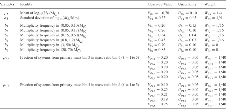
Table 2. Output parameters characterizing the observed IMF and binary statistics (two left-hand columns), and parameters regulating the quality of the fit of a model to the observations (three right-hand columns). Column 1 gives the name of the parameter in the model, and Column 2 its identity. Column 3 gives the observed value (V) of this parameter, and Column 4 its uncertainty (U). Column 5 gives the weight (W) according to fitting the observed value.MSis the mass of a star from the whole ensemble of stars formed in a single Monte Carlo integration. The sources for
the observational data are given in Section 3.
Parameter Identity Observed Value Uncertainty Weight
μS Mean of log10(MS/M) VμS= −0.70 UμS=0.10 WμS=1/4
σS Standard deviation of log10(MS/M) VσS=0.55 UσS=0.05 WσS=1/4
b1 Multiplicity frequency in (0.05, 0.10) M Vb1=0.20 Ub1=0.15 Wb1=1/16
b2 Multiplicity frequency in (0.05, 0.17) M Vb2=0.26 Ub2=0.10 Wb2=1/16
b3 Multiplicity frequency in (0.15, 0.60) M Vb3=0.34 Ub3=0.04 Wb3=1/16
b4 Multiplicity frequency in (0.8, 1.2) M Vb4=0.45 Ub4=0.03 Wb4=1/16
b5 Multiplicity frequency in (3, 50) M Vb5=0.70 Ub5=0.10 Wb5=0
b6 Multiplicity frequency in (20, 70) M Vb6=0.85 Ub6=0.10 Wb6=0
p3, Fraction of systems from primary-mass bin 3 in mass-ratio bin(=1 to 5) Vp3,1=0.20 Up3,1=0.05 Wp3,1=1/40 Vp3,2=0.20 Up3,2=0.05 Wp3,2=1/40
Vp3,3=0.20 Up3,3=0.05 Wp3,3=1/40
Vp3,4=0.20 Up3,4=0.05 Wp3,4=1/40
Vp3,5=0.20 Up3,5=0.05 Wp3,5=1/40
p4, Fraction of systems from primary-mass bin 4 in mass-ratio bin(=1 to 5) Vp4,1=0.10 Up4,1=0.03 Wp4,1=1/40
Vp4,2=0.25 Up4,2=0.05 Wp4,2=1/40
Vp4,3=0.21 Up4,3=0.05 Wp4,3=1/40
Vp4,4=0.19 Up4,4=0.04 Wp4,4=1/40
quantities appear to be quite well constrained by observation, we give them both a high weight,WμS=WσS=1/4.
For the binary frequencies we consider six primary-mass bins. Binm=1 (the lowest mass bin) represents the results of Close et al. (2003), bin 2 those of Basri & Reiners (2006), bin 3 those of Janson et al. (2012), bin 4 those of Raghavan et al. (2010), bin 5 those of Preibisch et al. (1999) and bin 6 those of Mason et al. (1998). For evaluating the quality of the fit, we give the first four bins equal weights,Wbi =1/16, i=1 to 4, so that their combined weight is 1/4. The last two bins are given zero weight, because the stars in these bins are not strictly field stars.2Therefore, these
two bins should not influence the choice of the best-fitting model. They are included because – notwithstanding – the predictions of the best-fitting model agree with them well (see Fig. 3).
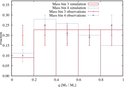
For the distribution of mass ratios,q, we consider only primary-mass binsm=3 and 4, since these are the ones with relatively ro-bust mass-ratio statistics (Raghavan et al. 2010; Reggiani & Meyer 2011; Janson et al. 2012). In both primary-mass bins, the distribu-tion of mass ratios appears to be flat (Reggiani & Meyer 2011). We follow convention by allocating the mass ratios to five equal bins,= 1 to 5, so that binaccommodates values in the range 0.2(−1)<q≤0.2. For primary-mass bin 3, Janson et al. (2012) conclude that, when allowance is made for selection effects, the distribution of mass ratios is flat, and therefore we simply set all the expectation values toVp3, =0.20, and all the uncertainties to
Up3,=0.05. For primary-mass bin 4, we adopt expectation values
and Poisson uncertainties from Raghavan et al. (2010). For all 10 primary-mass/mass-ratio bins, we allocateWpm,=1/40, so that their combined weight is 1/4.
4 S I M P L E I N F E R E N C E S
In Section 8, we present the results of a Markov chain Monte Carlo analysis. Here we present simple arguments to preempt the main results of that analysis.
4.1 The shift between the IMF and the CMF
The mean mass of the stars that form from a given core is related to the mass of the core by the efficiency,η(the fraction of the core’s mass that ends up in stars), divided by the number of stars formed from the coreNO. Hence, the factor by which the peak of the CMF exceeds the peak of the IMF is given by
F≡10(μC−μS) = NO
η . (1)
If we adoptμS= −0.6±0.05 (from Chabrier 2003) andμC =
0.0±0.1 (from, e.g., Enoch et al. 2006, 2008; Young et al. 2006; K¨onyves et al. 2010), we haveF4±1 , whence
NO = F η(4±1)η . (2)
4.2 Raising the degeneracy betweenNOandη
The degeneracy betweenNOandηcan be raised by considering the binary statistics. Two essential features of the binary statistics in the field are that – very roughly – the number of single-star systems is comparable with, but somewhat larger than, the number of binary
2The last two bins concern binaries with relatively high-mass short-lived
primaries in the Orion nebula cluster (Preibisch et al. 1999) and a mixture of systems in clusters, associations and the field (Mason et al. 1998).
systems,andthe binary frequency is an increasing function of pri-mary mass (db/dM1>0). The influence of these constraints can
be understood with the following Gedankenexperiment. Suppose (purely for the sake of argument, and averaged over all masses) that 60 per cent of systems are single and 40 per cent are binary. This can be achieved in two ways.
(i)NO=1.4. In this case, 60 per cent of cores have N =1 and spawn singles, whilst 40 per cent of cores haveN =2 and spawn binaries. This gives 0.26η0.44. However, it means that the components of binary systems are on average less massive than single stars, and therefore the binary fraction is a decreasing function of primary mass, which is the opposite of what is observed. (ii)NO=3.5. In this case, each core spawns a binary system, but 50 per cent haveN =3 so they spawn one extra single star, and the remaining 50 per cent have N =4 and therefore spawn two extra single stars. This gives 0.7η1. Moreover, provided
α >0, the components of binary systems are now, on average, more massive than the single stars, and consequently the binary fraction is an increasing function of primary mass, as observed.
There is therefore a strong preference for the larger value ofNO, to ensure that db/dM1>0.
4.3 Standard deviation of the relative masses of the stars spawned by a single core
Since the mapping of the CMF on to the IMF involves the convolu-tion of a log-normal CMF with a log-normal distribuconvolu-tion of relative stellar masses, the logarithmic standard deviation of the IMF,σS, is
obtained by adding the logarithmic standard deviation of the CMF,
σC, and the logarithmic standard deviation of the relative stellar
masses,σO, in quadrature,
σ2 S =σ
2 C + σ
2
O. (3)
A corollary of equation (3) is that – for a self-similar mapping – the logarithmic standard deviation of the IMF cannot be smaller than the logarithmic standard deviation of the CMF,
σS ≥σC. (4)
In interpreting this inequality, one must recognize that the log-normal CMF we are discussing here is one that represents a very large region embracing a representative ensemble of star formation regions; the log-normal CMFs inferred for individual star formation regions can – and apparently do – have a range of means and logarithmic standard deviations, but together they cannot have a logarithmic standard deviation greater than that of the IMF and still admit a self-similar mapping. Since observations suggestσC∼σS,
this in turn implies thatσOcannot bevery large.
4.4 Mass ratios
Observations (Raghavan et al. 2010; Reggiani & Meyer 2011; Janson et al. 2012) suggest that the distributions of mass ratio for binary systems having Sun-like and M-dwarf primaries are both flat. In our model, this means first thatσOcannot bevery small,3
otherwise the range of stellar masses formed in a single core would be too narrow to produce low-qsystems; and secondly thatαcannot
3It turns out that finding a value ofσ
Othat is both small enough to
be too large, otherwise the low-mass stars would have little chance of pairing up with the high-mass ones to produce low-qsystems.
5 M O N T E C A R L O I N T E G R AT I O N
For a single model (i.e. a fixed combination of the input parameters,
μC, σC, η,NO, σO, α), we evaluate the stellar statistics as follows.
First, a core mass,MC, is obtained by generating a Gaussian
random deviate,G, on (−∞,+∞), and setting
MC=10(μC+GσC)M. (5)
Next, ifNOis a non-integer, a value forNis obtained by generating a linear random deviate,L, on (0, 1), and putting
N =
INT(NO), whenL≥NO−INT(NO);
INT(NO)+1, whenL<NO−INT(NO). (6)
OtherwiseN =NO. Then the masses of theN stars spawned by this core can be obtained by generating Gaussian random deviates,
G, on (−∞,+∞), and computing
MS= MCη
N 10GσO. (7)
IfN ≥2, the integrated probability of each possible pairing of these stars (starnwith starn) is computed,
Pn,n =
ν=n
ν=1
ν=n
ν=ν+1
Mα ν Mνα
ν=N− 1
ν=1
ν=N
ν=ν+1
Mα νMνα
. (8)
Finally, a linear random variate,L, on (0, 1) is generated, and the pairing whose integrated probability is just aboveLis selected.
This is repeated until a total of 107 stars have been created.
Then the mean and standard deviation of the IMF,μSandσS, are
computed (using the logarithms of the stellar masses). For each star that falls in one of the mass bins defined in Table 2, we note whether it is the primary in a binary system, the secondary in a binary system or a single star; and, if it is a primary, we also note which mass-ratio bin the binary falls in. If mass binmcontainsPmprimaries andSm
singles, the corresponding binary frequency4is
bm = P Pm
m+Sm. (9)
If mass-ratio binof mass binmcontainsCmsystems, the corre-sponding mass-ratio probability is
pm,= CPm m .
(10)
The model can then be compared with the observational data.
4We refer the reader to Reipurth & Zinnecker (1993) for a discussion of
different measures of multiplicity and their various merits. The one defined in equation (9) is in effect the multiplicity frequency, but we refer to it as the binary frequency because we are only considering binaries. As pointed out by Hubber & Whitworth (2005), the multiplicity frequency has the nice property that it is insensitive to whether a binary system is actually a higher order multiple. We note parenthetically that there are in general other stars in each mass bin that are secondaries, but these do not explicitly affect the calculation of thebm.
6 Q UA L I T Y O F F I T
For each model (i.e. each Monte Carlo integration with a given set of input parameters,μC, σC, η,NO, σO, α), the quality of fit,Q,
is given by a sum of terms,
QX= − WX(X−VX)
2
U2
X ,
(11)
representing how well the model prediction for output parameter
X(≡μS,σS,bm[form = 1, 2, 3, 4],pm[form = 3, 4; = 1, 2, 3, 4, 5]) matches with the observational constraints (see Ta-ble 2). The overall quality of fit for a given model is then
Q(μC, σC, η,NO, σO, α)=
−WμS(μS−VμS)
2
U2
μSt
− WσS(σS−VσS)
2 U2 σS − m=4 m=1
Wbm(bm−Vbm)2 U2 bm − m=4 m=3 =5 =1
Wpm,(pm,−Vpm,)2 U2
pm,
. (12)
The first two terms on the right-hand side of equation (12) measure the ability of the model to reproduce the observed IMF (with an overall weighting of 50 per cent); the third term (involving a single summation) measures its ability to reproduce the observed binary frequency as a function of primary mass (with an overall weighting of 25 per cent); and the fourth term (involving a double summa-tion) measures its ability to reproduce the distributions of mass ratio for systems having Sun-like and M-dwarf primaries (with an over-all weighting of 25 per cent). A notionover-ally perfect fit corresponds toQ=0, and|Q|can be interpreted as the number of standard deviations by which the model departs from a perfect fit.
7 M A R K OV C H A I N 7.1 Range ofμCandσC
Herschel has allowed much more robust evaluations of the CMF. For example, K¨onyves et al. (2010) obtain (μC, σC) = (−0.22,
0.42) and (−0.05, 0.30) in – respectively – the entire Aquila field and the main Aquila subfield. Previously, Enoch et al. (2006) have estimated (μC, σC) = (−0.05± 0.25, 0.50± 0.10) in Perseus,
Young et al. (2006) have estimated (μC,σC)=0.3±0.7, 0.5±
0.4) in Ophiuchus and Enoch et al. (2008) have estimated (μC, σC)=0.00±0.04, 0.30±0.03) for an ensemble of cores from
Perseus, Serpens and Ophiuchus.
However, all these evaluations are convolved with a number of uncertainties. In particular, the use of grey-body fits to estimate mean dust temperatures, the mass opacity coefficients needed to convert fluxes into masses and the distances assumed for the star-formation regions all introduce uncertainty into the derived masses, and hence into theμC-values. σC-values may be somewhat less
susceptible to these factors, but are affected by the fact that the cores on the low-mass side of the log-normal tend to be close to the completeness limit. Furthermore, we are here concerned with the values of μC and σC for the totality of all star-forming cores,
rather than those for a single region.
consequences of takingμC-values outside this range, in Section 8.
ForσCwe restrict the Markov chain to values ofσCin the range
0.3< σC< 0.7. This choice is informed by the range of
obser-vationally inferred values, and by the fact thatσCcannot exceedσS.
7.2 Range ofηandNO
We restrict the Markov chain to values ofηin the range 0< η < 2, and values ofNOin the range 1≤NO≤7. Evidently, if a core accretes very rapidly on the way to forming stars, higherηvalues are possible, but this turns out to be unlikely. The arguments presented in Section 4.2 suggest that higher values ofNOare inadmissible – unless each core spawns more than one long-lived binary,andthe efficiency is increased still further (see Section 4.1).
7.3 Range ofσOandα
We restrict the Markov chain to values ofσOin the range 0< σO <0.5, on the grounds thatσOhas to be smaller thanσS, and is
probably also smaller thanσC.
We restrict the Markov chain to values ofαin the range−2<
α <5. This choice is informed by numerical work on the disso-lution of small-Nclusters (e.g. van Albada 1968a,b; McDonald & Clarke 1993; Sterzik & Durisen 1998; Hubber & Whitworth 2005, and references therein), which suggests that, if the dissolution of a core cluster involves pure gravitational interaction between the stars, a single long-lived binary is the most likely outcome and it usually comprises the two most massive stars, which impliesα 1. Conversely, if there is dissipation – for example, because the stars are attended by massive discs (McDonald & Clarke 1995) – other pairings become more likely, which implies a smallerαvalue. Flat mass-ratio distributions translate into a preference for smallα.
7.4 Markov chain
The ranges detailed above define the input parameter space, and our prior is that all values in these ranges are equally probable. The Markov chain then starts at an arbitrary point in this space, and makes a biased random walk around the space. The components of a step are generated from Gaussian distributions. A step is always taken ifQ=QNEW−QOLD>0 (i.e. if it results in an improve-ment to the fit). IfQ<0, the code generates a linear random deviate,L, on (0, 1), and only takes the step ifQ>ln(L) (i.e. steps that produce a deterioration in the fit are less likely to be taken the larger the deterioration). The size of a step is scaled so that roughly half of all putative steps are not taken.
8 R E S U LT S
From the Markov chain, there is a single well-definedQpeak in the parameter space explored, and the best fit is obtained with
μC= −0.03 ±0.10, (13)
σC=0.47± 0.04, (14)
η=1.01± 0.27, (15)
NO=4.34 ± 0.43, (16)
σO=0.30 ±0.03, (17)
α=0.87 ± 0.64, (18)
Q= −0.33, (19)
i.e. 0.33σ overall difference between the model and the observa-tions.
The parameters of the CMF (μC,σC) are compatible with those
obtained from observation, althoughμChas a rather large
uncer-tainty, and we return to this point below.
The efficiency (η) is much higher than the values normally esti-mated (e.g. Alves et al. 2007).ηis also only just compatible at the high end of the range calculated theoretically by Matzner & McKee (2000), but in their model these high values arise in cores that are intrinsically flattened (so that outflows can escape without sweep-ing up much core mass), rather than as a consequence of formsweep-ing many stars. High notional efficiencies may be an indication that cores grow in mass whilst they collapse and fragment to form stars (e.g. Smith et al. 2011).
The mean number of stars formed from a single core (NO) is also higher than the values normally invoked. Mathematically this follows from the large η(see equation 1), but physically it also derives – inevitably, in a self-similar mapping – from the need to form binaries with a frequency that increases with primary mass (see discussion in Section 4.2).
The spread of stellar masses from a single core cluster (σO=
0.29±0.07) is such that if the stars are paired randomly, between 33 and 56 per cent of the resulting systems have mass ratio below 0.5. Thus, in order to produce a flat distribution of mass ratios, the dynamical biasing parameter should not be too large, and this is what the model infers (α=0.6±1.0).
In Fig. 1, we plot those values ofQgenerated along the Markov chain that exceed−1 (i.e. those models that deliver output parame-ters that are collectively within 1σof the observations), against the different model input parameters. These plots show that the best-fitting model input parameters are all well defined, apart fromμC.
Fortunately,μC is already quite well constrained by observation,
and likely to become better constrained in the future. IfμC were
increased, the efficiency,η, would have to be reduced proportion-ately (or each core would have to produce more than one long-lived binary) – and vice versa.
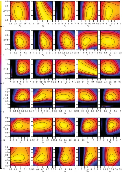
Fig. 2 illustrates howQvaries on planes through the best-fitting solution, i.e. if just two of the model input parameters are varied. These plots are generated with a regular two-dimensional grid of models, and 107stars per model. On each row, the ordinate is the
same for all five plots, and the abscissa cycles through the remaining five input parameters. From the plots in the first row, we see that
μCis weakly constrained, and also, from the second plot along this
row, that ifμCis increased,ηmust be reduced proportionately. In
all other cases, a horizontal scan of the plots in a row reveals that the parameter concerned (the ordinate) is very well, and uniquely, constrained by the observations.
Fig. 3 presents the binary frequency as a function of primary mass, for the best-fitting model, generated using 107stars, along with the
observational data used to constrain the model. We reiterate that we do not use the two higher mass points, but only the four lower mass points. Notwithstanding, the model fits all six points well.
Figure 1. TheQ-values for all models along the Markov chain that haveQ>−1, plotted againstμC,σC,η,NO,σOandα.
9 D I S C U S S I O N 9.1 Critique of the model
The critical assumption of the model is that each core spawns, on average, exactly one long-lived binary system, i.e. one binary system that survives to populate the field. If this assumption were relaxed, in the sense that a core might spawn more than one long-lived binary system (say, on average,Bbinary systems), thenηand
NOwould have to be increased (in proportion toB). Conversely, if not all cores were to spawn a binary system,ηandNOwould have to be reduced, but it would then become impossible to reproduce the variation of binary frequency with primary mass,b(M1) – unless one
were to introduce an additional parameter to allow the efficiency to be much higher for cores that spawn binaries than for those that do not.
If the observed estimate for the overall binary frequency of low-mass field stars [i.e. binaries with primaries in the range (0.02, 2.0) M] were to increase, this would reduceNO, and consequently
η. For example, if the observed overall binary frequency of low-mass field stars were increased to 0.5, the model would requireNO∼3 andη∼0.8±0.2.
It is difficult to see how the various standard deviations could change much, unlessσSis very different from the Chabrier (2005)
value. IfσSwere larger,σCandσOcould also be larger, and vice
versa.
If the distribution of mass ratios were skewed in favour of systems with comparable mass, i.e. dpq/dq>0, thenσOwould need to be
reduced, and/orαincreased (more dynamical biasing).
9.2 Previous theoretical work
Some of the consequences of a self-similar mapping are explored by Clarke (1996), but with different distribution functions and less emphasis on observational constraints.
Swift & Williams (2008) develop a similar model to ours, but one which includes a power-law extension to the CMF at high masses, based on the analysis of Padoan & Nordlund (2002), and which invokes somewhat different model parameters. They explore the consequences of varying the prescriptions for generating multiple systems, and for subfragmentation of a core, but their work differs from ours in that they do not explore in depth the question of multiplicity and its variation with primary mass, and they do not
draw any firm conclusions on the efficiency, or on the number of stars spawned by a single core.
Goodwin et al. (2008) explore the consequences of multiplicity for the mapping from the CMF into the IMF, and in particular the effect of multiplicity on the extremes of the IMF. Their preferred model presumes that all cores spawn multiple systems, with the number of stars in a system increasing very slightly with the mass of the progenitor core (the model is therefore not strictly self-similar), and it has quite a low efficiency,ηO=0.27. They do not explore the
issue of how such systems might subsequently evolve to produce singles, so they cannot exploit the observed variation of binary fraction with primary mass.
Goodwin & Kouwenhoven (2009) demonstrate that the mapping from a log-normal CMF into an approximately log-normal system mass function (SMF) and from the SMF into an approximately log-normal IMF admits a wide range of prescriptions for (i) how the efficiency varies with the core mass (η(MC)), (ii) whether the
probability that a core spawns a single or a binary depends on its mass [effectivelyN(MC)] (iii) and the distribution of mass ratios in
such binaries. This concurs with our conclusion (see Section 9.3) that, whilst there are many theoretical arguments for allowing the input parameters of the mapping to depend on the core mass (thereby rendering the mapping non-self-similar), the effect on the IMF is so subtle that these dependences cannot usefully be constrained by the existing observations.
9.3 Additional model parameters
We have considered the following refinements to the model. How-ever, none of them is justified, since none of them, either individ-ually or in combination, produces a significant improvement to the fit; in respect of items (ii), (iii) and (iv), Goodwin & Kouwenhoven (2009) reached essentially the same conclusion, but on the basis of a very different model and less restrictive observational constraints. Necessarily, all these refinements would corrupt the self-similarity of the mapping.
(i) We have explored models in which the lifetime of a prestellar core (i.e. the time during which a prestellar core is detected as such) depends on its mass according totC∝MCχt. Negative values of χtskew the IMF towards high masses because low-mass cores are over-represented in the CMF. Conversely, positive values ofχtskew
Figure 2. Iso-Qplots on principal planes through the best-fitting model. In each row the ordinate (vertical axis) is the same model input parameter, from top to bottom in the orderμC,σC,η,NO,σOandα. Along each row, the abscissa (horizontal axis) cycles through the remaining model input parameters, in the
Figure 3. The boxes represent the observational estimates of multiplicity frequency in different primary-mass intervals, as detailed in the text, and summarized in Table 2. The error bars represent the observational uncer-tainties. The dashed line shows the multiplicity frequency as a function of primary mass for the best-fitting model. The unruly points at largeM1are
due to small-number statistics.
Figure 4. The distribution of mass ratios for binaries having primaries in mass bins 3 and 4. The plotted symbols with error bars represent the observationally inferred expectation values and uncertainties: orange plus signs for mass bin 3, and blue crosses for mass bin 4. The histograms represent the model results: orange solid line for mass bin 3, and dotted blue line for mass bin 4.
over-represented in the CMF. There is no consensus on this. Hatchell & Fuller (2008) have argued that more massive cores evolve faster than less massive ones, and are therefore under-represented in the CMF; this might be taken into the reckoning withχt= −0.25.
Con-versely, Clark, Klessen & Bonnell (2007) have argued that massive cores being more diffuse have longer lifetimes, and are therefore over-represented in the CMF; on the basis of a simple free-fall ar-gument, and Larson’s scaling relations, this might be taken into the reckoning withχt= +0.25.
(ii) We have explored models in which the efficiency of star formation in a prestellar core depends on its mass according to
ηO∝M
χη
C . This is equivalent to including feedback from massive
stars. Star formation is promoted by feedback from massive stars ifχη is positive, and suppressed ifχηis negative. However, it is not known what the sense of feedback from massive stars is, on the scale of a single core.
(iii) We have explored models in which the number of stars formed from a prestellar core depends on its mass according to
NO∝MχN
C . Negative values of χN (a) skew the IMF towards
high masses, and (b) increase the multiplicity frequency of high-mass stars and reduce the multiplicity frequency of low-high-mass stars. Positive values ofχN have the opposite effects. It is difficult to believe thatN does not increase with core mass (positiveχN). However, this would completely undermine the original argument for a self-similar mapping between CMF and IMF, namely that the high-mass slopes of the CMF and IMF appear to be indistin-guishable. Moreover, in practice, the observational constraints can more easily accommodate the effects of negativeχN. Either way, non-zeroχN-values are not actually needed to fit the observational constraints we have invoked.
(iv) We have explored models in which the logarithmic range of stellar masses formed from a prestellar core depends on its mass according toσO∝MCχσ. It is probably the case that only positive
values ofχσ could be justified (i.e. higher mass cores spawning a greater logarithmic spread of stellar masses), but this is not needed to fit the observational constraints. Moreover, it suppresses the high-mass end of the IMF, which – in this purely log-normal model – is already too low.
(v) We have explored the possibility that there is some vari-ance in, for example,NO, so that whenNO=3 (say) not all cores spawn exactly three stars. However, first this introduces an addi-tional model parameter, which should be avoided if possible, and secondly it makes no significant difference to the results, unless the variance is extremely large, so we do not include it in the basic model.
We reiterate that we are not arguing that these additional effects do not occur in nature. We are simply pointing out (a) that they are not justified by the currently available observational constraints, that is, one can obtain a good fit to the observations without them; and (b) that they would corrupt a self-similar mapping.
1 0 C O N C L U S I O N S
We have developed a simple model to describe the mapping of the CMF on to the IMF.
(i) The model has four assumptions: the central portions of the CMF and IMF are both log-normal; the mapping from the CMF on to the IMF is self-similar; if a core forms more than one star, two of the stars end up in a long-lived binary; and the probability of a star of massMbeing in this binary is proportional toMα.
(ii) The model has six input parameters:μCandσCare the
loga-rithmic mean and standard deviation of the log-normal CMF;ηOis
the efficiency (i.e. the fraction of a core’s mass that ends up in new stars);NOis the mean number of stars spawned by a single core;σO
is the standard deviation of the log-normal distribution of relative stellar masses spawned by a single core; andαis the dynamical biasing parameter.
(iii) This model is able to fit the observed IMF, the ob-served binary frequency as a function of primary mass and the observed distributions of mass ratio for bina-ries having Sun-like and M-dwarf primaries. The best fit requires μC= −0.03±0.10, σC=0.47±0.04, η=1.01±
0.27, NO=4.34±0.43, σO=0.30±0.03 and α = 0.87 ±
0.64 . It fits the observations to within 0.25σ.
[image:9.595.45.284.308.474.2]self-similarity, there is a simple mapping that fits the observational constraints well and therefore – on the basis of Occam’s razor – should be given consideration.
Moreover, if the mapping is not (at least, approximately) self-similar, then the notion that the shape of the IMF is inherited from the CMF must be abandoned.
Either way, there is a question to be answered beyond understand-ing the origin of the CMF:eitherwhy is the mapping self-similar
orwhy does the mapping, despite not being self-similar, produce an IMF with the same shape as the CMF?
The self-similar model suggests that the efficiency of star forma-tion within a prestellar core is significantly higher (ηO1.0±0.3)
than has previously been proposed (e.g.ηO∼0.3; Alves et al. 2007).
It also suggests that most stars, including singles, are born in small groups of approximately four. This contrasts with the conclusion of Lada (2006) that most stars, being single, are born in isolation. In-terestingly, Nakamura, Takakuwa & Kawabe (2012) have recently reported evidence that prestellar cores are more fragmented than had previously been thought. If cores spawn many stars, we may see multiple outflows from some cores (e.g. Wu, Takakuwa & Lim 2009), but these outflows do not have to disperse a large fraction of the core’s initial mass, and can simply punch holes in the residual envelope.
AC K N OW L E D G E M E N T S
We thank Cathie Clarke, Thijs Kouwenhoven, Mike Meyers and Peter Coles for useful discussions that helped to improve this paper. We gratefully acknowledge the support of the UK STFC, via a doctoral training account (KH) and a rolling grant (APW; PP/E000967/1). SKW gratefully acknowledges the support of the DFG Priority Programme No. 1573. SKW, SPG and APW gratefully acknowledge the support of the Marie Curie CONSTELLATION Research Training Network.
R E F E R E N C E S
Alves J., Lombardi M., Lada C. J., 2007, A&A, 462, L17 Basri G., Reiners A., 2006, AJ, 132, 663
Bastian N., Covey K. R., Meyer M. R., 2010, ARA&A, 48, 339 Bate M. R., 2012, MNRAS, 419, 3115
Bressert E. et al., 2010, MNRAS, 409, L54 Chabrier G., 2003, PASP, 115, 763
Chabrier G., 2005, in Corbelli E., Palla F., Zinnecker H., eds, Astrophysics and Space Science Library, Vol. 327, The Initial Mass Function 50 Years Later. Springer, Dordrecht, p. 41
Chen X. et al., 2013, ApJ, 768, 110
Clark P. C., Klessen R. S., Bonnell I. A., 2007, MNRAS, 379, 57 Clarke C. J., 1996, MNRAS, 283, 353
Close L. M., Siegler N., Freed M., Biller B., 2003, ApJ, 587, 407 Elmegreen B. G., Klessen R. S., Wilson C. D., 2008, ApJ, 681, 365 Enoch M. L. et al., 2006, ApJ, 638, 293
Enoch M. L., Evans N. J., II, Sargent A. I., Glenn J., Rosolowsky E., Myers P., 2008, ApJ, 684, 1240
Girichidis P., Federrath C., Banerjee R., Klessen R. S., 2012, MNRAS, 420, 613
Goodwin S. P., Kouwenhoven M. B. N., 2009, MNRAS, 397, L36 Goodwin S. P., Nutter D., Kroupa P., Ward-Thompson D., Whitworth A. P.,
2008, A&A, 477, 823
Hatchell J., Fuller G. A., 2008, A&A, 482, 855 Hennebelle P., Chabrier G., 2008, ApJ, 684, 395 Hennebelle P., Chabrier G., 2009, ApJ, 702, 1428 Hubber D. A., Whitworth A. P., 2005, A&A, 437, 113 Janson M. et al., 2012, ApJ, 754, 44
Johnstone D., Bally J., 2006, ApJ, 653, 383
Johnstone D., Wilson C. D., Moriarty-Schieven G., Joncas G., Smith G., Gregersen E., Fich M., 2000, ApJ, 545, 327
Johnstone D., Fich M., Mitchell G. F., Moriarty-Schieven G., 2001, ApJ, 559, 307
K¨ohler R., Neuh¨auser R., Kr¨amer S., Leinert C., Ott T., Eckart A., 2008, A&A, 488, 997
K¨onyves V. et al., 2010, A&A, 518, L106 Kroupa P., 1995, MNRAS, 277, 1491 Kroupa P., 2001, MNRAS, 322, 231 Lada C. J., 2006, ApJ, 640, L63
Mason B. D., Gies D. R., Hartkopf W. I., Bagnuolo W. G., Jr, ten Brummelaar T., McAlister H. A., 1998, AJ, 115, 821
Matzner C. D., McKee C. F., 2000, ApJ, 545, 364 McDonald J. M., Clarke C. J., 1993, MNRAS, 262, 800 McDonald J. M., Clarke C. J., 1995, MNRAS, 275, 671 Motte F., Andre P., Neri R., 1998, A&A, 336, 150
Motte F., Andr´e P., Ward-Thompson D., Bontemps S., 2001, A&A, 372, L41
Nakamura F., Takakuwa S., Kawabe R., 2012, ApJ, 758, L25 Nutter D., Ward-Thompson D., 2007, MNRAS, 374, 1413 Padoan P., Nordlund Å., 2002, ApJ, 576, 870
Padoan P., Nordlund Å., Kritsuk A. G., Norman M. L., Li P. S., 2007, ApJ, 661, 972
Preibisch T., Balega Y., Hofmann K., Weigelt G., Zinnecker H., 1999, New Astron., 4, 531
Raghavan D. et al., 2010, ApJS, 190, 1
Rathborne J. M., Lada C. J., Muench A. A., Alves J. F., Kainulainen J., Lombardi M., 2009, ApJ, 699, 742
Reggiani M. M., Meyer M. R., 2011, ApJ, 738, 60 Reipurth B., Zinnecker H., 1993, A&A, 278, 81
Simpson R. J., Nutter D., Ward-Thompson D., 2008, MNRAS, 391, 205 Smith R. J., Glover S. C. O., Bonnell I. A., Clark P. C., Klessen R. S., 2011,
MNRAS, 411, 1354
Stanke T., Smith M. D., Gredel R., Khanzadyan T., 2006, A&A, 447, 609 Sterzik M. F., Durisen R. H., 1998, A&A, 339, 95
Swift J. J., Williams J. P., 2008, ApJ, 679, 552 Testi L., Sargent A. I., 1998, ApJ, 508, L91
van Albada T. S., 1968a, Bull. Astron. Inst. Neth., 19, 479 van Albada T. S., 1968b, Bull. Astron. Inst. Neth., 20, 57 Wu P.-F., Takakuwa S., Lim J., 2009, ApJ, 698, 184 Young K. E. et al., 2006, ApJ, 644, 326