Measuring particle concentration in multiphase pipe flow using acoustic backscatter: Generalization of the dual-frequency inversion method.

This is a repository copy of

Measuring particle concentration in multiphase pipe flow using

acoustic backscatter: Generalization of the dual-frequency inversion method.

.

White Rose Research Online URL for this paper:

http://eprints.whiterose.ac.uk/79834/

Version: Accepted Version

Article:

Rice, HP, Fairweather, M, Hunter, TN et al. (3 more authors) (2014) Measuring particle

concentration in multiphase pipe flow using acoustic backscatter: Generalization of the

dual-frequency inversion method. Journal of the Acoustical Society of America, 136 (1).

156 - 169. ISSN 0001-4966

https://doi.org/10.1121/1.4883376

Reuse

Unless indicated otherwise, fulltext items are protected by copyright with all rights reserved. The copyright exception in section 29 of the Copyright, Designs and Patents Act 1988 allows the making of a single copy solely for the purpose of non-commercial research or private study within the limits of fair dealing. The publisher or other rights-holder may allow further reproduction and re-use of this version - refer to the White Rose Research Online record for this item. Where records identify the publisher as the copyright holder, users can verify any specific terms of use on the publisher’s website.

Takedown

If you consider content in White Rose Research Online to be in breach of UK law, please notify us by

Hugh P. Rice

_{, Michael Fairweather, Timothy N. Hunter, Bashar Mahmoud and Simon Biggs}

School of Process, Environmental and Materials Engineering, University of Leeds, Leeds

LS2 9JT, United Kingdom

Jeff Peakall

School of Earth and Environment, University of Leeds, Leeds LS2 9JT, United Kingdom

* Correspondence to [email protected]

Title: Measuring particle concentration in multiphase pipe flow using acoustic backscatter:

generalization of the dual-frequency inversion method

Running title: Measuring particle concentration in pipe flow

Published: Journal of the Acoustical Society of America, July 2014, vol. 136, issue 1, p.

ABSTRACT

A technique, which is an extension of an earlier approach for marine sediments, is

presented for determining the acoustic attenuation and backscattering coefficients of

suspensions of particles of arbitrary materials of general engineering interest. It is

necessary to know these coefficients (published values of which exist for quartz sand only)

in order to implement an ultrasonic dual-frequency inversion method, in which the

backscattered signals received by transducers operating at two frequencies in the

megahertz range are used to determine the concentration profile in suspensions of solid

particles in a carrier fluid. To demonstrate the application of this dual-frequency method to

engineering flows, particle concentration profiles are calculated in turbulent, horizontal

pipe flow. The observed trends in the measured attenuation and backscatter coefficients,

which are compared to estimates based on the available quartz sand data, and the resulting

concentration profiles, demonstrate that this method has potential for measuring the

settling and segregation behavior of real suspensions and slurries in a range of

applications, such as the nuclear and minerals processing industries, and is able to

distinguish between homogeneous, heterogeneous and bed-forming flow regimes. 184

WORDS

Keywords:

acoustic

backscatter;

sediment

transport;

scattering;

attenuation;

instrumentation.

I.

INTRODUCTION

Solid-liquid suspensions are ubiquitous, for example, in the nuclear, minerals and chemical

engineering industries, and the transport and mixing behavior of particles in turbulent,

multiphase flows is of great practical and theoretical interest. In particular, the ability to

measure the concentration of solid particles allows the operator to characterize many

aspects of the flow and suspension properties, such as homogeneity or the presence of a

moving or stationary bed that may cause a blockage or flow constriction, and the efficiency

of mass transport and solids suspension by turbulent mixing. However, in situations where

accessibility is difficult or chemical or radiological hazards are present, it is necessary to

use remote measurement systems that are portable and simple to operate.

Diagnostic methods for the investigation of velocity and particle concentration fields in

settling and non-settling, multiphase suspensions can be categorized as follows (Bachalo,

1994; Powell, 2008; Shukla

et al.

, 2007; Williams

et al.

, 1990): external radiation (

e.g.

ultrasound, X-rays, gamma rays, microwaves, optical light/lasers, neutrons); emitted or

internal radiation (

e.g.

radioactive and magnetic tracers, NMR/MRI); electrical properties

(

e.g.

capacitance, conductance/resistance, inductance and associated tomographic

methods, hot-wire anemometry); physical properties (

e.g.

sedimentation balance,

hydrometric/density measurements, pressure, rheology); and direct methods (

e.g.

physical

sampling, pumping, interruption). Consequently, a number of criteria must be considered

when choosing the most appropriate measurement technique, such as potential hazards,

flow data that are required (Admiraal and García, 2000; Hultmark

et al.

, 2010; Laufer,

1954; Lemmin and Rolland, 1997; Povey, 1997). Acoustic instruments have many

advantages over optical and other systems, most importantly their suitability for

multiphase, sediment-laden, optically opaque flows, as well as their high mobility, ease of

operation, low cost, low signal-processing and calibration requirements and their ability to

measure entire profiles, rather than make only single-point measurements.

Ultrasonic techniques can be used to study a range of processes (Povey, 2006),

e.g.

creaming, sedimentation, phase inversion and other phase transitions, and internal

suspension properties, including

volume fraction (as in this study), particle

compressibility, and particle size (McClements, 1991; Povey, 2013). Such ultrasonic

techniques utilize the speed of sound, attenuation and other, less commonly-used

ultrasonic properties,

e.g.

impedance, angular scattering profile (McClements, 1991), and

are widely used in the study of colloidal suspensions (Challis

et al.

, 2005), marine

sedimentary processes (Thorne and Hanes, 2002), and sedimentation and bed

development in higher-concentration systems (Hunter

et al.

, 2012a; Hunter

et al.

, 2012b;

Hunter

et al.

, 2011). Indeed, Challis

et al

. (2005) are particularly keen to emphasize the

benefits of ultrasonic methods, since one particularly useful capability of such methods is

to interrogate suspensions of much higher concentrations than is possible with optical

methods.

In this study, an acoustic model developed and used extensively by marine scientists

relates the backscattered acoustic signal received by an active piezoelectric transducer to

the properties of the particles in a suspension, and has been employed by a number of

groups (Admiraal and García, 2000; Hunter

et al.

, 2012a). If the acoustic backscatter and

attenuation coefficients of the suspension are known, then the particle concentration

profile can be reconstructed using an explicit dual-frequency inversion method (Hurther

et

al.

, 2011), an extension of the former model that requires echo voltage profiles to be taken

at two ultrasonic frequencies. However, published data for these acoustic coefficients only

exist for quartz-type sand (Thorne and Meral, 2008). The adaptation presented here allows

the backscatter and attenuation coefficients for suspensions of solid particles of any

arbitrary material to be measured empirically, with the aim of applying the dual-frequency

concentration inversion method to suspensions of engineering interest.

The objectives were to measure these coefficients directly for four particle species (two

spherical glass, two non-spherical plastic), compare them to predicted values based on

published quartz-sand data (Thorne and Meral, 2008), and construct concentration profiles

in horizontal pipe flow in order to delineate various flow regimes and quantify the effects

of particle concentration and size, and flow rate, on the segregation behavior of

suspensions.

The structure of the paper is as follows: (a) scattering and absorption processes in

insonified solid-liquid suspensions and an acoustic model for suspended particles are

described in Section II, a novel modification of it for arbitrary types of particle is presented,

measuring the attenuation and backscatter coefficients, and the physical properties of the

particle species used, are described in Section III; and (c) some examples of particle

concentration profiles calculated using the measured coefficients in horizontal pipe flow

II.

THEORY

A.

Acoustic scattering and absorption in suspensions of solid particles

The physical mechanisms present in an insonified suspension can be broadly divided into

two types: (a) scattering,

αsc

, and (b) absorption (

i.e.

conversion of acoustic energy into

heat, sometimes referred to as dissipation). By analogy to optics, these two mechanisms

collectively contribute towards attenuation (classically referred to as extinction) of the

emitted signal in an additive fashion (Dukhin and Goetz, 2002). Absorption mechanisms

can be categorized further, as follows (Babick

et al.

, 1998; Richter

et al.

, 2007): viscous or

visco-inertial,

αvi

; thermal,

αth

; structural,

αst

; electrokinetic,

αel

; and intrinsic,

αin or αw

,

i.e.

those mechanisms that are due to the liquid phase.

A broad summary of the various limiting cases in terms of particle size, ultrasonic

wavelength and other parameters follows, where (Shukla

et al.

, 2010):

=

/ = 2

/ = 2 /

,

[1]

with

k

the wavenumber,

a

the particle size,

ω

the ultrasonic angular frequency,

c

the speed

of sound,

f

the ultrasonic frequency and

λ

the wavelength. The long-, intermediate- and

short-wavelength (or Rayleigh, Mie and geometric, by analogy to optical scattering)

regimes correspond to

ka

≪

1,

ka

~ 1 and

ka

≫

1 (or

λ

≫

a

,

λ

~

a

, and

λ

≪

a

), respectively.

particles, as were used in this study. In particular, thermal (due to particle rigidity),

structural (because there is no aggregation) and electrokinetic absorption are insignificant.

Therefore the total attenuation,

α

, is due to: intrinsic absorption in water,

αw

; viscous

absorption,

αvi

; and scattering,

αsc

(Richards

et al.

, 1996; Thorne and Hanes, 2002), and so

α

=

αw

+

αs

, where the attenuation due to particles is

αs

=

αsc

+

αvi

.

Dukhin and Goetz (2002) note that “sub-micron particles do not scatter ultrasound at all in

the frequency range under 100 MHz” but “only absorb ultrasound”; they also note that

“absorption and scattering are distinctly separated in the frequency domain”, with

absorption dominant at lower frequencies and scattering at higher frequencies. Babick

et

al.

(1998) explain that in the long-wavelength regime (

i.e.

ka

≪

1), “scattering effects are

negligible” and attenuation is mainly due to absorption. However, in the

intermediate-wavelength regime (

i.e. ka

~ 1), dissipation is negligible and “scattering, particularly by

diffraction, increases enormously”.

Attenuation due to particles has generally been found to vary linearly with concentration at

relatively low concentrations with a variety of particle types and fluids (Hay, 1983, 1991;

Hunter

et al.

, 2012a; Richards

et al.

, 1996; Stakutis

et al.

, 1955). In early experiments, Urick

(1948) observed a similar linear dependence, as did Greenwood

et al.

(1993) and Sung

et

al.

(2008) using kaolin-water suspensions. Greenwood

et al.

concluded that scattering was

insignificant in their experiments, since

λ

≫

a

, and found that attenuation was directly

proportional to volume fraction if “there is no interaction between particles”. Moreover, the

linear over a greater range of concentration for lower values of

ka

(Carlson, 2002; Hay,

1991; Shukla

et al.

, 2010). At higher concentrations, however, the backscatter intensity

becomes independent of concentration (Hay, 1991; Hipp

et al.

, 2002).

B.

A model of acoustic backscatter strength

The model described by Thorne and Hanes (2002) and Thorne

et al.

(2011) for marine

sediment was chosen for use in this study because it is simpler to implement than some

other, similar formulations (Carlson, 2002; Furlan

et al.

, 2012; Ha

et al.

, 2011) and has a

firm theoretical basis (Hay, 1991; Kytömaa, 1995; Richards

et al.

, 1996). As a result, it has

previously been employed by a number of groups (Admiraal and García, 2000; Hunter

et

al.

, 2012a; Hurther

et al.

, 2011). In this section, the details of the model are described, with

a view to developing it into a method for determining the properties of suspensions of

arbitrary particles.

The backscattering and attenuation properties of the suspension are embodied in

f

, the

backscatter form function, which “describes the backscattering characteristics of the

scatterers” (Thorne and Buckingham, 2004), and

χ

, which is referred to by Thorne and

Hanes (2002) as “the normalised total scattering cross-section”. The same authors state

that the “sediment attenuation constant is due to absorption and scattering” which “for

noncohesive sediments insonified at megahertz frequencies the scattering component

dominates”. However, this can only be assumed to be true in the short-wavelength regime

For clarity, then,

χ

is hereafter referred to as the normalized total scattering and absorption

cross-section.

f

and

χ

are proportional to (

ka

)

_{and (}

_ka

₎

_{in the Rayleigh (}

_i.e.

long-wavelength) regime, and both tend to constant values at high values of

ka

.

The root-mean-square of the received voltage,

V

, varies with distance from the transducer,

r

, as follows:

=

_,

_[2]

where

α

=

αw

+

αs

, as described earlier;

ks

is the sediment backscatter coefficient and

incorporates the backscattering properties of the particles;

kt

is a system parameter;

M

is

the concentration by mass of suspended particles; and

ψ

is a near-field correction factor

(Downing

et al.

, 1995) that is written as follows:

=

1 + 1.35 + (2.5 )

_{1.35 + (2.5 )}

,

[3]

where

z

=

r

/

rn

and

rn

=

/

;

at

is the radius of the active face of the transducer; and

λ

is

the ultrasound wavelength.

ψ

tends to unity in the far field,

i.e.

when

r

≫

rn

.

αs

and

ks

are as

follows:

$ =

1

% &( ′)

=

〈 〉

, -

.

[5]

where

ξ

is the particle attenuation coefficient, given by:

& =

_{4〈 〉- .}

3〈.〉

[6]

Angled brackets represent the average over the particle size distribution. In particular:

〈 〉 = 0

〈 〉〈

_〈

_{〉 1}

〉

,

[7]

〈.〉 =

〈 〉〈 .〉

_〈

_{〉 .}

[8]

Clearly, both

ks

and

ξ

depend on the particle size distribution and shape and therefore

distance from the transducer in the general case, as do

M

and

αs

. Empirical expressions for

f

and

χ

are known for sandy sediment,

i.e.

quartz-type sand (Thorne and Meral, 2008) and

are as follows:

=

2 01 − 0.35 exp 8− 92 − 1.5

0.7 ; <1 01 + 0.5 exp =− 9

2 − 1.8

2.2 ; ?1

1 + 0.92

,

. =

_{0.95 + 1.282 + 0.252}

0.292

,

[10]

where

2

=

ka

, with

k

the ultrasonic wavenumber and

a

the particle radius.

No such data are available for particle species other than quartz sand, and it was beyond

the remit of this study to construct equivalent expressions for other particle species.

However, for the purpose of validation of the measured values presented later, estimates of

the sediment attenuation coefficient,

ξ

, can be calculated for a particle species with a

known density and mean size using Equations [6] and [10] by setting

a

=

d

/2 and

⟨

χ

⟩

=

χ

(

2

=

ka

), where

d

is the 50

percentile (

i.e.

median) of the measured particle size

distribution (see Section IV.A).

C.

Determination of backscatter and attenuation coefficients in arbitrary suspensions

The objective in this section is to manipulate the expressions in the model presented in

Section II.B in order to derive expressions for the attenuation and backscatter coefficients,

ξh

and

Kh

, which are defined below and are measured in prepared homogeneous

suspensions (hence the

h

subscript), that is, suspensions in which

M

is known and does not

vary with distance. Measured values of

ξh

and

Kh

can then be used within the

dual-frequency concentration inversion method (Hurther

et al.

, 2011), which is described in

suspension of the same particle species. The derivation is followed by a description of the

experimental method for measuring

ξh

and

Kh

in a stirred tank mixer and a summary of the

measured values; lastly, those for

ξh

are compared to theoretical estimates of

ξ

and are

discussed.

First, it is necessary to define the quantity

G

, the range-corrected echo amplitude, such that

D = ln(

)

.

[11]

By multiplying both sides of Equation [2] by

r

, taking the natural logarithm and then the

derivative with respect to distance,

r

, the following expression is obtained:

∂D

∂ =

∂ Hln(

∂

)I =

∂ =ln(

∂

) +

1

2 ln − 2 ($

+ $

)?,

[12]

where the

h

subscript signifies the specific case of homogeneity, which is necessary for the

following stages of the derivation to be valid. This expression is similar to one given by

Thorne and Buckingham (2004). Neither

ks

,

M

nor

αs

depend on

r

, so Equation [4] can be

simplified (

i.e.

αsh

=

ξhM

, where

ξh

is the sediment attenuation constant in the case of a

homogeneous suspension) and the first two terms on the right-hand side of Equation [12]

are zero. It can therefore be rewritten as follows:

∂D

So, the right-hand side of Equation [13] varies linearly with

M

and this expression also

provides a test for homogeneity. By taking the derivative with respect to concentration, an

expression for

ξh

is obtained, as follows:

&

= −

1

₂

_{∂ ∂r = −}

∂ D

1

₂

_{∂ M}

∂

_{∂ Hln(}

∂

)IN.

[14]

This value of

ξ

=

ξh

applies to a suspension in which the particle size distribution and

concentration do not vary spatially. The quantity

K

is defined as the combined backscatter

and attenuation constant, such that, in the general case

O ≡

=

_{exp H2 ($}

K

+ & )I

,

[15]

as described elsewhere (Betteridge

et al.

, 2008; Thorne and Buckingham, 2004; Thorne and

Hanes, 2002). If

ξh

is known, it is then straightforward to find

Kh

,

i.e.

K

measured in a

homogeneous suspension according to the method described above, such that

Kh

≡

kshkt

, for

any combination of particle size and transducer frequency by evaluation of Equation [15],

which also requires that

αw

, the attenuation due to water, be known. In this study, the

expression given by Ainslie and McColm (1998) was rewritten for the case of zero salinity,

as follows:

where

αw

is in Np m

_,

_f

_{is the ultrasonic frequency in MHz and}

_T

_{is the temperature in °C (6}

°C <

T

< 35 °C).

The method for determining the acoustic properties of suspensions of particles described

in this section is novel and can be used with a very wide range of suspensions.

Alternatively, any deviation from the expected behavior can be taken as an indication of

heterogeneity, spatial variation in particle size distribution or significant attenuation.

D.

The Hurther

et al.

dual-frequency concentration inversion method

Concentration inversion methods are algorithms that allow the particle concentration to be

calculated by inversion of a suitable function that relates the concentration to some

measured electromagnetic or acoustic property. They have found wide application in food,

medical and marine science, but have not been exploited to the same extent by engineers,

despite their practical and computational simplicity and low cost relative to other methods

(

e.g.

tomography), and their ability to accurately monitor phase changes, identify critical

transport velocities and delineate flow regimes, for example. In this section, a recent and

very powerful acoustic inversion method is described, and concentration profiles in

turbulent, horizontal pipe flow are constructed using backscatter and attenuation

coefficients that were presented in Section IV.A.

many other implicit and explicit methods that exhibit numerical instability in the far-field

so that errors accumulate with distance from the transducer (Thorne

et al.

, 2011). With the

dual-frequency method, the concentration can be calculated at any measurement point,

independently of that at other points. A description of the method follows. Equation [2] can

be rewritten for the general case, using Equation [4], as follows (Hurther

et al.

, 2011;

Thorne

et al.

, 2011):

( ) = Φ ( )V( )

,

[17]

Φ

( ) ≡ R

T

= R

O

T

,

[18]

V( ) ≡

_{= ( )/Φ ( )}

_.

[19]

If the particle size distribution, and therefore

ξ

and

ks

, do not vary with distance from the

probe, which is a reasonable approximation if the particle species is neutrally buoyant, has

a very narrow size distribution or is very well mixed, the exponent in Equation [19] can be

written as

−4& X ( ′)d ′

(

i.e.

ξ

≠

ξ

(

r

)), and for two transducers that operate at different

frequencies Equation [19] can be rewritten as follows:

V

( ) =

^

,

[20]

Equation [20] by

M

, then taking the natural logarithm and dividing both sides by

ξi

yields a

constant right-hand side, such that

R

V

T

= R

V

T

,

[21]

and rearranging for

M

yields the following:

Yb Ya

= V

V

.

[22]

The explicit expression for particle mass concentration according to the dual-frequency

inversion method is then obtained:

= V

_V

_.

_[23]

In the general case, the particle size distribution and detailed backscatter and attenuation

properties are not known. Experimentally,

J

is evaluated by

J

=

V

_/Φ

_via

_{Equation [19],}

where

V

is the measured voltage and Φ

_{is found using Equation [18], which consists of}

_the

known variables in Equation [2]. Therefore, a minimal requirement for closure is that

ks

and

kt

(or

K

, as in this study),

ξ

and

αw

are known. Whereas

αw

can be calculated using

Equation [16],

K

and

ξ

must be determined experimentally.

ξ

and

ξ

, differ so that

M

can be evaluated accurately from Equation [23]. However, this

condition – which dictates that the smaller of the two frequencies lies in the Rayleigh (

i.e.

low-

ka

) regime in which

ξ

depends very strongly on

ka

, such that

ξ

/

ξ

is “sufficiently

different from unity” (Hurther

et al.

, 2011) – is not so stringent in practice, and is easily

satisfied for particles sizes of

a

< 500 μm and frequencies in the range 1-5 MHz, because

ξ

is

a strong function of

ka

. Indeed, it was found that the two frequencies used in this study, 2

and 4 MHz, were sufficiently different that the ratios of the measured values of

ξ

to

ξ

(

i.e.

ξh

and

ξh

) at

f

= 2 and 4 MHz, respectively, for all four particle species differed

III.

MATERIALS AND METHODS

A.

Materials

The acoustic properties of four particle species were investigated: “Honite 22” and “Honite

16” spherical glass particles, and “Guyblast 40/60” and “Guyblast 30/40” non-spherical

plastic particles (

d

= 41, 77, 468 and 691 μm, respectively). These species were chosen

because they span a range of material properties –

i.e.

size distribution, density and shape –

and therefore exhibit a range of acoustic scattering and absorption properties.

Particle size was measured with

Mastersizer 2000

and

3000

laser diffraction sizers

(Malvern Instruments), density with an

AccuPyc 1300

pycnometer (MicroMeritics) and

particle shape was confirmed by inspection of micrographs from a

BX51

optical microscope

(Olympus). Measured particle size distributions for the glass and plastic species are given

in Figure 1 and Figure 2, respectively. All particle properties are summarized in Table I.

TABLE I: Physical properties of particle species. Species supplied by Guyson International, Ltd. Species Diameter, d50 (μm) Density, ρs (103 kg m-3) Shape

Smaller glass (Honite 22) 41.0 2.45 Spherical

Larger glass (Honite 16) 77.0 2.46 Spherical

Smaller plastic (Guyblast 40/60) 468 1.54 Jagged

Figure 1: Particle size distribution of Honite glass particle species. Data from Mastersizer 2000, Malvern Instruments.

Figure 2: Particle size distribution of Guyblast plastic particle species. Data from Mastersizer 3000, Malvern Instruments. 0 5 10 15 20 25

5 50 500

B.

Operation of the

UVP-DUO

acoustic backscatter system

As discussed in Section I, the capability of ultrasonic systems to interrogate suspensions

with relatively high particle concentrations, along with the many other advantages

described, formed the basis for the choice of the

UVP-DUO

ultrasonic signal processing unit

(Met-Flow, Switzerland). This system was used with two ultrasonic emitter-receiver

transducers operating at 2 and 4 MHz, as the principal diagnostic system in this study, as

the objective was to investigate suspensions with particle concentrations of several percent

by volume. Although intended to be used primarily as an ultrasonic Doppler velocimeter,

the

UVP-DUO

is also a capable acoustic backscatter system and was used as such in this

study: the voltage data themselves were used, rather than a Fourier transform of them,

which yields the Doppler velocity (although the velocity field was used in the positional

calibration of the probes, as described in Section III.D).

In both the stirred mixing vessel and the pipe flow loop, described below, the two probes

were attached to the

UVP-DUO

unit and excited at a voltage of 150 V. For each run,

n

=

2,500 samples of the instantaneous received voltage were collected, with data from each

transducer being taken separately in concurrent runs. Custom-written MATLAB scripts

were used to process the data: the system-applied gain and digitisation constants were

removed, a three-sigma noise filter applied, and the root-mean square (RMS) of the data

C.

Homogeneous suspensions in the stirred tank mixer

As described in Section II.C,

ξh

and

Kh

are the values of

ξ

and

K

when measured in

homogeneous suspensions according to the derivation described in Section II.C. Such

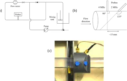
suspensions of known concentrations were prepared in the stirred mixing vessel shown in

Figure 3, which consists of a rotating plastic cylindrical container, the contents of which are

mixed with an impeller connected to a high-speed mixer. Mains water (4 liters) was used as

the fluid at a total depth of around 10 cm. The probes were mounted below the water level

in parallel, with active faces 5 cm from the base of the tank.

(a)

(b)

Figure 3: (a) Stirred mixing vessel schematic and (b) photograph (color online). Mixing tank dimensions: 30 cm width, 30 cm depth. Probes were positioned at about 50 mm from, and perpendicular to, base.

The suspensions were tested for homogeneity by taking physical samples (3 × 60 ml

samples at each concentration, as was the case for the main pipe flow loop described in

more detail below) and comparing them to the total weighed concentration of solids. It was

found that the suspensions prepared in the stirred mixing vessel were very uniformly

~50 mm

mixed, with constants of proportionality between sampled and weighed concentrations for

the Honite 22 (smaller glass), Honite 16 (larger plastic), Guyblast 40/60 (smaller plastic)

and Guyblast 30/40 (larger plastic) species of 0.998, 1.05, 0.987 and 0.863, respectively.

(a)

(b)

(c)

Figure 4: (a) Pipe flow loop schematic, (b) probe mounting geometry schematic and (c) photograph of probes attached to mounting clasp (color online). Inner diameter, D = 42.6 mm; entry length, L = 3.2 m.

A range of nominal particle concentrations were used, from

d

= 0.01 to 10 % by volume,

which corresponds approximately to

Mw

= 0.025 to 250 kg m

_{for the two Honite glass}

species

and

Mw

= 0.015 to 150 kg m

_{for the two Guyblast plastic species. However,}

attenuation was high in suspensions of Guyblast plastic particles at

Mw

≳

15 kg m

_{, and}

this limitation dictated the range over which the coefficients

ξh

and

Kh

were measured (see

Flow meter

Mixing tank

Pump Probes

Flow direction

90°

135°

~15 mm Probes

Section IV.A).

D.

Measurement of settling suspensions in horizontal pipe flow

Data were taken using the same two transducers mounted on a horizontal test section of a

recirculating pipe flow loop (Figure 4) with an inner diameter of

D

= 42.6 mm and a total

capacity of 100 liters (

i.e.

0.1 m

_{). A centrifugal pump, impeller mixer and electromagnetic}

flow meter were used. The probes were mounted at a distance

L

= 3.2 m (

i.e.

75 D) from the

nearest fitting to ensure the flow was fully developed (

i.e.

statistically invariant in the axial

direction) at the test section,

i.e.

at a distance much larger than the necessary entrance

length, even at the highest flow rates (Shames, 2003; Zagarola and Smits, 1998).

The flow loop was filled with suspensions of the same four particle species at several

nominal (weighed) concentrations and run over a range of flow rates. Data from pairs of

runs at the two ultrasonic frequencies were generated and combined (in which

J

,

J

and

M

are functions of distance,

r

, from the transducer), and concentration profiles along a

vertical cross-section were constructed using Equation [23].

As shown in Figure 4, the 2 MHz probe was mounted at 135° to the mean flow direction,

and the 4 MHz probe at 90°, through a clasp on the pipe and through holes in the pipe wall.

The positions of both probes were calibrated: (a) in the case of the 4 MHz probe, by

reference to a strong peak in the echo amplitude corresponding to the position of the lower

the mean axial velocity profile (since the peak coincides with the pipe centerline at high

flow rates), which was also measured. Because the probes were oriented at different angles

to the flow direction, it was necessary firstly to perform a linear transformation of both

datasets onto a common axis (for which the wall-normal distance,

y

, from the upper pipe

wall was chosen). For the same reason, the measurement points for each transducer were

IV.

RESULTS AND DISCUSSION

A.

Measured coefficients and comparison with predictions based on quartz sand data

As specified in Equation [14], in order to calculate

ξh

, it is necessary to know the gradient of

G

with respect to distance,

r

, and mass concentration,

M

. Echo voltage profiles were

recorded using the

UVP-DUO

at several nominal mass concentrations with both

transducers, which were aligned vertically in the stirred mixing vessel, and the data

processed to yield the RMS echo voltage,

V

, from which

G

was calculated according to

Equation [11]. Then, for each run, the gradient,

g

G

/

g

r

, was calculated over the region

r

≈ 24

to 46 mm because it was found that the variation in

G

tended to be most linear over this

region, which was outside the near-field region at both frequencies, for all particles and at

all concentrations of interest. Then, the gradient of

g

G

/

g

r

with respect to

M

was found by

compiling the results over a range of values of

M

according to Equation [14].

Figure 5 shows

G

vs.

r

with the 4 MHz probe for Honite 22, the smaller glass species, at low

and high concentrations (

Mw

= 2.41 and 121.7 kg m

_{), for illustration of the goodness of fit.}

For conciseness, only data for the 4 MHz probe are shown, but the linear fits to the 2 MHz

data were equally good. It should be noted that the peaked nonlinearities in the very near-

and very far-field regions are assumed to be caused by flow around the tip of the probes (

r

< 0.01 m) and reflection from the base of the stirred mixing vessel (

r

> 0.05 m),

respectively. The values of the gradient,

g

G

/

g

r

, over a range of concentrations are shown in

Equation [14]) and goodness of fit with respect to weighed concentration,

Mw

, are also

given. As can be clearly observed from Figure 5, for example,

G

was found to vary very

linearly with respect to

r

for all particle species over the chosen region (24 <

r

< 46 mm), as

the model requires (Equation [13]). Moreover, the variation of

g

G

/

g

r

with respect to

Mw

was also found to be highly linear for all particle species, as shown in Figure 6, for example,

as was also expected (Equation [14]). This kind of linear relationship between

concentration and attenuation is well known (see Section II.A).

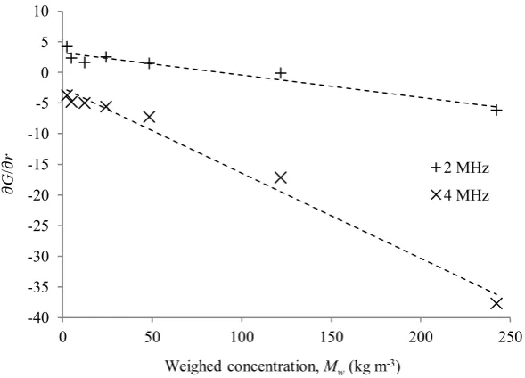
Figure 6: Gradient of G with respect to distance from probe vs. nominal mass concentration, Mw, of Honite 22 (smaller glass) in stirred mixing vessel at ultrasonic frequencies of f = 2 and 4 MHz. Goodness of fit for 2 and 4 MHz data was R2 _{= 0.932 and 0.983, respectively.}

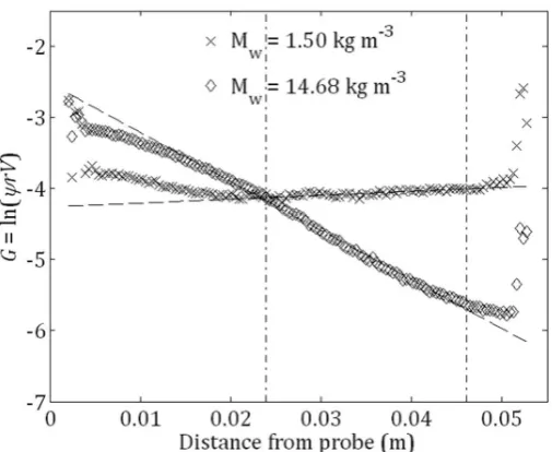
Figure 7 and Figure 8 show the same results, but for the smaller plastic species (Guyblast

40/60). Similar trends are observed as for the glass particles, with a clear linear

dependence of

G

on distance from probe,

r

, and in turn a clear linear dependence of

g

G

/

g

r

on particle concentration. Collectively, these observations demonstrate two things: firstly,

the success of the method as described, and secondly, that the suspensions in the stirred

mixing vessel were, indeed, homogeneous (as linearity would not be expected in

non-homogeneous suspensions, as described in Section II.C). Indeed, this method could be used

as a simple test for homogeneity for a range solid-liquid suspensions in which such

conditions are to be maintained. However, it should be noted that

g

G

/

g

r

could be

calculated over a much smaller range of mass concentrations for the Guyblast plastic

species than for the two Honite glass species. As is clear from Table II, in which the results

0 50 100 150 200 250

g

G

/

g

r

Weighed concentration, Mw(kg m-3)

for

ξh

are summarized, this difference can be accounted for by the fact that attenuation due

to the plastic particles is much higher than for the glass, as would be expected, since the

plastic particles are much larger.

Figure 7: G vs. distance from 4 MHz probe with Guyblast 40/60 (smaller plastic) at two nominal concentrations, Mw = 1.50 and 14.7 kg m-3 in stirred mixing vessel. Dashed lines through data are linear fits. Dot-dashed vertical lines indicate region over which gradients were calculated (r ≈ 24 to 46 mm).

Overall, then, the measured values of the attenuation coefficient,

ξh

, agree well with the

predicted values, especially if the differences in material properties of the particle species

are considered. The main conclusion to be drawn is that the degree of attenuation due to

particles in the suspensions used, as quantified by the gradient of

g

G

/

g

r

, did indeed vary

linearly with particle concentration, as was expected and as has been found by many other

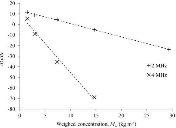
Figure 8: Gradient of G with respect to distance from probe vs. nominal mass concentration, Mw, of Guyblast 40/60 (smaller plastic) in stirred mixing vessel at ultrasonic frequencies of f = 2 and 4 MHz. Goodness of fit for 2 and 4 MHz data was R2 _{= 0.999 and 0.985, respectively.}

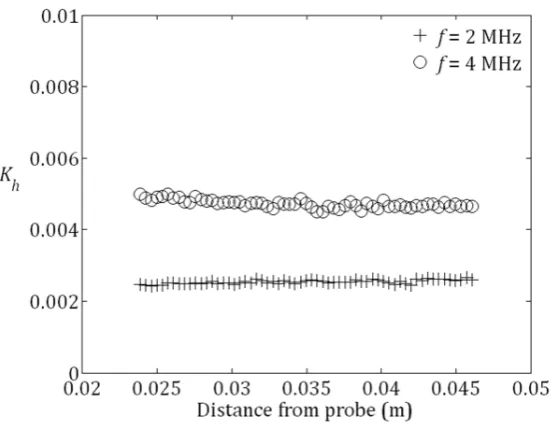
The combined backscatter and system constant in the homogeneous case,

Kh

, was

calculated according to Equation [15] once the corresponding values of

ξh

were known,

from the same runs. In every case, the mean values of

Kh

were calculated over the region

r

≈

24 to 46 mm in order to be consistent with the method of calculation of

ξh

. As a

representative example and for illustration of the degree of variation with distance, Figure

9 shows

Kh

vs

. distance with both the 2 and 4 MHz probes for Honite 22 (smaller glass) at

an intermediate concentration (

Mw

= 12.2 kg m

_{). Relative standard deviations are given in}

the caption. For conciseness, only data at one concentration are shown, but the data at

other concentrations were equally good. The distance-averaged mean values of

Kh

for

Honite 22 (smaller glass) are shown in Figure 10 for both the 2 and 4 MHz probes. The

0 5 10 15 20 25 30

g

G

/

g

r

Weighed concentration, M_w(kg m-3₎

equivalent results for Guyblast 40/60 (smaller plastic) are given in Figure 11 and Figure

12.

Figure 9: Variation of combined backscatter and system constant, Kh, with distance from probe at Mw = 12.2 kg m-3 for smaller glass spheres (Honite 22) at ultrasonic frequencies of f = 2 and 4 MHz in stirred mixing vessel. Relative standard deviation, σ/μ = 2.2 and 2.4 %.

Concentration- and distance-averaged mean values of

Kh

for all particle species and both

ultrasonic frequencies are summarized for all particle species in Table II for reference,

along with predicted values of

ξ

, which were calculated

via

Equations [6] and [10], in which

the measured values of the particle density and size were used (see Table I),

i.e. a

=

d

/2

and

⟨

χ

⟩

=

χ

(

2

=

ka

). (It was not possible to perform a similar comparison for

Kh

, as it

contains a system constant,

kt

, that could not be separated from the backscatter constant,

ksh

, both being incorporated into

Kh

. Measuring

kt

directly would require a more detailed

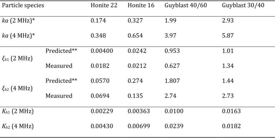
TABLE II: Comparison of predicted and measured values of sediment attenuation constant, ξh, and combined backscatter and system constant, Kh. Values of ka are also given. (All results are given to three significant figures.)

Particle species Honite 22 Honite 16 Guyblast 40/60 Guyblast 30/40

ka (2 MHz)* 0.174 0.327 1.99 2.93

ka (4 MHz)* 0.348 0.654 3.97 5.87

ξh1 (2 MHz)

Predicted** 0.00400 0.0242 0.953 1.01

Measured 0.0182 0.0212 0.627 1.34

ξh2 (4 MHz)

Predicted** 0.0570 0.274 1.807 1.44

Measured 0.0694 0.135 2.74 2.73

Kh1 (2 MHz) 0.00229 0.00363 0.0100 0.0163 Kh2 (4 MHz) 0.00430 0.00699 0.0239 0.0182 * Value based on mean particle diameter, i.e. with a = d50/2.

** Calculated using Equations [6] and [10] by setting a = d50/2 and ⟨χ⟩ = χ(2 = ka).

Several of the expected trends in

Kh

were observed:

Kh

was found to be very constant with

distance (the maximum spatial variation, as quantified by the relative standard deviation,

μ

/

σ

, was 9.4 % for Guyblast 40/60 plastic at

f

= 2 MHz: see Figure 11); and the

distance-averaged values of

Kh

increased with both particle size and ultrasonic frequency (except for

the two Guyblast plastic species at

f

= 4 MHz). However, for all particle species,

Kh

was

found to vary with particle concentration, a result that was not expected, although the

variation for the two Guyblast plastic species was less severe than for the two Honite glass

most probable cause is inaccuracies in

ξh

being propagated into

Kh

through Equation [15]:

when calculated in this way,

Kh

is a strong (indeed, exponential) function of

ξh

. At higher

values of

ka

, multiple scattering is likely to enhance attenuation, and therefore

ξh

and

Kh

, at

higher concentrations, as is observed for Guyblast 40/60 (smaller plastic) at

f

= 2 MHz, for

example (Figure 12). At lower values of

ka

, it may be that absorption becomes a significant

contributor to attenuation, thereby enhancing

Kh

at lower concentrations, as was observed

with Honite 22, the smaller glass species (Figure 11) and as has been noted by Dukhin and

Goetz (2002) in some particle types. Another possibility is that the calculated values of

ξh

and

Kh

were adversely affected by the fact that data were taken at logarithmic, rather than

linear, intervals in the weighed concentration,

Mw

, thus giving undue weight to values at

lower concentrations.

Figure 10: Distance-averaged mean of combined backscatter and system constant, Kh, vs. nominal mass concentration, Mw, for smaller glass spheres (Honite 22) at ultrasonic frequencies of f = 2 and

0 0.002 0.004 0.006

0 50 100 150 200 250

K_h

M

w(kg m-3)

2 MHz

4 MHz in stirred mixing vessel.

Figure 11: Variation of combined backscatter and system constant, Kh, with distance from probe at Mw = 7.38 kg m-3 for smaller plastic particles (Guyblast 40/60) at ultrasonic frequencies of f = 2 and 4 MHz in stirred mixing vessel. Relative standard deviation, σ/μ = 9.4 and 4.4 %.

It is clear from Table II that the measured values of

ξh

are all within a factor of order unity

of the predicted values. More generally, the measured values of both

ξh

and

Kh

increase

with

ka

, as expected: in general,

ξ

and

K

are expected to be proportional to (

ka

)

_{and (}

_ka

₎

_,

respectively, at low

ka

(

i.e.

ka

≪ 1) and approach constant values at high

ka

(

i.e.

ka

> 1),

where

k

is the ultrasonic wavenumber (

k

= 2π/

λ

) and

a

is the particle diameter (Thorne

and Hanes, 2002). However, the discrepancies between the measured and predicted values

of

ξh

are not insignificant, although this conclusion is likely less to be a failure of the

mathematical and measurement techniques developed here, but to be due to the potential

(

i.e.

d

) of measured size distributions (Moate and Thorne, 2013; Thorne and Meral, 2008),

and more generally due to the width of the particle size distributions.

Figure 12: Distance-averaged mean of combined backscatter and system constant, Kh, vs. nominal mass concentration, Mw, for smaller plastic particles (Guyblast 40/60) at ultrasonic frequencies of f = 2 and 4 MHz in stirred mixing vessel.

Factors other than the particle size distribution are present, in particular: differences in

density, compressibility and particle shape between the two spherical glass species

(Honite) and the two non-spherical plastic species (Guyblast) and quartz sand data of

Thorne and Meral (2008) that were used to predict

ξ

. Density is accounted for explicitly in

the model, through Equations [5] and [6], and it is interesting to note that the density

contrast between the fluid and solid phases influences the strength of visco-inertial

scattering (Povey, 1997).

0 10 20 30

K_h

M_{w(kg m}-3₎

2 MHz

However, the influence of the remaining three factors – particle size distribution, particle

shape and compressibility – is not accounted for explicitly in the model and is discussed

below, in that order. First, the effect of width of the particle size distribution is assessed.

Although not accounted for explicitly in the model, the size distribution is incorporated

implicitly through Equations [9] and [10], which were determined empirically. In the

Rayleigh regime (low

ka

),

⟨

χ

⟩

/

χ

> 1,

i.e.

χ

is underestimated; in the geometric regime (high

ka

),

⟨

χ

⟩

/

χ

< 1,

i.e.

χ

is overestimated; in addition, the discrepancy between predicted and

measured values is larger for low

ka

and is proportional to the width of the particle size

distribution, as quantified by

κ

=

σ

/

⟨

a

⟩

(Thorne and Meral, 2008), where

⟨

a

⟩

and

σ

are the

mean and standard deviation of the particle size distribution, respectively. Therefore,

measurements of

ξ

(which is related to

χ

through Equation [6]) will be most sensitive to the

width of the particle size distribution in the case of small, polydisperse species insonified at

low frequencies. This trend is indeed observed in the results presented here: the measured

values of

ξ

(

i.e. ξh

) at lower

ka

are generally lower than those predicted, and higher than

predicted at higher

ka

(see Table II), with the exception of Honite 22, the smaller glass

species, at both ultrasonic frequencies. However, it is stressed that the accuracy of

predicted values of

ξ

depends strongly on the polydispersity of the suspensions, which

varies between species, as can be seen from Figure 1 (Honite glass) and Figure 2 (Guyblast

plastic).

Second, particle shape is likely to have an effect on scattering and attenuation, and both the

plastic species used here are highly non-spherical. According to Thorne and Buckingham

similar volume to a sphere, would have a larger surface area and hence a higher geometric

and scattering cross section”, and it is reasonable to assume that the backscattering and

attenuation properties of highly irregular particles – that is, their ability to absorb and

scatter energy – would be enhanced for the same reasons, since such particles present a

larger projected surface area to the emitted acoustic beam than do spherical particles with

the same volume. However, whether this enhancement of attenuation properties can fully

account for the difference between the observed and predicted values at higher values of

ka

is left as a subject for further study.

Third, the compressibility of the particle species will inevitably affect their scattering and

absorption properties. The strength of thermo-elastic scattering, which influences the

strength of both backscattering and attenuation, is affected by the compressibility contrast

between the liquid and solid phases (Povey, 1997) it is reasonable to conclude that this

contrast is greater for suspensions of Honite glass particles than for Guyblast plastic

particles, suggesting that compressibility is unlikely to be responsible for the differences

between the measured and predicted values of the acoustic coefficients.

To summarize, the discrepancy between the measured and estimated values of

ξ

(and, for

analogous reasons,

K

) can be accounted by a combination of the following: differences in

the physical properties of quartz sand and the species used in this study; and inaccuracies

in the predicted values themselves, which are estimates based on the mean particle size,

rather than entire size distributions. However, overall, the measured values of

ξh

and

Kh

only exist for quartz sand, and so one objective of this study – which was achieved – was to

provide data for other kinds of particle species, in particular highly spherical glass (

i.e.

Honite) and highly non-spherical plastic (Guyblast). The ultimate aim, however, is to use

the measured values of

ξh

and

Kh

to calculate concentration profiles in suspensions in

arbitrary flow geometries of engineering interest

via

a dual-frequency inversion method

(Hurther

et al.

, 2011), as described in the following section.

B.

Implementation of the dual-frequency inversion method with measured acoustic

coefficients in settling suspensions in horizontal pipe flow

To demonstrate the efficacy of the given method for the determination of the acoustic

coefficients

Kh

and

ξh

, a series of measurements were completed in the pipe-flow loop to

observe the settling behavior of flowing suspensions. By using the measured backscatter

voltage, the parameter

J

(

r

) was calculated for a particular distance

r

using Equation [19]

and Φ

₍

_r

_{) using Equation [18] according to the dual-frequency inversion method described}

in Section II.D. The particle concentration,

M

(

r

), through a vertical, wall-normal

cross-section of the pipe could then be evaluated for a particular distance using Equation [23]

(where

ξ

and

ξ

are taken to be the measured values of

ξ

at 2 and 4 MHz,

i.e.

ξh

and

ξh

,

respectively, as given for each particle type in Table II). Some calculated concentration

profiles for the large plastic and the large glass particle species are given in Figure 13 and

Figure 14, respectively, for three different flow rates (

Q

≈ 0.8 to 3.5 l s

_{) and at different}

nominal bulk particle concentrations (

Mw

= 1.50 kg m

_,

d

_{= 0.1 % for plastic;}

_Mw

_{= 24.7 kg}

Figure 13: Concentration by mass, M, vs. reduced distance from centerline, y’/D, at three flow rates:

Q = 3.46, 1.71 and 0.836 l s-1 _{and Ms = 2.15, 1.14 and 0.553 kg m}-3_{, respectively. Larger plastic} particles (Guyblast 30/40 plastic, d50 = 691 μm), nominal mass concentration, Mw = 1.50 kg m-3 (nominal volume fraction, dw = 0.1 %). Note that axes are inverted to aid visualization.

The three flow rates shown in Figure 13 and Figure 14 were chosen because they broadly

correspond to three flow regimes: pseudo-homogeneous, heterogeneous and flow with a

moving and/or stationary bed. It is clear from both sets of concentration profiles presented

in Figure 13 and Figure 14 that at the highest flow rates (

Q

≈ 3.5 l s

_{), the concentration}

gradient is closest to the nominal value through the pipe cross-section, although there is

some variation with depth. Such a pseudo-homogeneous (rather than strictly

homogeneous) flow is characteristic of a suspension in which the upward turbulent

motions of the fluid are greater than the downward gravitational force on the solid

particles. This competition is often quantified by the Rouse number, Ro, such that

0 1 2 3 4 5

-0.5 -0.4 -0.3 -0.2 -0.1 0 0.1 0.2 0.3 0.4 0.5

y

'/

D

Ro = j/k l

_,

_[24]

where

w

is the particle settling velocity, which depends on the particle size, shape and

density,

β

and

k

are constants such that

β

≈ 1 and

k

≈ 0.4, and

u

* is the shear velocity (Allen,

1997). A low Rouse number signifies a fully suspended, well mixed suspension, whereas a

high Rouse number signifies a settling suspension with a strong concentration profile.

Figure 14: Concentration by mass, M, vs. reduced distance from centerline, y’/D, at three flow rates

Q = 3.50, 1.73 and 0.850 l s-1 _{and Ms = 26.6, 20.9 and 10.9 kg m}-3_{, respectively. Larger glass particles} (Honite 16 glass, d50 = 77.0 μm), nominal mass concentration, Mw = 24.7 kg m-3 (nominal volume fraction, dw = 1 %). Note that axes are inverted to aid visualization.

However, at lower flow rates,

M

was found to increase more strongly with distance from

the upper pipe wall,

y

– as would be expected for a real suspension of particles in which the

0 10 20 30 40 50

-0.5 -0.4 -0.3 -0.2 -0.1 0 0.1 0.2 0.3 0.4 0.5

y

'/

D