This is a repository copy of Mixed integer predictive control and shortest path
reformulation.
White Rose Research Online URL for this paper:
http://eprints.whiterose.ac.uk/89731/
Version: Submitted Version
Article:
Bauso, D. (2010) Mixed integer predictive control and shortest path reformulation.
(Unpublished)
[email protected] https://eprints.whiterose.ac.uk/ Reuse
Unless indicated otherwise, fulltext items are protected by copyright with all rights reserved. The copyright exception in section 29 of the Copyright, Designs and Patents Act 1988 allows the making of a single copy solely for the purpose of non-commercial research or private study within the limits of fair dealing. The publisher or other rights-holder may allow further reproduction and re-use of this version - refer to the White Rose Research Online record for this item. Where records identify the publisher as the copyright holder, users can verify any specific terms of use on the publisher’s website.
Takedown
If you consider content in White Rose Research Online to be in breach of UK law, please notify us by
arXiv:1003.2889v1 [math.OC] 15 Mar 2010
Mixed integer predictive control and shortest path reformulation
Dario Bauso
∗March 16, 2010
Abstract
Mixed integer predictive control deals with optimizing integer and real control variables over a receding horizon. The mixed integer nature of controls might be a cause of intractability for instances of larger dimensions. To tackle this little issue, we propose a decomposition method which turns the originaln
-dimensional problem intonindipendent scalar problems of lot sizing form. Each scalar problem is then
reformulated as a shortest path one and solved through linear programming over a receding horizon. This last reformulation step mirrors a standard procedure in mixed integer programming. The approximation introduced by the decomposition can be lowered if we operate in accordance with the predictive control technique: i) optimize controls over the horizon ii) apply the first control iii) provide measurement updates of other states and repeat the procedure.
1
Introduction
1Mixed integer predictive control arises when optimizing integer and real control variables in a receding
2
horizon context [1]. For this reason, many authors see it as a specific field in the broader area of optimal
3
hybrid control [3]. Optimal integer control problems have been receiving a growing attention and are often
4
categorized under different names. See, for instance, the literature on finite alphabet control [5, 9]. Integer
5
control requires a bit more than standard convex optimization techniques. From the literature we know
6
that new properties come into play. As an example, look at multimodularity presented as the counterpart
7
of convexity in discrete action spaces [4]. When talking about mixed integer variables, it is, of course, not
8
possible not to mention the more than vast literature on mixed integer programming [7]. It is exactly in this
9
context that we have found inspiration as clarified in more details next.
10
In this paper, we have moved our steps along the line of [8] which surveys solution methods for mixed
11
integer lot sizing models. Indeed, decomposing ann-dimensional dynamic system intonindipendent lot sizing
12
systems is almost all about this paper is centered around. The approximation introduced by the decomposition
13
can be reduced if we operate in accordance with the predictive control technique: i) optimize controls for
14
each indipendent system all over a prediction horizon, ii) apply the first control to each indipendent system,
15
iii) provide measurement updates of other states and repeat the procedure. The main contribution of this
16
work is to reformulate the mixed integer problem of point i) as a shortest path problem and solve this last
17
through linear programming. This approach mirrors the method surveyed in [8] with the differences that here
18
the shortest path problems run iteratively forward in time over a receding horizon. Reframing the method
19
in a receding horizon context is an element of novelty and presents some additional and new issues which are
20
discussed and overcome throughout the paper.
21
∗Dipartimento di Ingegneria Informatica, Universit`a di Palermo, V.le delle Scienze, 90128 Palermo, ITALY
This paper differs from [1] as we focus on a smaller class of problems that can be solved exactly and do
22
not require advanced relaxation methods which, in turn, are a main topic in [1]. To bring our discussion
23
back to hybrid control, the lot sizing like model used here has much to do with the inventory example briefly
24
mentioned in [3]. There, the authors simply include the example in the large list of hybrid optimal control
25
problems but do not address the issue of how to fit general methods to this specific problem. On the contrary,
26
this work cannot emphasize enough the computational benefits deriving from the “nice structure” of the lot
27
sizing constraints matrix. Binary variables, used to model impulses, match linear programming in a previous
28
work of the same author [2]. There, the linear reformulation is a straightforward derivation of the (inverse) 29
dwell time conditions appeared first in [6]. Analogies with [2] are, for instance, the use of total unimodularity
30
to prove the exactness of the linear programming reformulation. Differences are in the procedure itself upon
31
which the linear program is built up. The shortest path model is an additional element which distinguishes
32
the present approach from [2].
33
This paper is organized as follows. We state the problem in Section 2. We then move to present the
34
decomposition method in Section 3. In Section 4, we turn to introducing the shortest path reformulation and
35
the linear program. We dedicate the last Section 5 to support our theoretical analysis with some numerical
36
results.
37
2
Mixed integer predictive control
38In mixed integer control we usually have continuous state x(k) ∈ Rn, continuous controls u(k) ∈ Rn and disturbancesw(k) ∈Rn, discrete controlsy(k)∈ {0,1}n (see e.g., [1]). Evolution of the state over a finite horizon of lengthN is described by a linear discrete time dynamics in the general form (1), whereA andE
are matrices of compatible dimensions:
x(k+ 1) =Ax(k) +Ew(k) +u(k)≥0, x(0) =x(N) = 0. (1) The above dynamics is characterized by one discrete and continuous control variable per each state, and this
39
reflects the idea that we may wish to control indipendently each state component. Also, starting from initial
40
state at zero, we wish to drive the final state to zero which is a typical requirement when controlling a system
41
over a finite horizon. On this purpose, we have added equality constraints on the final states. Also, we force
42
the states to remain confined within a desired region, take for it the positive orthant, which may describe a
43
safety region in engineering applications or the desire of preventing shortcomings in inventory applications.
44
Continuous and discrete controls are linked together by general capacity constraints (2), where the pa-rameterCis an upper bound on control:
0≤u(k)≤Cy(k), y(k)∈ {0,1}n. (2) For clarity reasons,y(k) is the decision of controlling or not the system, andu(k) is the control action. So if
45
we decide not to control the system then the control action is null, otherwise this last is any value between
46
zero and its upper boundC.
47
The following assumption helps us to describe the common situation where the disturbance seeks to push
48
the state out of the desired region.
49
Assumption 1 (Unstabilizing disturbance effects)
Ew(k)<0. (3)
At this point, the non negative nature of controls u(k) should become much clearer. Actually, control
50
actions are used to push the state far from boundaries into the positive orthant thus to counterbalance the
unstabilizing effects of disturbances over a certain period to come. However, controlling the system has a
52
cost and “over acting” on it is punished by introducing a cost/objective function as explained next.
53
The objective function to minimize with respect to y(k) andu(k) is a linear one including proportional, holding and fixed cost terms expressed by parameterspk,hk, andfk respectively:
N−1 X
k=0
pku(k) +hkx(k) +fky(k)
. (4)
Conditions (1)-(4) introduced so far describe coincisely the problem of interest. In the next section, we
54
recall a standard method to convert the problem of interest (1)-(4) into a mixed integer linear program
55
returning the exact solution in terms of optimal control actionsu(k) andy(k).
56
Remark 1 For sake of simplicity disturbances w(k) are deterministic and apriori known. The approach 57
presented below is still valid if we drop this assumption and turn to consider unknown disturbances. Only, we 58
should carefully repropose problem (1)-(4) in a receding horizon form with iterative measuments updates and 59
control optimization forward in time all over the horizon. 60
2.1
Mixed integer linear program and exact solution.
61
The mixed integer nature of the above program makes it intractable for increasing number of variables and
62
horizon length. So, the topic presented below is motivated mainly by comparisons reasons and applies only
63
to problems of relatively small dimensions.
64
Before introducing the mixed integer linear program we need to define the following notation. Let us start by collecting states, continuous and discrete controls, proportional, holding and fixed costs all in opportune vectors as shown below:
x= [x(0)T. . . x(N)T]T, u= [u(0)T. . . u(N−1)T]T, y= [y(0)T. . . y(N−1)T]T,
p= [(p0)T. . .(pN−1)T]T, h= [(h0)T. . .(hN−1)T]T, f = [(f0)T. . .(fN−1)T]T.
Furthermore, to put dynamics (1) into “constraints” form, let us introduce matrices A, B and vector b
defined as
A=
−I 0 0 . . . 0 0
A −I 0 . . . 0 0 0 A −I . . . 0 0 0 0 A . . . 0 0
..
. ... ... . .. ... ... 0 0 0 . . . A −I
0 0 0 . . . 0 −I
; B=
0 0 . . . 0
B 0 . . . 0 0 B . . . 0 ..
. ... . .. ... 0 0 . . . B
0 0 . . . 0
; b=h−ξ0T (Ew(0))
T
. . .(Ew(N))T −ξTfiT.
Notice that once we take forξ0 andξf the value zero, the first and last rows in the aforementioned matrices
65
restate the constraints on initial and final state of (1).
66
Finally, we are in the condition to establish that problem (1)-(4) can be solved exactly through the following mixed integer linear program:
(M IP C) min
u,y J(u, y) =pu+hx+f y (5)
Ax+Bu=b (6)
The mixed integer linear program (5)-(7) is the most natural mathematical programming representation
67
of the problem of interest (1)-(4). For this reason, throughout this paper we will almost always refer to (5)-(7)
68
when we wish to bring back the discussion to the source problem (1)-(4) and its exact solution.
69
To overcome the intractability of the mixed integer linear program (5)-(7), we propose a new method
70
whose underlying idea is to bring back dynamics (1) to the lot sizing model [8]. To do this, we introduce
71
some additional assumptions on the structure of matrix A which simplify the tractability and affect in no
72
way the generality of the results. This argument is dealt with in details in the next section.
73
2.2
Introducing some structure on
A
74
Our main goal in this section is to rewrite (1) in a “nice” form. With “nice form” we mean a form that
75
emphasizes the analogies with standard lot sizing models [8]. “Stop beating around the bush”, we will
76
henceforth refer to the following dynamics in state of (1):
77
x(k+ 1) =x(k) + ∆x(k) +Ew(k) +u(k)≥0. (8) The reasons why expression (8) is a nice one is that it isolates the dependence of one component state on
78
the other ones. To tell it differently we have separated the influence of all other states on statei. It will be
79
soon clearer that turning our attention to the new expression (8) is a prelude in view of the decomposition
80
approach discussed later on.
81
Once clarified the reasons, we need next to clarify how to go from (1) to (8) and what is the underlying
82
assumption that allows us to do that. Before doing this let us denote withI∈Rn×nthe identity matrix and
83
aij the dependence of state ion statej. So, we can make the following assumption.
84
Assumption 2 MatrixA can be decomposed as
A=I+ ∆, ∆ =
0 a12 . . . a1,n−1 a1n
a21 0 . . . a2,n−1 a2n ..
. ... . .. ... ...
an1 an2 . . . an,n−1 0
.
The reader may notice that (8) is a straighforward derivation of (1) once we take for good Assumption 2.
85
Our secondary goal in this section is to preserve the nature of the game which has stabilizing control
86
actions playing against unstabilizing disturbances. To do this, in our next assumption we do consider the
87
case where the influence of other states on state i is relatively “weak” in comparison to the unstabilizing
88
effects of disturbances.
89
Assumption 3 (Weakly coupling)
∆x(k) +Ew(k)<0. (9)
Notice that the above assumption preserves the nature of the game by bounding the effects of mutual
90
dependence of state components represented by the term ∆x(k). A closer look at (3) and (9) sounds like the
91
term ∆x(k) do not counterbalance the effects ofEw(k). States mutual dependence only emphasize or reduce
92
“weakly” the unstabilizing effects of disturbances.
93
We end this section by noticing that (8) is not yet in “lot sizing” form [8]. In the next section, we present
94
a decomposition approach that translate dynamics (8) into nscalar dynamics in “lot sizing” form [8].
3
Robust decomposition
96With the term “decomposition” we mean a mathematical manipulation through which the original dynamics
97
(8) is replaced bynindependent dynamics of the form:
98
xi(k+ 1) =xi(k)−di(k) +ui(k). (10) The above dynamics is in a typical lot sizing form in the sense that the (inventory) state tomorrowxi(k+ 1)
99
is equal to the (inventory) state today xi(k) plus the discrepancy between today demanddi(k) and today
100
reordered quantityui(k). Changing (8) with (10) is possible once we relate the demanddi(k) to the current
101
values of all other state components and disturbances as expressed below:
102
di(k) = −
h Pn
j=1, j6=iAijxj(k) +
Pn
j=1Eijwj(k) i
= −[∆i•x(k) +Ei•w(k)].
(11)
To tell it differently, we do assume that the influence that all other states have on stateienters into equation
103
(10) through demand di(k) defined in (11). Our next step is to make the n dynamics in the form (10)
104
mutually independent. This is possible by replacing the current state valuesxj(k),j6=iwith their estimated
105
values on the part of agent i which we denote by ˜xj(k),j 6=i. Still with reference to (10), this implies to
106
replace the current demanddi(k) by the “estimated” demand ˜di(k) defined as in (12) whereXk is the set of
107
admissible state vectorsx(k):
108
˜
di(k) = max
ξ∈Xk{−∆i•ξ−Ei•w(k)}. (12)
The idea behind (12) is to take for estimated value the worst admissible demand, i.e., the demand that would push the state out of the positive orthant in a fewest time and such a demand is of course the maximal one. However, it must be noted that we cannot see any drawbacks in combining other decomposition methods with the approach presented in the rest of the paper. To complete the decomposition, it is left to turn the objective function (4) intonindipendent components
Ji(ui, yi) = N−1
X
k=0
pkiui(k) +hkixi(k) +fikyi(k).
Note that because of the linear structure of J(u, y) in (5), it turns J(u, y) = Pn
i=1Ji(ui, yi). So, in the
end we have translated our original problem into nindipendent mixed integer linear minimization problems of the form (13)-(15) as requested at the beginning of this section. In the spirit of predictive control, each minimization problem is then solved forwardly in time all over the horizon. So, forτ = 0, . . . , N−1 we need to solve
(M IP Ci) min ui,yi
N−1 X
k=τ
pkiui(k) +hkixi(k) +fikyi(k)
(13)
xi(k+ 1) =xi(k)−d˜i(k) +ui(k)≥0, xi(τ) =ξi0, xi(N) = 0 (14) 0≤ui(k)≤Cyi(k), yi(k)∈ {0,1}. (15)
It is worth to be noted that non null initial states, which materialize in values ofξ0
i strictly greater than
109
zero in constraints (14) might induce infeasibility of (M IP Ci). So, moving from (M IP C) to (M IP Ci) has
110
this little drawback that we will discuss in more details later on in Section 4.3 together with some other issues
111
concerned with the receding implementation of our method.
112
4
Shortest path and linear programming
113So far, we have first formulated the problem of interest and then decomposed it into nindipendent scalar
114
problems. By the way, decomposition is only the first step of our solution approach. Actually, the mixed
integer nature of variables in (13)-(15) is still an issue to be dealt with. This second part of the work focuses on
116
the relaxation of the integer constraintsyi(k)∈ {0,1}which would facilitate the tractability of the problem.
117
It is well known that relaxation introduces, in general, some approximation in the solution. The main result
118
of this work establishes that, for the problem at hand, relaxing and massaging the problem in a certain
119
manner, will lead to a shortest path reformulation of the original problem. This is a great result as, it is
120
well known that shortest path problem are in turn easily tractable and solvable through linear programming.
121
Shortest path formulations are based on the notion of regeneration interval discussed in details in the next
122
section.
123
4.1
Regeneration interval
[
α, β
]
124
Let us start by introducing a formal definition ofregeneration interval which represents the central topic in
125
this section. The definition, available in the literature for scalar lot sizing models, is borrowed from [8] and
126
adapted to each single (scalar) dynamics i of our decomposedn-dimensional model. So, with reference to
127
the generic minimization problemiexpressed by (13)-(15), let us state what follows.
128
Definition 1 (Pochet and Wolsey 1993) A pair of periods[α, β]form aregeneration intervalfor(xi, ui, yi)
129
ifxi(α−1) =xi(β) = 0 andxi(k)>0 for k=α, α+ 1, . . . , β−1.
130
Given a regeneration interval [α, β], we can define the accumulated demand over the interval dαβi , and
131
the residual demandrαβi as
132
dαβi = β
X
k=α ˜
di(k), rαβi =d αβ i −
$
dαβi C
%
C. (16)
Our idea is now to translate problem (13)-(15) into new variables. More formally, let us consider variables
133
yiαβ(k) andǫαβi (k) defined in (17) with the following meaning. Variableyαβi (k) is equal to one in presence of
134
a saturated control on timekand zero otherwise. Similarly, variableǫαβi (k) is equal to one in presence of a
135
non saturated control on time kand zero otherwise:
136
yiαβ(k) =
1 ifui(k) =C 0 otherwise. ǫ
αβ i (k) =
1 if 0< ui(k)< C
0 otherwise. (17)
To translate the meaning ofyαβi (k) andǫαβi (k) in a lot sizing context, such variables tell us on which period
137
full or partial batches are ordered.
138
At this point and with in mind the above variable transformation, we can rely on well known results in the lot sizing literature which convert the original mixed integer problem (13)-(15) into a number of linear programs LPiαβ, each one associated to a specific regeneration interval. Regeneration intervals and the associated linear programs are mutually related in a way that gives raise to a shortest path problem, which will be the central topic in the next section. For now, we simply repropose below the linear programming problem associated to a single regeneration interval [α, β]. Denoting byek
i =pki +
PN−1
j=k+1h
j
standard manipulation, the linear program for fixed regeneration interval [α, β] appears as:
LPiαβ min yα,βi ,u
α,β i
β
X
k=α
Ceki +fik
yiαβ(k) + β
X
k=α
rαβeki +fik
ǫαβi (k) (18)
β
X
k=α
yiαβ(k) + β
X
k=α
ǫαβi (k) = &
dαβi C
'
(19)
t
X
k=α
yαβi (k) + t
X
k=α
ǫαβi (k)≥
dαt i
C
, t=α, . . . , β−1 (20)
β
X
k=α
yαβi (k) = &
dαβi −rαβi C
'
(21)
t
X
k=α
yiαβ(k)≥
dαt i −rαti
C
, t=α, . . . , β−1 (22)
yαβi (k), ǫαβi (k)≥0, k=α, . . . , β. (23) The above model is extensively used in the lot sizing context. We can limit ourselves to a pair of comments
139
on the underlying idea of the constraints. So, let us start by focusing on the equality constraints (19) and
140
(21). These constraints tell us that the ordered quantity over the interval has to be equal to the accumulated
141
demand over the same interval. This makes sense as initial and final state of a regeneration interval are null
142
by definition. Let us turn our attention to the inequality constraints (20) and (22). There, we impose that
143
the accumulated demand in any subinterval may not exceed the ordered quantity over the same subinterval.
144
Again, this is due to the condition that states are nonnegative at any period of a regeneration interval.
145
Finally, the objective function (18) is simply a rearrangement of (13) induced by the variable transformation
146
seen above and specialized to the regeneration interval [α, β] rather than on the entire horizon [0, N].
147
We are ready to recall the following “nice property” of (LPiαβ) presented first by Pochet and Wolsey in
148
[8].
149
Theorem 1 (Total unimodularity) The optimal solution of (LPiαβ) is feasible. 150
Proof. The proof is based on the observation that the constraint matrix of (LPiαβ) is a 0−1 matrix. We
151
can reorder the constraints in a certain manner, so that matrix has the consecutive 1’s property on each
152
column and turns to be totally unimodular. It follows that yiα,β andǫα,βi are 0−1 in any extreme solution.
153
154
The above theorem represents a first step in the process of converting the mixed integer problem (M IP Ci)
155
into a linear programming one.
156
4.2
Shortest path
157
In the previous section we have introduced a linear programming problem associated to a specific regeneration
158
interval. In this section, we resort to well known results on lot sizing to come up with a shortest path model
159
which links together the linear programming problems of all possible regeneration intervals. Actually, it must
160
be noted that the solution of (13) -(15) can be expressed as a unique regeneration interval [0, N] or as a list
161
of regeneration intervals.
162
So, let us define variables zαβi ∈ {0,1} which tell us one or zero whenever a regeneration interval [α, β]
163
appears or not in the solution of (13) -(15). The linear programming problem solving (13) -(15) takes on the
164
form below. Forτ = 0, . . . , N−1, solve
(LPi) min yαβi ,u
αβ i ,z
αβ i
N−1 X
α=τ+1
N−1 X
β=α β
X
k=α
"
Ceki +fik
yiαβ(k) + β
X
k=α
rαβeki +fik
ǫαβi (k) #
(24)
N
X
β=τ+1
ziτ+1β= 1 (25)
t−1 X
α=τ+1
zα,ti −1−
N
X
β=t
zitβ = 0 t=τ+ 2, . . . , N, τ+ 1≤α≤β≤N (26)
β
X
k=α
yiαβ(k) + β
X
k=α
ǫαβi (k) = &
dαβi C
'
ziαβ, τ+ 1≤α≤β ≤N (27) t
X
k=α
yαβi (k) + t
X
k=α
ǫαβi (k)≥
dαt i
C
ziαβ, t=α, . . . , β−1, τ+ 1≤α≤β≤N (28)
β
X
k=α
yiαβ(k) = &
dαβi −riαβ C
'
ziαβ τ+ 1≤α≤β ≤N (29)
t
X
k=α
yiαβ(k)≥
dαt i −rαti
C
ziαβ, t=α, . . . , β−1, τ+ 1≤α≤β≤N (30)
yαβi (k), ǫαβi (k), ziαβ≥0, k=α, . . . , β. (31)
Let us spend a couple of words on the meaning of the above linear program. Constraints (27)-(31) should
166
be familiar to the reader as they already appeared in (19)-(23). The only difference is that, now, because of
167
the presence of ziαβ in the right hand term, the constraints referring to a given regeneration interval come
168
into play only if that interval is chosen as part of the solution, that is, whenever ziαβ is set equal to one.
169
Furthermore, a new class of constraints appear in (25)-(26). These constraints are typical of shortest path
170
problems and in this specific case help us to force the variables ziαβ(k) to describe a path from 0 to N.
171
Finally, note that forτ = 0, the linear program (LPi) coincide with the linear program presented by Pochet
172
and Wolsey in [8].
173
At this point, we are in a position to recall the crucial result established in [8].
174
Theorem 2 (Pochet and Wolsey, 1993) The linear program (LPi)solves(M IP Ci).
175
Proof. (Sketch) It turns out that the linear program (LPi) is a shortest path problem on variableszα,βi . Arcs
176
are all associated to a different regeneration interval [α, β] and the respective costs are the optimal values of
177
the objective functions of the corresponding linear programs (LPiα,β). We refer the reader to [8] for further
178
details.
179
4.3
Receding horizon implementation of
(
LP
i)
180we specify thatτ goes from 0 toN−1 and for each value ofτwe obtain a new linear program of type (LPi). After we solve (LPi) for τ = 0, we apply the first control to the system, update initial states according to the last available measurements at timeτ = 1 and move to solve a new (LPi) starting at τ = 1. We repeat this procedure until the end of the horizon,τ =N−1. So, consecutive linear programs are linked together by initial state condition expressed in (14), and which we rewrite below
xi(τ) =ξi0.
At this point, we would restate with emphasis the fact that dealing with non null initial states is a main
181
difference between the linear program (LPi) and the linear program used in the lot sizing literature [8]. To
182
counter this little issue, we need to elaborate more on how to compute the accumulated demand in (16).
183
Actually, take for [τ, t] any interval with x(τ) =ξ0
i > s0. Then, condition (16) needs to be revised as
184
dτ t i = max
( t X
k=τ ˜
di(k)−ξi0,0
)
. (32)
The rational behind the above formula has an immediate interpretation in the lot sizing context. Actually,
185
the effective demand over an interval is the accumulated demand reduced by the inventory stored and initially
186
available at the warehouse. From a computational standpoint, the revised formula (32) has a different effect
187
depending on the cases where the accumulated demand exceeds the initial state or not as discussed next.
188
1. Pβ
k=αd˜i(k)≥ξi0: the mixed linear program (M P Ci) with initial statex(τ) =ξ0i >0 and accumulated
189
demandPβ
k=αd˜i(k) is turned into an (LPi) characterized by null initial statex(α−1) = 0 and effective
190
demand dαβi =Pβ
k=αd˜i(k)−ξ
0
i as in the example below:
191
(M P Ci) β
X
k=α ˜
di(k) = 12, x(τ) =ξi0= 10 =⇒ (LPi) x(α−1) = 0, dαβi = 2;
2. Pβ
k=αd˜i(k)< ξi0: the mixed linear program (M P Ci) with initial statex(τ) =ξ0i >0 and accumulated
192
demand Pβ
k=αd˜i(k) is unfeasible. The solution obtained at previous period τ−1 applies. A second
193
example is shown next:
194
(M P Ci) β
X
k=α ˜
di(k) = 7, x(τ) =ξi0= 10 =⇒ (LPi) unfeasible.
In both cases, the revised formula (32) helps us to generalize the linear program (LPi) to cases where
195
the initial state is non null and this is a crucial point when applying the lot sizing model in a receding
196
horizon form.
197
5
Numerical example
198In this specific example, dynamics (1) takes on the form expressed below. Such a dynamics is particularly
199
significative as it reproduces the typical influence between position and velocity in a sampled second-order
200
system. Initial and final states are null and state values must remain in the positive quadrant all over the
201
horizon. More specifically, denoting byx1the position and x2(k) an opposite in sign velocity, the dynamics 202
appears as:
203
x1(k+ 1)
x2(k+ 1)
=
1 −κ κ 1
x1(k)
x2(k)
−
w1(k)
w2(k)
+
u1(k)
u2(k)
≥0,
x1(0)
x2(0)
=
x1(N)
x2(N)
= 0. (33)
A closer look at the first equation reveals that a greater velocityx2(k) reflects into a faster decrease of position 204
velocityx2(k+1) because of some elastic reaction. In both equations, the non negative disturbanceswi(k)≤0
206
seek to push the states xi(k) out of the positive quadrant in accordance to Assumption 3. Their effect is
207
counterbalanced by positive control actions ui. Notice that matrix A can be decomposed as described
208
in Assumption 2. Also, acting on parameter κ we can easily guarantee the “weakly coupling” condition
209
expressed in Assumption 3.
210
Turning to the capacity constraints (2), for this two-dimensional example, these constraints can be rewrit-ten as:
0≤
u1(k)
u2(k)
≤C
y1(k)
y2(k)
,
y1(k)
y2(k)
∈ {0,1}2
.
It is left to comment on the objective function (4). We consider the case where fixed costs are much more relevant than proportional and holding ones. This materializes in choosing a high value forfk in comparison to values of parameterspk,hk as shown in the next linear objective function:
J(u, y) = N−1
X
k=0
(1nu(k) +1nx(k) +100ny(k)).
This choice makes sense for two reasons. First, all the work is centered around issues deriving from the
211
integer nature ofy(k). So, high values offk emphasize the role of integer variables in the objective function.
212
Second, high fixed costs incentivate solutions with the fewest number of control actions and this facilitate
213
the validation and interpretation of the simulated results.
214
The next step is to decompose dynamics (33) in scalar lot sizing form (14) which we rewrite below:
xi(k+ 1) =xi(k)−d˜i(k) +ui(k).
When it comes to the discussion on how to compute the estimated demand ˜di, a natural choice is to set ˜di as
215
below, where we have denoted by ˜x1(k) (respectively ˜x2(k)) the estimated value of statex1(k) (respectively 216
x2(k)) available to agent 2 (agent 1): 217
˜
d1(k)
˜
d2(k)
=
0 κ
−κ 0
˜
x1(k)
˜
x2(k)
+
w1(k)
w2(k)
. (34)
Now, the question is: which expression should we use to represent the set of admissible state vectors Xk
218
appearing in equation (12)? This question has much to do with another one: how does agent 1 predict ˜x2 219
and the same for agent 2 with respect to state ˜x1? A possible answer is shown next: 220
˜
x1(k+ 1)
˜
x2(k+ 1)
=
˜
x1(k)
˜
x2(k)
+
0
κ¯x1
−
0
w2(k) + 0 C , ˜
x1(0)
˜
x2(0)
=
x1(0)
˜
x2(0)
. (35)
Let us elaborate more on the above equations. Regarding to variable ˜x2(k), this is used in the evolution of 221
˜
d1(k) as in the first equation of (34). Because of the positive contribution of the termκx˜2(k) on ˜d1(k), a 222
conservative approach would suggest to take for ˜x2(k) a possible upper bound of x2(k) and this is exactly 223
the spirit behind the evolution of ˜x2(k) as expressed in the second equation of (35). Here, ¯x1 is an average 224
value forx1. A similar reasoning applies to ˜x1(k), used in the evolution of ˜d2(k) as in the second equation of 225
(34). We now observe a negative contribution of the term−κx˜1(k) on ˜d2(k) and therefore take for ˜x1(k) a 226
possible lower bound ofx1(k) as shown in the first equation of (35). 227
We can now move to show and comment our simulated results. We have carried out two different set
228
of experiments whose parameters are displayed in Table 1. In the line of the weakly coupling assumption
229
(see Assumption 3), we have set κsmall enough and in the range equal from 0.01 to 0.225. Such a range
230
works good as we will see that|κxi| is always less thanwi, which also means ∆x(k) +Ew(k)<0. For sake
231
of simplicity and without loss of generality, capacity C is set to three, disturbances wi are unitary and ¯x1 232
is equal to one. Unitary disturbances facilitate the check out and interpretation of the results as when the
233
accumulated demand over the horizon turns to be very close to the horizon length. The two experiments
234
differ also in the horizon lengthN for the reasons clarified next.
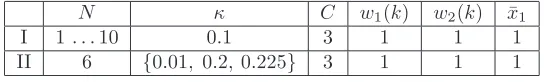
N κ C w1(k) w2(k) x¯1
I 1 . . . 10 0.1 3 1 1 1
[image:12.612.160.432.97.138.2]II 6 {0.01, 0.2, 0.225} 3 1 1 1
Table 1: Simulation parameters chosen for the two experiments.
The first set of experiments aims at analysing the computational benefits of decomposition and relaxation
236
upon which our solution method is based. So, we consider horizon lenghtsN from one to ten. We do not need
237
to consider larger values of N as even in this small range of values, differences in the computational times
238
are already evident enough as clearly illustrated in Fig. 1. Here, we plot the average computational time vs.
239
the horizon lengthN of the mixed integer predictive control problem (solid diamonds), of the decomposed
240
problem (M IP Ci) (dashed squares), and of the linear program (LPi). Average computational time means
241
the average time for one agent to make a single decision (the total time is about 2N times the average one).
242
As the reader may notice, the computational time of the linear program (LPi) is a fraction either of the one
243
requested by the (M P C) or of the one required by the (M IP Ci).
244
(Figure 1 about here)
245
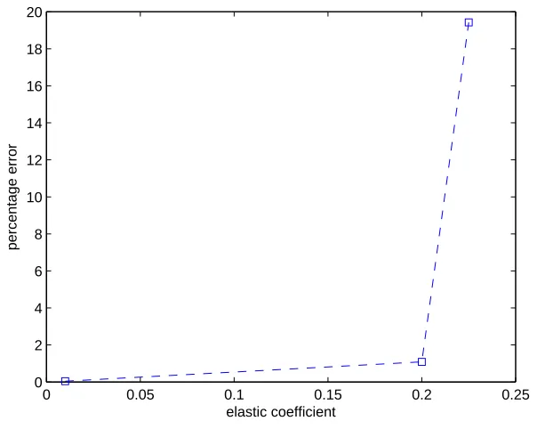
In a second set of simulations, we have inspected how the percentage error
ǫ% = optimal cost of (M P Ci)−optimal cost of (M P C) optimal cost of (M P C) %
varies with different values of the elastic coefficientκ. The role ofκis crucial as we recall thatκdescribes the
246
effective tightness and coupling between different statesx1(k) andx2(k). We do expect that small values for 247
coefficientκ, which means weak coupling of state components, may lead to small errorsǫ%. Differently, high
248
values ofκ, describing a strong coupling between state components, are supposed to induce higher values of
249
ǫ%.
250
This is in line with what we can observe in Fig. 3 where we plot the errorǫ% as function of coefficientκ.
251
For a relatively small values ofκin the range from 0 to 0.2, we observe a percentage error not exceeding the
252
one percent,ǫ%≤1. A discountinuity at aroundκ= 0.2 causes the errorǫ% to go from about 1% to 20%.
253
(Figure 2 about here)
254
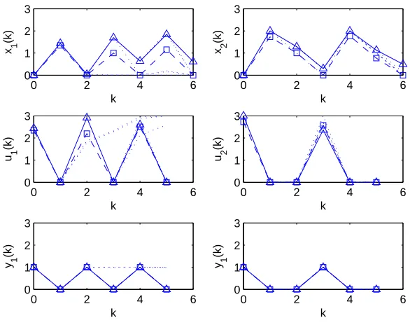
We might not be surprised as discountinuity of errors is typical in mixed integer programs and we try to
255
clarify this in more details in the plot of Fig. 4. Here, for a horizon lengthN = 6 and for a relatively high
256
value ofκ= 0.225, we display the exact solution (dashed squares) and approximate solution (solid triangles)
257
returned by the mixed integer linear program (M IP C) and by the linear program (LPi) respectively. The
258
solution is in terms of the time plot of states xi(k), continuous controlsui(k) and discrete controls yi(k).
259
Dotted lines represent predicted trajectories in earlier periods of the receding horizon implementation. At a
260
first check, and this is in accordance with what we do expect, we note that controlsui(k) never exceed the
261
capacity and are always associated to unitary control actions yi(k). Now, with a look at the behaviour of
262
discrete controlsy1(k), it can be observed that the approximate solution presents four control actions (four 263
peaks at one), whereas the exact solution has control y1(k) acting on the system only three times (three 264
peaks at one). One peak out of four represents an increase in the use of control actions of about 25 percent
265
which reflects into an approximate increase in the percentage error of 20%. A last observation concerning
266
the exact plot ofyi(k) is that the number of control actions are as minimal as possible, i.e., three fory1(k) 267
and two fory2(k). This makes sense as the accumulated demand over the horizon approximates by above the 268
horizon length. This implies that the minimum number of control actions can be roughly obtained dividing
269
the accumulated demand (about something above six) by the capacityC (equal to three) and rounding the
270
fractional result up to the next integer.
(Figure 3 about here)
272
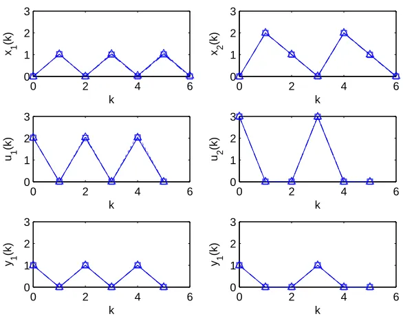
Let us move to compare exact and approximate solutions for a smaller value of κ = 0.2. With reference
273
to Fig. 4, we observe that, differently from above, discrete controlsyi(k) coincide. However, we still have
274
notable differences in the plot of continuous controlsu1(k) which cause distinct state trajectories for x1(k). 275
Small differences can be noted for u2(k) and x2(k) as well. The observed differences still cause a reduced 276
percentage errorǫ% = 1.
277
(Figure 4 about here)
278
We conclude our simulations by showing that the percentage errorǫ% is around zero when we reduce further
279
the value ofκto 0.01. This is evident if we look at Fig. 5, where plots of different styles overlap which means
280
that exact and approximate solutions coincide.
281
(Figure 5 about here)
282
References
283[1] D. Axehill, L. Vandenberghe, and A. Hansson, “Relaxations applicable to mixed integer predictive
284
control Comparisons and efficient computations”, in Proc. of the 46th IEEE Conference on Decision 285
and Control, New Orleans, USA, pp. 4103–4109, 2007.
286
[2] D. Bauso, “Boolean-controlled systems via receding horizon and linear programing”, Mathematics of 287
Control, Signals, and Systems (MCSS), vol. 21, no. 1, 2009, pp. 6991.
288
[3] M. S. Branicky, V. S. Borkar and S. K. Mitter, “A Unified Framework for Hybrid Control: Model and
289
Optimal Control Theory”,IEEE Trans. on Automatic Control, vol. 43, no. 1, 1998, pp. 31–45.
290
[4] P. R. De Waal and J. H. Van Schuppen, “A class of team problems with discrete action spaces: optimality
291
conditions based on multimodularity”,SIAM Journal on Control and Optimization, vol. 38, pp. 875–892,
292
2000.
293
[5] G.C. Goodwin and D.E. Quevedo, “Finite alphabet control and estimation”, International Journal of 294
Control, Automation, and Systems, vol. 1, no. 4, pp. 412–430, 2003.
295
[6] J. Hespanha, D. Liberzon, A. Teel, “Lyapunov Characterizations of Input-to-State Stability for Impulsive
296
Systems”,Automatica, vol. 44, no. 11, 2008, pp. 2735–2744.
297
[7] G. L. Nemhauser, and L. A. Wolsey,Integer and Combinatorial Optimization, John Wiley & Sons Ltd,
298
New York, 1988.
299
[8] Y. Pochet, and L. A. Wolsey, “Lot Sizing with constant batches: Formulations and valid inequalities”,
300
Mathematics of Operations Research, vol. 18, no. 4, pp. 767–785, 1993.
301
[9] D. C. Tarraf, A. Megretski and M. A. Dahleh, “A Framework for Robust Stability of Systems Over
302
Finite Alphabets”,IEEE Transactions on Automatic Control, vol. 53, no. 5, pp. 1133– 1146, June 2008.
0 5 10 15 20 10−2
10−1 100 101 102
N
[image:14.612.144.439.131.370.2]sec
Figure 1: Average computational time vs. horizon lengthN of the mixed integer predictive control problem (solid diamonds), of the decomposed problem (M IP Ci) (dashed squares), and of the linear program (LPi).
0 0.05 0.1 0.15 0.2 0.25
0 2 4 6 8 10 12 14 16 18 20
elastic coefficient
percentage error
[image:14.612.144.446.477.718.2]0 2 4 6 0
1 2 3
x 1
(k)
k
0 2 4 6
0 1 2 3
x 2
(k)
k
0 2 4 6
0 1 2 3
u 1
(k)
k
0 2 4 6
0 1 2 3
u 2
(k)
k
0 2 4 6
0 1 2 3
y 1
(k)
k
0 2 4 6
0 1 2 3
y 1
(k)
[image:15.612.148.439.124.354.2]k
Figure 3: Elastic coefficient κ = 0.225. Exact solution (dashed squares) and approximate solution (solid triangles) returned by the mixed integer linear program (M IP C) and by the linear program (LPi) respectively. Horizon lengthN = 6. Time plot of statesxi(k), continuous controlsui(k) and discrete controlsyi(k).
0 2 4 6
0 1 2 3
x 1
(k)
k
0 2 4 6
0 1 2 3
x 2
(k)
k
0 2 4 6
0 1 2 3
u 1
(k)
k
0 2 4 6
0 1 2 3
u 2
(k)
k
0 2 4 6
0 1 2 3
y 1
(k)
k
0 2 4 6
0 1 2 3
y 1
(k)
k
[image:15.612.146.439.462.694.2]0 2 4 6 0
1 2 3
x 1
(k)
k
0 2 4 6
0 1 2 3
x 2
(k)
k
0 2 4 6
0 1 2 3
u 1
(k)
k
0 2 4 6
0 1 2 3
u 2
(k)
k
0 2 4 6
0 1 2 3
y 1
(k)
k
0 2 4 6
0 1 2 3
y 1
(k)
[image:16.612.146.439.291.524.2]k