This is a repository copy of
Uncertainty Analyses in the Finite-Difference Time-Domain
Method
.
White Rose Research Online URL for this paper:
http://eprints.whiterose.ac.uk/10729/
Article:
Edwards, R.S., Marvin, A.C. orcid.org/0000-0003-2590-5335 and Porter, S.J. (2010)
Uncertainty Analyses in the Finite-Difference Time-Domain Method. IEEE Transactions on
Electromagnetic Compatibility. 5342494. pp. 155-163. ISSN 0018-9375
https://doi.org/10.1109/TEMC.2009.2034645
[email protected] https://eprints.whiterose.ac.uk/ Reuse
Items deposited in White Rose Research Online are protected by copyright, with all rights reserved unless indicated otherwise. They may be downloaded and/or printed for private study, or other acts as permitted by national copyright laws. The publisher or other rights holders may allow further reproduction and re-use of the full text version. This is indicated by the licence information on the White Rose Research Online record for the item.
Takedown
If you consider content in White Rose Research Online to be in breach of UK law, please notify us by
promoting access to White Rose research papers
White Rose Research Online
[email protected]
Universities of Leeds, Sheffield and York
http://eprints.whiterose.ac.uk/
This is an author produced version of a paper published in the journal
IEEE TRANSACTIONS ON ELECTROMAGNETIC COMPATIBILITY
White Rose Research Online URL for this paper:
http://eprints.whiterose.ac.uk/10729
Published paper
Edwards, RS; Marvin, AC; Porter, SJ
(2010)
Uncertainty Analyses in the Finite-Difference Time-Domain Method
IEEE TRANSACTIONS ON ELECTROMAGNETIC COMPATIBILITY
52 (1) 155-163
IEEE TRANSACTIONS ON ELECTROMAGNETIC COMPATIBILITY, VOL. 52, NO. 1, FEBRUARY 2010 155
Uncertainty Analyses in the Finite-Difference
Time-Domain Method
Robert S. Edwards, Andrew C. Marvin
, Senior Member, IEEE
, and Stuart J. Porter
, Member, IEEE
Abstract—Providing estimates of the uncertainty in results ob-tained by Computational Electromagnetic (CEM) simulations is essential when determining the acceptability of the results. The Monte Carlo method (MCM) has been previously used to quan-tify the uncertainty in CEM simulations. Other computationally efficient methods have been investigated more recently, such as the polynomial chaos method (PCM) and the method of moments (MoM). This paper introduces a novel implementation of the PCM and the MoM into the finite-difference time -domain method. The PCM and the MoM are found to be computationally more efficient than the MCM, but can provide poorer estimates of the uncertainty in resonant electromagnetic compatibility data.
Index Terms—Computational electromagnetism, finite-difference time domain (FDTD), method of moments (MoM), Monte Carlo, polynomial chaos, uncertainty analysis.
I. INTRODUCTION
C
OMPUTATIONAL electromagnetic (CEM) simulations rely on sets of input parameters, which often have an as-sociated uncertainty. These uncertainties may arise from a lack of precise knowledge of the material parameters or geometries that are being modeled. Uncertainties in these input parameters lead to uncertainties in the output of the CEM simulations. This type of uncertainty is often known as parameter uncertainty. In this paper, a determination of the parameter uncertainty in the re-sults of finite-difference time-domain (FDTD) simulations will be made. Quantifying the uncertainty in the output of interest amounts to quantifying the standard deviation of the output. Un-certainty analyses provide the quantitative level of confidence that may be held in the results of CEM simulations. This in-formation is essential when determining whether the results are acceptable or useful.Previous research has already highlighted the importance of quantifying uncertainty in CEM [1]–[4]. This research uses the Monte Carlo method (MCM), which is generally accepted as being an accurate uncertainty analysis (UA) method, to test the performance of other computationally efficient UA methods. Chauvi`ere published work involving the implementation of the polynomial chaos method (PCM) into a higher order discontinu-ous Galerkin solution of Maxwell’s equations [1]. The PCM was found to accurately quantify the output uncertainty, while be-ing more computationally efficient than the MCM. Chauvi`ere’s work, however, only estimated the output uncertainty due to one uncertain input parameter. The accuracy and computational
Manuscript received December 17, 2008; revised July 2, 2009. First published December 1, 2009; current version published February 18, 2010.
The authors are with the Department of Electronics, University of York, York, YO10 5DD, U.K. (e-mail: [email protected]).
Digital Object Identifier 10.1109/TEMC.2009.2034645
efficiency of this method with increased numbers of uncertain input parameters needs to be analyzed.
More recently, Ajayi has discussed the use of a direct solu-tion technique (DST) to quantify uncertainty [2]. This technique applies the probabilistic method of moments (MoM) [5], [6] to different CEM schemes, such as the transmission line matrix (TLM) method. Ajayi used the DST to estimate the uncertainty in the frequency of the first resonance for simple electromag-netic problems [2]. The DST was found to work well for small parameter variations, giving results that are in agreement with results obtained from the MCM [2].
This paper outlines novel implementations of the PCM and the MoM into the FDTD method. It is possible to implement these statistical methods into other CEM techniques. The un-certainty in the output of simulations performed using different CEM methods and different levels of accuracy will be of a similar size. However, with the results of different simulations formed by different CEM techniques, the uncertainty in the out-put will have a dependence on the method used and the accuracy with which the simulation is performed. This paper considers only the FDTD method so that a fair analysis of the PCM, the MoM, and the MCM can be formed.
In this paper, the UA methods are used to obtain the un-certainty in the output electric field viewed in the frequency domain. In the first of two examples, the UA methods are used to estimate the uncertainty in the electric field that penetrates a shielded enclosure containing a printed circuit board (PCB), at around 1.8 GHz. This example is fairly simple, having only one uncertain input parameter and encompassing only a few resonant features. The second electrically large example considers three uncertain inputs, encompassing many more resonant modes. The PCM and the MoM are compared to the MCM in terms of their ability to accurately quantify the uncertainty and their com-putational expense. The uncertain input parameters considered in this paper are all assumed to be uncorrelated. When consider-ing correlated variables, United Kconsider-ingdom Accreditation Service (UKAS) [6] suggests grouping all correlated variables into one single grouped variable, which will subsequently be uncorre-lated with all other uncertain variables in the sample.
In this paper, the uncertainty in the output of interest is a fre-quency response curve. The feature selective validation (FSV) method [7], [8] is used in this paper to determine the similarity of the uncertainty curves formed from the different UA meth-ods. This method is a numerical technique, which determines how similar two curves are in terms of their amplitude and fea-ture differences. The amplitude and feafea-ture differences between the curves are combined to give a general difference measure (GDM). This method currently forms part of a draft standard for the verification and validation of CEM models [9].
156 IEEE TRANSACTIONS ON ELECTROMAGNETIC COMPATIBILITY, VOL. 52, NO. 1, FEBRUARY 2010
II. UA METHODS
A. Monte Carlo Method
To determine the uncertainty in an FDTD simulation via the MCM, the probability density functions (PDFs) associated with the uncertain input parameters must first be sampled many times. In this paper, latin hypercube sampling (LHS) [10] is chosen as the preferred sampling method. This has been shown to produce a converged solution more quickly than other sampling methods [10]. The samples, obtained from the PDFs, form sets of input parameter values: one FDTD simulation is performed for each set. The outputs formed from each simulation are combined to form the output mean and standard deviation. The uncertainty in the output is represented by the standard deviation.
It is well known that the MCM has slow convergence, and as such, it is a computationally expensive method. The mean and uncertainty, formed using the MCM, converge for large numbers of samples. Once convergence has been reached, the use of more samples does not change the mean and uncertainty significantly. In this paper, the FSV method is used, in a novel way, to determine when the MCM has reached convergence. The mean and uncertainty formed in this paper are frequency response curves. The FSV method is used to compare the re-spective mean and uncertainty frequency response curves after everyN simulations. Convergence is reached when the mean and uncertainty curves are determined to be “excellent” matches to the respective mean and uncertainty curves produced afterN simulations previously. In the examples in this paper,N = 50
and convergence is reached when the comparisons of the re-spective mean and uncertainty curves produce a GDM<1.5. This novel way of using FSV provides an accurate, consistent, and impartial way of determining convergence, when the output of interest is a curve.
B. Polynomial Chaos Method
The concept of homogeneous chaos was first introduced by Wiener [11]. Homogeneous chaos uses Hermite polynomials to represent stochastic processes that depend on uncertain input parameters, which follow normal distributions [12]. The PCM is a more generalized method for dealing with inputs that are not necessarily normally distributed. In the PCM, certain orthogonal basis polynomials are selected, depending on the distributions of the random input variables [12]. A function depending on the uncertain random variables can be expanded in terms of the selected polynomials. This expansion, which is known as the Wiener–Askey chaotic expansion [12], casts the uncertainty in the output into the orthogonal polynomials alone. The orthogo-nality of the polynomial basis set can reduce stochastic differ-ential equations to a set of deterministic differdiffer-ential equations that can be solved numerically [12].
Xiu and Karniadakis [12] found the PCM to be computa-tionally cheaper than the MCM. However, they noted that the method’s efficiency is problem specific [13].
1) Wiener–Askey Chaos: Any second-order random process X, depending on some random event θ, can be represented
as [12]
X(θ) =
∞
i= 0
ciψi(ζ(θ)) (1)
whereciare constant coefficients and
ζ(θ) = (ζ1(θ), ζ2(θ), . . .) (2)
represents a vector containing an infinite number of indepen-dent random variables [12]. The polynomial basis sets {ψi},
corresponding to the random variablesζ(θ), are chosen from the Askey-scheme, which can be found in [12].
The polynomial basis sets are all orthogonal, which implies that
ψiψj=ψ2iδij (3)
whereδij is the Kronecker delta and the inner product., .is
defined as [12]
f(ζ)g(ζ)=
f(ζ)g(ζ)w(ζ)dζ. (4)
The weighting functionw(ζ)corresponds to the choice of poly-nomial basis{ψj}.
2) General Polynomial Chaos: The Weiner–Askey chaotic expansion (1) can be used to solve stochastic differential equa-tions [12]. Letu(x, t, θ)be a solution of the stochastic differ-ential equation
L(x, t, θ)u(x, t, θ) =f(x, t, θ) (5)
where x,t,andθ represent position, time and some random event, respectively. The symbolLrepresents some differential operator andf is a source term [12]. The solution umay be regarded as a random process and expanded as [12]
u(x, t, θ) =
P
i= 0
ui(x, t)ψi(ζ(θ)). (6)
For practical applications, the infinite sum in (1) has been trun-cated atPhere. Ifdis the order of the highest order polynomial used in the expansion andnis the dimension of the random variableζ, then
P+ 1 = (n+d)!
n!d! . (7)
Substituting the expansion ofuinto (5) yields
L(x, t, θ)
P
i= 0
ui(x, t)ψi(ζ(θ)) =f(x, t, θ). (8)
The inner product of both sides of this equation can be formed withψk to give
L(x, t, θ)
P
i= 0
ui(x, t)ψi(ζ(θ)), ψk
=f(x, t, θ), ψk. (9)
The orthogonality of the basis polynomials reduces (9) to a set of(P+ 1)differential equations: one for eachui [12]. These
equations are deterministic [12] and can, therefore, be solved
EDWARDSet al.: UNCERTAINTY ANALYSES IN THE FDTD METHOD 157
numerically. Once eachui is found, the mean and variance of u(x, t, θ)can be calculated. The mean is calculated as [1]
¯
u(x, t, θ) =u(x, t, θ),1=
P
i= 0
uiψi,1
=
P
i= 0
uiψi, ψ0=
P
i= 0
uiδi0 =u0 (10)
using the fact thatψ0 = 1for all polynomial bases. The variance can be obtained in a similar way by first calculating
u(x, t, θ), u(x, t, θ)=
P
i= 0
P
j= 0
uiujψi, ψj
=
P
i= 0
P
j= 0
uiujδijψi2= P
i= 0
u2iψi2.
(11)
The variance ofu(x, t, θ)is therefore [1]
σ2 =u(x, t, θ), u(x, t, θ) − u(x, t, θ),12
=
P
i= 0 u2
iψi2 −u20 =
P
i= 1 u2
iψ2i. (12)
The uncertainty inu(x, t, θ)is the standard deviationσ. 3) General Polynomial Chaos in FDTD: General polyno-mial chaos has already been successfully applied to computa-tional fluid dynamics (CFD) [14], [15] and specific areas of CEMs [1]. The application of general polynomial chaos to 1-D FDTD is given here, and these arguments can be easily gener-alized to three dimensions.
Maxwell’s equations for a wave propagating in a linear isotropic homogeneous material along thex-axis in 1-D are
∂Hz ∂t =−
1
µ ∂Ey
∂x (13)
∂Ey ∂t =−
1
ǫ
∂Hz ∂x +σEy
. (14)
As usual,Hz(x, t)represents the magnetic field oriented in the z-direction, at a positionxand timet. Similarly,Ey represents
the electric field oriented in they-direction. The symbolsµ,ǫ, andσrepresent the permeability, permittivity, and conductivity of the medium in which the electromagnetic fields propagate. CEM models seek to solve these two coupled equations to find approximations forHz(x, t)andEy(x, t). If there are
uncer-tain input parameters, then the solutions will depend on some random event θ. The uncertain field solutions can, therefore, be represented asHz(x, t, θ)andEy(x, t, θ). The solutions to
Maxwell’s equations may be found by using the FDTD scheme, first proposed by Yee [16].
In Yee’s scheme, the temporal and spatial partial derivatives in Maxwell’s equations are approximated using central difference approximations. The problem space is discretized into cells of length∆x, and the time is split into discrete intervals∆t. This yields two update equations, which form the basis of the 1-D
FDTD solution. The update equations formed are
Hn+ (1/2)
z
j+1 2, θ
=Hn−(1/2)
z
j+1 2, θ
−γ[Eyn(j+ 1, θ)−Eyn(j, θ)] (15)
and
Eyn+ 1(j,θ) =αEyn(j, θ) +β
Hzn+ (1/2)
j−1
2, θ)
−Hn+ (1/2)
z
j+1 2, θ
. (16)
The shorthand notationHn
z(j, θ) =Hz(j∆x, n∆t, θ)is used in
the previous equations, wherejandnare positive integers. The material properties of the medium in which the fields propagate are represented by
α=α(x, θ) = 1−σ(x, θ)∆t/2ǫ(x, θ)
1 +σ(x, θ)∆t/2ǫ(x, θ) (17)
β =β(x, θ) = ∆t
∆xǫ(x, θ)(1 +σ(x, θ)∆t/2ǫ(x, θ) (18)
and
γ=γ(x, θ) = ∆t
∆xµ(x, θ). (19)
The material propertiesµ,ǫ,andσ,all depend on the uncertain parameter θ. This dependence is defined by the PDFs of the input parameters.
The 1-D FDTD update equations defined above are used to obtain solutions for the electric and magnetic fields, subject to some electric field source. The field solutions can be expanded in terms of the appropriate orthogonal polynomials {ψi} to
separate the dependence of the field on the random parameterθ from the dependence on time and position. The field solutions are expanded as
Eyn(j, θ) = P
i= 0
eni(j)ψi(ζ(θ)) (20)
and
Hzn(j, θ) = P
i= 0
hni(j)ψi(ζ(θ)). (21)
The coefficients en
i(j) andhni(j) must be found so that the
mean and uncertainty of the output fields can be formed. The following discussion outlines how to obtain the field coefficients en
i(j)andhni(j).
Expansions (20) and (21) can be substituted into (15) and (16) to obtain
P
i= 0
hni+ (1/2)(j+ 1/2)ψi(ζ(θ)) = P
i= 0
hni−(1/2)(j+ 1/2)
158 IEEE TRANSACTIONS ON ELECTROMAGNETIC COMPATIBILITY, VOL. 52, NO. 1, FEBRUARY 2010
and
P
i= 0
eni+ 1(j)ψi(ζ(θ)) = P
i= 0
αeni(j)ψi(ζ(θ))
+β
hni+ (1/2)(j−1/2)−h n+ (1/2)
i (j+ 1/2)
ψi(ζ(θ)).
(23)
At this point, the electric field source Es may be added into
(23). If this field source has some associated uncertainty, then it may be expanded as
Esn(j, θ) = P
i= 0
eni,s(j)ψi(ζ(θ)). (24)
Adding this source term into (23) yields
P
i= 0
eni+ 1(j)ψi= P
i= 0
αeni(j)ψi+eni,s(j)ψi
+β
hni+ (1/2)(j−1/2)−hni+ (1/2)(j+ 1/2)
ψi. (25)
Taking the inner product of both sides of (22) and (25) with some test polynomial ψk, wherek is an integer in the range
0≤k≤P, reduces the equations to
hnk+ (1/2)(j+ 1/2) =hnk−(1/2)(j+ 1/2)
− 1 ψ2
k P
i= 0
[(eni(j+ 1)−eni(j))γψiψk] (26)
and
enk+ 1(j) =enk ,s+ 1(j) +
1
ψ2
k P
i= 0
eni(j)αψiψk
+
hni+ (1/2)(j−1/2)−h n+ (1/2)
i (j+ 1/2)
βψiψk.
(27)
The previous two equations make use of the orthogonality rela-tion set out in (3). The material propertiesα,β, andγremain in the inner products due to their dependence onθ.
Equations (26) and (27) can be used to calculateen k(j)and hnk+ 1/2(j+ 1/2) for alln andj, andk= 0, . . . , P. In order to do this, the inner productsαψiψk,βψiψk,andγψiψk
must first be calculated for alli, k= 0, . . . , P. These can be cal-culated using numerical integrations as a preprocess; the update equations can then be used in a similar manner to the leapfrog scheme used in conventional FDTD. The source term must also be calculated at each time step as
enk ,s(j) =
1
ψ2
k
Ens(j, θ)ψk(ζ(θ)). (28)
To complete the scheme, update equations are required at the boundary. The examples in this paper consider the scattering of electromagnetic fields in free space, and therefore, the first-order Mur absorbing boundary condition [17] is chosen as a relevant boundary condition. At the lower boundary (wherej= 0), the
usual Mur update equation is
Eyn+ 1(0) =Eyn(1) +
β(1)γ(1)−1
β(1)γ(1) + 1
Eyn+ 1(1)−Eny(0)
.
(29) Introducing uncertainty into this equation via dependence onθ yields
Eyn+ 1(0, θ) =Eyn(1, θ)
+
β(1, θ)γ(1, θ)−1
β(1, θ)γ(1, θ) + 1
Eyn+ 1(1, θ)−Eyn(0, θ)
. (30)
As before, the field terms can be expanded using the chaotic expansion, and an inner product of both sides of the resulting equation can be taken with ψk. Carrying out these two steps
gives
enk+ 1(0) =enk(1) +
1
ψ2
k P
i= 0
eni+ 1(1)−eni(0)
ξ(1, θ)ψiψk
(31)
whereξis defined as
ξ(1, θ) =
β(1, θ)γ(1, θ)−1
β(1, θ)γ(1, θ) + 1. (32)
Usually, at the boundaries, the properties of the medium are those of free space: there is no uncertainty in the parameter values near the boundary. Thus,ξ has no θ dependence and
ξψiψk=ξδikψk2. The update equation for the electric field
at the lower boundary reduces to
enk+ 1(0) =enk(1) +ξ(1)
enk+ 1(1)−enk(0)
(33)
fork= 0, . . . , P. Using a similar argument, the electric field update equation at the upper boundary (j=N) is
enk+ 1(N) =ekn(N−1) +ξ(N−1)
enk+ 1(N−1)−enk(N)
. (34) The coefficientsen
k(j)may now be calculated using (26), (27),
(33), and (34). Similar equations to (10) and (12) are formed for the mean value ofEyn(j, θ)
¯
Ey =en0(j) (35)
and the variance
σ2 =
P
i= 1
(eni(j))2ψ2i. (36)
The PCM is easily applied to FDTD because the update equa-tions follow a very similar form to those in conventional FDTD. The only extra step comes in calculating the integrals that cor-respond to the inner products in the update equations (26) and (27). The application of the PCM to FDTD given here may be easily generalized to 3-D.
One problem with the PCM arises when trying to form the mean and uncertainty of some related quantity, which does not depend linearly onEn
y(j, θ). For example the output of interest
EDWARDSet al.: UNCERTAINTY ANALYSES IN THE FDTD METHOD 159
may be the absolute value ofEyn(j, θ). The meanµof this output
is formed as
µ=|Eny(j, θ)|,1=
P
i= 0
eni(j)ψi(ζ(θ))
ψ0
. (37)
The absolute value within the inner product prevents the or-thogonality of the basis polynomials from being used to form a simple relationship for the mean. The mean will have to be calculated using a numerical integration over the uncertain pa-rameter space θ. This presents a problem with the PCM: the calculation of the mean of the output of interest is not always trivial. Some of the mathematical simplicity of the PCM has been lost by trying to form the mean of the quantity|En
y(j, θ)|.
The mean must be calculated using a numerical integration at each frequency point, which requires extra computational time. This extra computational expense is, however, small compared to the PCM simulation runtime. Once this mean has been cal-culated, the varianceσ2 may be calculated using the standard definition
σ2(|Eyn(j, θ)|) =(|Eyn(j, θ)| −µ)2. (38)
Further numerical integrations are required to obtain this vari-ance. The uncertainty in|En
y(j, θ)| is the square root of this
variance.
The PCM performs one large simulation, storing a factor
(P+ 1) more field coefficients and (P+ 1)2 more material parameter values (via the inner products) than the MoM and the MCM. If there are, for example, three uncertain inputs and the Wiener–Askey chaos expansion is truncated at first order, thenP = 3,and the PCM will require around 16 times more memory than the MoM and the MCM to store the material inner products.
The computational time required by the PCM is somewhat more difficult to analyze. Since there are(P+ 1)field coeffi-cients to solve for and each calculation requires the sum of the product of(P+ 1)field coefficients with(P+ 1)material inner products [see (26) and (27)], the computational time required by the PCM will be approximately(P+ 1)2 greater than that of a single FDTD simulation. In addition to this, extra compu-tational time is required to calculate the material inner products at each point in the problem space and the output variance from the field coefficients. These extra numerical integrations add to the overall computational effort of the PCM; however the com-putational time will scale approximately with(P+ 1)2. This computational time will be greater than that required for the MoM, but should be less than that required for the MCM.
C. Method of Moments
The MoM is another approximate UA method, which is sim-ilar to the method outlined in [6] for the determination of uncer-tainty in practical electromagnetic compatibility (EMC) mea-surements. It is the internationally accepted method outlined in [5] for the propagation of uncertainties through a model.
The MoM uses a first-order Taylor series expansion of the output electric fieldEy about the mean input parameter values
Ey(p1, . . . , pn) =c1p1+· · ·+cnpn (39)
wherecirepresent the sensitivity derivatives of each parameter pievaluated at the mean parameter valuesp¯i. For the purposes
of this discussion, it is assumed that there areninput parameters for the FDTD simulation.
The mean output electric fieldE¯yis calculated by performing
one simulation with all input parameters taking on their mean values [5], [6]. To calculate the sensitivity derivativeci, in (39),
an FDTD simulation must be performed with all parameters taking on their mean values, except for the parameter pi. In
this simulation, the parameterpi is perturbed slightly from its
mean value to givepi= ¯pi+ ∆. This simulation will produce a
perturbed output electric fieldEi
y. The sensitivity derivativeci
is calculated using the finite-difference approximation
ci= Ei
y−E¯y
∆ . (40)
Ifuiis the uncertainty in the parameterpi, determined from the
PDF ofpi, then the uncertainty in the mean output of the FDTD
simulation is calculated as [5], [6]
σ=
n
i= 1 c2iu2i
1/2
. (41)
The accuracy of the uncertainty estimate relies on the relation-ship between the uncertain inputs and the output of interest being linear. The method is also dependent on the size of the perturbation ∆ that is used. It has been previously suggested that using a perturbation∆ =uiis appropriate [5], [6].
The MoM requires the same amount of computational mem-ory as the MCM. For a simulation with nuncertain input pa-rameters, the MoM requiresn+ 1FDTD simulations.
In the next section, the UA methods described earlier are used to determine the mean and uncertainty in the output of an EMC example. The output of interest in the following examples is the frequency response of the normalized electric field. This normalized field is formed by taking the ratio of the absolute value of the specified electric field to the input excitation in the frequency domain. The FDTD simulations are all performed with100×100×100cells and 10 000 time steps.
III. EXAMPLE1: ANEMC EXAMPLE
160 IEEE TRANSACTIONS ON ELECTROMAGNETIC COMPATIBILITY, VOL. 52, NO. 1, FEBRUARY 2010
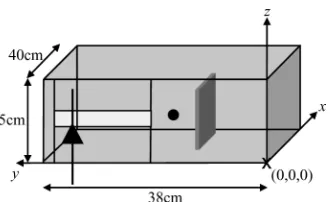
Fig. 1. FDTD simulation of shielded enclosure with an aperture containing a PCB.
system, the center of the dipole is at (−20, 26, 7), this is 20 cm away (in thex-direction) from the center of the aperture. The arms of the dipole are each 7 cm in length, with a radius of 1 mm. The voltage source at the center of the dipole has an amplitude ofV0 = 2V over a load of 50Ω. The input excitation is a Gaussian of the form
V =V0exp
−4 ln 2(t−t0)
2 f whh2
(42)
where t0 = 6.67×10⁻¹⁰ s is the onset time and f whh=
2.78×10⁻¹⁰s is the full width of the Gaussian pulse at half the height of the maximum amplitude.
The enclosure represents the shielding exterior of a typical electronic system containing a PCB. Using the coordinate sys-tem outlined before, the PCB is oriented in thex–zplane, ex-tending from the point (5, 14, 2) a distance xb = 30 cm in
the positive x-direction and a distance 10 cm in the positive z-direction. The components on the PCB will absorb some of the electric field that penetrates the enclosure and is incident upon the board. The PCB may, therefore, be modeled as a thin dielectric block with a reflection coefficient [18]. For this exam-ple, the reflection coefficientΓ is uniformly distributed in the interval
Γ = [−0.91,−0.97]. (43)
This reflection coefficient is optimized for a frequency of 1.8 GHz by changing the material parameters of the PCB. The reflection coefficient will, however, be accurate for a small fre-quency range around 1.8 GHz. Note that the reflection coeffi-cient described by (43) is uncertain, and it follows a uniform distribution. The uncertainty in this input will cause there to be an uncertainty in the output.
The output z-component of the electric field is observed at the center of the box. An FDTD simulation was used to obtain the normalized electric field at this point using a uniform cell size of 0.01 m.
Fig. 2 shows the mean output electric field with 95% confi-dence intervals (CIs), as predicted by the MCM. Figures, such as this one, are extremely useful when determining the quan-titative level of confidence that may be held in the results of a simulation. At 1.8 GHz, the 95% CI areEz = [0.418,0.444]
V/m. Thus, 95% of the sampled data was within about±3%of the mean value.
[image:8.594.313.551.66.196.2]The uncertainty in the output electric field is shown in Fig. 3. The uncertainties predicted by all three methods are in very
Fig. 2. Mean normalized electric field at the center of the shielded enclosure and the 95% CI.
Fig. 3. Uncertainty in the normalized electric field, at the center of the shielded enclosure, formed via the three UA methods.
good agreement. The uncertainty curves were compared using the FSV method over frequencies up to 3 GHz. The uncertainty predicted by the PCM is a “very good” match to the uncertainty predicted by the MCM, with a GDM of 2.3568. The MoM per-forms even better, and the frequency response of the uncertainty formed from the MoM and the MCM is an “excellent” match, having a GDM of 1.4755. Therefore, for this example, both ef-ficient UA methods provide uncertainty estimates that are very close to the uncertainty formed using the MCM.
IV. EXAMPLE2: A DIELECTRICSPHERE
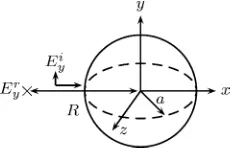
This example considers the reflection of a uniform plane wave off a dielectric sphere in free space. The incident electric field Ei
ypropagates in the positivex-direction, and is polarized in the y-direction with a magnitudeE0 = 1V/m. They-component of the backscattered fieldEr
y is calculated at a distance R=
0.2m from the center of the sphere. This backscattered electric field is normalized relative to the input excitation to form the normalized electric field. This backscattered field may be solved analytically using the Mie series [19].
In this example, the sphere parameters are uncertain: the ra-dius is normally distributed with a mean ¯a= 0.1 m and an uncertaintyσa= 0.005m, the relative permittivity is uniformly
distributed in the intervalǫr= [3.7,4.3], and the relative
perme-ability is uniformly distributed in the intervalµr = [0.95,1.05].
These uncertain input parameters will produce an uncertainty in
[image:8.594.311.551.240.373.2]EDWARDSet al.: UNCERTAINTY ANALYSES IN THE FDTD METHOD 161
[image:9.594.106.222.66.141.2]Fig. 4. Three-dimensional problem space containing a dielectric sphere. A uniform plane wave is reflected off the sphere and observed at X.
Fig. 5. Uncertainty in the normalized field backscattered from a dielectric sphere.
the output normalized electric field. The setup of this example is shown in Fig. 4.
The normalized electric field in the frequency domain was calculated using FDTD simulations, with a uniform broad Gaussian incident plane wave and a uniform cell size of 0.005 m. Fig. 5 shows the uncertainty in the FDTD simulations calculated using the three UA methods. At the lower frequencies, the uncer-tainties produced by the three methods are in good agreement. However, at the higher frequencies, both the PCM and the MoM overestimate the uncertainty, when compared to the uncertainty produced by the MCM. These qualitative comparisons are con-firmed using the FSV method. The PCM gives a “fair” estimate of the MCM uncertainty up to 1.02 GHz, and a “poor” estimate of the uncertainty between 1.02 and 3 GHz. The MoM does slightly better at the lower frequencies, providing a “fair” esti-mate of the MCM uncertainty up to 1.21 GHz. At the higher frequencies, however, the MoM performs less well, with a “very poor” estimate of the uncertainty between 1.21 and 3 GHz.
[image:9.594.45.282.183.315.2]Fig. 6 shows the normalized electric field produced from an FDTD simulation using the mean input parameter values and a simulation with the sphere radius perturbed by 5 mm. The two curves in this figure have similar resonant features, but are shifted slightly in the frequency domain. At 1 GHz, the fre-quency response curve is less resonant in nature. Changing the radius of the sphere causes a frequency shift, which, in turn, changes the value of the normalized electric field in a quasi-linear fashion, at this frequency. Changing the radius of the sphere at a more resonant frequency (e.g., 2.71 GHz) results in a frequency shift that causes a large nonlinear change in the normalized electric field. Fig. 7 shows the relationship be-tween the normalized electric field and the radius of the sphere at 1 and 2.71 GHz (calculated using the Mie series solution),
[image:9.594.310.544.257.389.2]Fig. 6. Normalized field backscattered from two dielectric spheres with dif-ferent radii.
Fig. 7. Normalized electric field backscattered from dielectric spheres with different radii at 1 and 2.71 GHz.
respectively. At 1 GHz, the normalized electric field depends on the radius in a relatively linear fashion, whereas at 2.71 GHz, the normalized electric field depends on the radius in a highly nonlinear manner. Similar nonlinear relationships between the output electric field and the other uncertain inputs arise at fre-quencies where there is a high modal density.
162 IEEE TRANSACTIONS ON ELECTROMAGNETIC COMPATIBILITY, VOL. 52, NO. 1, FEBRUARY 2010
TABLE I
COMPUTATIONALREQUIREMENTS OF THETHREEMETHODS
V. COMPUTATIONALREQUIREMENTS
Table I shows the computational performance of the three methods. All FDTD simulations were performed on a computer with a Pentium 4 processor running at 3.0 GHz. The table shows that the MoM requires the least amount of computational ex-pense. The MCM requires much more computational runtime than the PCM and the MoM, highlighting the need for efficient methods of quantifying the uncertainty in CEM simulations.
Table I displays the extra computational memory required by the PCM, compared to that required by the MCM and the MoM. In the second example, significantly, more memory is required for the PCM. The MCM and the MoM use an optimized FDTD method; the material parameter values are not stored at each point in the problem space, but a reference to the parameter value is stored. Conversely, for the PCM, material values need to be stored at all points in the problem space. The uncertainty in the sphere radius causes the material parameter inner product values, used by the PCM, to be different at different points in the problem space. This means that the full inner product values have to be stored at each point in the problem space, requiring significantly more memory. In more complex examples, the computational memory requirements may be too large to allow the PCM to be used.
To obtain the uncertainty of these (and any other) CEM sim-ulations, extra computational runtime is needed. This extra rtime will be significant for complex problems with many un-certain input parameters. Unun-certainty budgets provide essential information to help determine whether the results of a mea-surement are acceptable, and should not be discounted because of the extra computational expense. This paper has investigated two efficient UA methods (the PCM and the MoM), highlighting some of the strengths and limitations of these methods.
The efficient MoM and the PCM provided poor estimates of the output uncertainty when the relationship between the output and the uncertain inputs was nonlinear. It is generally accepted that the MCM provides a benchmark method of deter-mining output uncertainty with a good degree of accuracy. This method does not rely on any assumption on the relationship between the uncertain inputs and the output of the computa-tional simulations. The MCM, therefore, does not suffer from the nonlinear nature of EMC data. The MCM is, however, more computationally expensive than the MoM and the PCM. Since the uncertainty in the output of a computational scenario should be similar despite the CEM technique used, it may be possible to use a computationally efficient CEM technique (such as the
intermediate-level circuit model (ILCM) [20]), along with the MCM to provide an accurate estimate of the output uncertainty with relatively little computational expense. The ILCM method, for example, was able to find the shielding effectiveness of an enclosure over 3900 times faster than TLM simulations. To de-termine whether an accurate and efficient UA can be formed in this way, the uncertainty in the output of an EMC scenario must be shown to be relatively independent of the CEM technique used to model the scenario. This provides a promising avenue for future work in this area.
VI. CONCLUSION
Estimates of the uncertainty in the results of CEM simulations provide the scientific community with the quantitative level of confidence that may be held in the results. In the first example of this paper, it may be concluded that there is a 95% chance that the output value lies within 3% of its mean value. It is impossible to determine this level of confidence without performing an UA. This paper introduced three UA methods that were used to quantify the uncertainty in FDTD simulations. The novel im-plementation of the PCM required a modification of the FDTD algorithm. Of the three methods, the MoM was shown to be the computationally cheapest method. The PCM was shown to be computationally faster than the MCM, but required significantly more computational memory.
The MCM has been previously used to provide reliable esti-mates of uncertainty. The first example in this paper highlighted that the computationally cheaper MoM and PCM can give very good estimations of the uncertainty formed via the MCM. The efficient MoM and PCM, implemented in this paper, both rely on the assumption that the output of interest depends linearly on the uncertain inputs. In the second example, it was shown that this assumption is valid at subresonant frequencies, but poorer at fre-quencies with a higher density of resonant modes. This reflected the uncertainty estimates formed by the PCM and the MoM, for this example, which were better at subresonant frequencies. In conclusion, the MoM and the PCM may only provide moderate estimates of the uncertainty in resonant EMC data. However, the efficient methods have also been shown to work well at sub-resonant frequencies, for an example, with multiple uncertain inputs.
The MCM is generally accepted as being an accurate method for quantifying output uncertainties. The method does not rely on an assumed relationship between the uncertain inputs and the output of computational simulations, and therefore does not suffer from the resonant nature of EMC data. The MCM is also, however, known to be computationally expensive. It has been suggested that a fruitful avenue for future work may be to use the MCM with a computationally efficient CEM technique (such as the ILCM [20]) to provide an accurate estimate of the output uncertainty with relatively little computational expense.
ACKNOWLEDGMENT
The PCM bears no relation to chaos theory, and the MoM used in this paper should not be confused with the common method
EDWARDSet al.: UNCERTAINTY ANALYSES IN THE FDTD METHOD 163
used in CEM. Both of these methods are statistical methods that may be used to quantify uncertainty.
REFERENCES
[1] C. Chauvi`ere, J. S. Hesthaven, and L. Lurati, “Computational modeling of uncertainty in time-domain electromagnetics,” SIAM J. Sci. Comput., vol. 28, no. 2, pp. 751–775, Jul. 2006.
[2] A. Ajayi, P. Ingrey, P. Sewell, and C. Christopolous, “Direct computa-tion of statistical variacomputa-tions in electromagnetic problems,” IEEE Trans. Electromagn. Compat., vol. 50, no. 2, pp. 751–775, May 2008. [3] J. Pereira, L. de Menezes, and A. Borges, “Statistical analysis of induced
ground voltage using the TLM+UT method,” inProc. IEEE Int. Symp. Electromagn. Compat. (EMC 2008), pp. 1–4.
[4] L. de Menezes, A. Ajayi, C. Christopoulos, P. Sewell, and G. A. Borges, “Efficient extraction of statistical moments in electromagnetic problems solved with the method of moments,” inProc. SBMO/IEEE MTT-S Int. Microw. Optoelectron. Conf. (IMOC 2007), pp. 757–760.
[5] ISO,Guide to the Expression of Uncertainty in Measurement, Int. Stan-dards Org., Geneva, Switzerland, 1993.
[6] UKAS,The Expression of Uncertainty in EMC Testing,1st ed. Middlesex, U.K.: UKAS Publication LAB 34, 2002.
[7] A. P. Duffy, A. J. M. Martin, A. Orlandi, G. Antonini, T. M. Benson, and M. S. Woolfson, “Feature selective vaidation (FSV) for validation of computational electromagnetics (CEM)—Part I: The FSV method,”IEEE Trans. Electromagn. Compat., vol. 48, no. 3, pp. 449–459, Aug. 2006. [8] A. P. Duffy, A. Orlandi, and H. Sasse, “Offset difference measure
en-hancement for the feature-selective validation method,” IEEE Trans. Electromagn. Compat., vol. 50, no. 2, pp. 413–415, May 2008. [9] Draft Standard for Validation of Computational Electromagnetics
Com-puter Modeling and Simulations, IEEE Standards P1597.1/D4.3, Jun. 2008.
[10] M. D. McKay, W. J. Conover, and R. J. Beckman, “A comparison of three methods for selecting values of input variables in the analysis of output from a computer code,” Technometrics, vol. 21, no. 2, pp. 239–245, May 1979.
[11] N. Wiener, “The homogeneous chaos,” Amer. J. Math., vol. 60, pp. 897– 936, 1938.
[12] D. B. Xiu and G. E. Karniadakis, “The Wiener-Askey polynomial chaos for stochastic differential equations,”SIAM J. Sci. Comput., vol. 24, no. 2, pp. 619–644, 2002.
[13] J. Faragher, “Probabilistic methods for the quantification of uncertainty and error in computational fluid dynamics simulations,” DSTO Air Ve-hicles Division, Melbourne, Vic., Australia, Tech. Rep. DSTO-TR-1633, 2004.
[14] D. B. Xiu and G. E. Karniadakis, “Modeling uncertainty in flow simu-lations via generalized polynomial chaos,” J. Comput. Phys., vol. 187, no. 1, pp. 137–167, 2003.
[15] O. M. Knio and O. P. Le Maˆıtre, “Uncertainty propagation in CFD us-ing polynomial chaos decomposition,” Fluid Dyn. Res., vol. 38, no. 9, pp. 616–640, 2006.
[16] K. S. Yee, “Numerical solution of initial boundary value problem involving Maxwell’s equations in isotropic media,”IEEE Trans. Antennas Propag., vol. AP14, no. 3, pp. 302–307, May 1966.
[17] G. Mur, “Absorbing boundary conditions for the finite-difference approxi-mation of the time-domain electromagnetic-field equations,”IEEE Trans. Electromagn. Compat., vol. EMC23, no. 4, pp. 377–382, Nov. 1981. [18] M. P. Robinson, S. J. Porter, and P. Op Gen Oorth, “Reflection and
trans-mission coefficients of printed circuit boards,” inProc. 4th Eur. Symp. Electromagn. Compat., Bruges, Sep. 11–15, 2000, pp. 209–213.
[19] G. Mie, “Beitr¨age zur Optik tr¨uber Medien, speziell kolloidaler Met-all¨osungen,” Ann. Der Phys., vol. 330, no. 3, pp. 377–445, 1908. [20] T. Konefal, J. F. Dawson, A. C. Marvin, M. P. Robinson, and S. J. Porter,
“A fast multiple mode intermediate level circuit model for the prediction of shielding effectiveness of a rectangular box containing a rectangular aperture,”IEEE Trans. Electromagn. Compat., vol. 47, no. 4, pp. 678–691, Nov. 2005.
Robert S. Edwardsreceived the M.Math. degree (with first-class honors) in mathematics and physics in 2005 and the Ph.D. degree in electronic engineer-ing, both from the University of York, York, U.K.
He is currently with the Department of Electron-ics, University of York. His research interests in-clude computational electromagnetics and statistical methods.
Dr. Edwards was the recipient of the P.B. Kennedy Prize and the Oliver Heavens Award in 2005 for achieving the highest academic record by an under-graduate in the Mathematics Department and the Physics Department, Univer-sity of York.
Andrew C. Marvin (M’83–SM’06) received the B.Eng., M.Eng., and Ph.D. degrees in electrical en-gineering from the University of Sheffield, Sheffield, U.K., between 1972 and 1978.
He is currently a Professor of Applied Electro-magnetics, a Leader of the Physical Layer Research Group, and the Deputy Head of the Department of Electronics, University of York, York, U.K., where he is also the Technical Director of York Electromag-netic Compatibility (EMC) Services Ltd. His current research interests include EMC measurement tech-niques and shielding.
Prof. Marvin is a Member of the Institution of Engineering and Technology. He represents U.K. on the International Union of Radio Science Commission A (Electromagnetic Metrology). He is a Co-Convenor of the International Special Committee on Radio Interference, the International Electrotechnical Commis-sion (IEC) Joint Task Force on the use of TEM cells for EMC measurements, the Vice-Chairman of the IEEE Std-299 Working Group on Shielding Effec-tiveness Measurement, and an Associate Editor of the IEEE TRANSACTIONS ON
ELECTROMAGNETICCOMPATIBILITY.
Stuart J. Porter (M’93) received the B.Sc. and D.Phil. degrees from the University of York, York, U.K., in 1985 and 1991, respectively.