This is a repository copy of A robust correlation analysis framework for imbalanced and dichotomous data with uncertainty.
White Rose Research Online URL for this paper: http://eprints.whiterose.ac.uk/134706/
Version: Accepted Version
Article:
Lai, CS orcid.org/0000-0002-4169-4438, Tao, Y, Xu, F et al. (7 more authors) (2019) A robust correlation analysis framework for imbalanced and dichotomous data with uncertainty. Information Sciences, 470. pp. 58-77. ISSN 0020-0255
https://doi.org/10.1016/j.ins.2018.08.017
© 2018 Elsevier Inc. This manuscript version is made available under the CC-BY-NC-ND 4.0 license http://creativecommons.org/licenses/by-nc-nd/4.0/.
[email protected] https://eprints.whiterose.ac.uk/ Reuse
This article is distributed under the terms of the Creative Commons Attribution-NonCommercial-NoDerivs (CC BY-NC-ND) licence. This licence only allows you to download this work and share it with others as long as you credit the authors, but you can’t change the article in any way or use it commercially. More
information and the full terms of the licence here: https://creativecommons.org/licenses/
Takedown
If you consider content in White Rose Research Online to be in breach of UK law, please notify us by
* Corresponding authors.
E-mail addresses: [email protected] (C.S. Lai), [email protected] (Y. Tao), [email protected] (F. Xu), [email protected] (W.W.Y. Ng), [email protected] (Y. Jia), [email protected] (H. Yuan), [email protected] (C. Huang), [email protected] (L.L. Lai), [email protected] (Z. Xu), [email protected] (G. Locatelli)
A robust correlation analysis framework for imbalanced and
1
dichotomous data with uncertainty
2 3
Chun Sing Lai a,b, Yingshan Tao a, Fangyuan Xu a,*, Wing W. Y. Ng c,*, Youwei Jia a,d,
4
Haoliang Yuan a, Chao Huang a, Loi Lei Lai a,*, Zhao Xu d, Giorgio Locatelli b
5
a Department of Electrical Engineering, School of Automation, Guangdong University of Technology, Guangzhou
6
510006, China 7
b School of Civil Engineering, Faculty of Engineering, University of Leeds, Woodhouse Lane, Leeds LS2 9JT,
8
U.K. 9
c Guangdong Provincial Key Lab of Computational Intelligence and Cyberspace Information, School of Computer
10
Science and Engineering, South China University of Technology, Guangzhou 510630, China 11
d Department of Electrical Engineering, The Hong Kong Polytechnic University, Hong Kong SAR, China
12 13 14
Abstract— Correlation analysis is one of the fundamental mathematical tools for identifying
15
dependence between classes. However, the accuracy of the analysis could be jeopardized due
16
to variance error in the data set. This paper provides a mathematical analysis of the impact of
17
imbalanced data concerning Pearson Product Moment Correlation (PPMC) analysis. To
18
alleviate this issue, the novel framework Robust Correlation Analysis Framework (RCAF) is
19
proposed to improve the correlation analysis accuracy. A review of the issues due to
20
imbalanced data and data uncertainty in machine learning is given. The proposed framework
21
is tested with in-depth analysis of real-life solar irradiance and weather condition data from
22
Johannesburg, South Africa. Additionally, comparisons of correlation analysis with prominent
23
sampling techniques, i.e., Synthetic Minority Over-Sampling Technique (SMOTE) and
24
Adaptive Synthetic (ADASYN) sampling techniques are conducted. Finally, K-Means and
25
Wards Agglomerative hierarchical clustering are performed to study the correlation results.
26
Compared to the traditional PPMC, RCAF can reduce the standard deviation of the correlation
27
coefficient under imbalanced data in the range of 32.5% to 93.02%.
28 29
Keywords— Pearson product-moment correlation, imbalanced data, clearness index,
30
dichotomous variable.
31 32
1. Introduction
33 34
With the exponential increase of the amount of data introduced by an increasing number of
35
physical devices, the large-scale advent of incomplete and uncertain data is inevitable, such as
36
those from smart grids (Lai and Lai, 2015; Wu et al., 2014). For sparse data, the number of
37
data points is inadequate for making a reliable judgement. This has been an issue for the
38
successful delivery of megaprojects (Locatelli et al., 2017). In machine learning and data
39
mining applications, redundant data can seriously deteriorate the reliability of models trained
40
from the data.
41
Data uncertainty is a phenomenon in which each data point is not deterministic but subject
42
to some error distributions and randomness. This is introduced by noise and can be attributed
43
to inaccurate data readings and collections. For example, data produced from GPS equipment
44
are of uncertain nature. The data precision is constrained by the technology limitations of the
45
GPS device. Hence, there is a need to include the mean value and variance in the sampling
46
location to indicate the expected error. A survey of state-of-the-art solutions to imbalanced
47
learning problems is provided in (He and Garcia, 2009). The major opportunities and
48
challenges for learning from imbalanced data are also highlighted in (He and Garcia, 2009).
The number of publications on imbalanced learning has increased by 20 times from 1997 to
50
2007. Imbalanced data can be classified into two categories, namely, intrinsic and extrinsic
51
imbalanced. Intrinsic imbalance is due to the nature of the data space, whereas extrinsic
52
imbalance is not. Given a dataset sampled from a continuous data stream of balanced data with
53
respect to a specific period of time; if the transmission has irregular disturbances that do not
54
allow the data to be transmitted during this period of time, the missing data in the dataset will
55
result in an extrinsic imbalanced situation obtained from a balanced data space. An example of
56
intrinsic imbalanced could be due to the difference in the number of samples of different
57
weather conditions, i.e., in general, the ‘Clear’ weather condition has the most occurrences
58
throughout the year, whereas ‘Snow’ may only have a few occurrences.
59
There is a growth of interest in class imbalanced problems recently due to the classification
60
difficulty caused by the imbalanced class distributions (Wang and Yao, 2012; Xiao et al.,
61
2017). To solve this problem, several ensemble methods have been proposed to handle such
62
imbalances. Class imbalances degrade the performance of the derived classifier and the
63
effectiveness of selections to enhance classifier performance (Malof et al., 2012).
64
This paper proposes and validates a new framework for the impact of imbalanced data on
65
correlation analysis. The impact of imbalanced data is described using a mathematical
66
formulation. Additionally, RCAF is proposed for correlation analysis with the aim of reducing
67
the negative effects due to an imbalanced ratio. This will be investigated with a theoretical and
68
real-life case study.
69
Section 2 provides a literature review on the imbalanced data problem, followed by the
70
correlation analysis of imbalanced data. Section 3 provides an overview of the critical features
71
and the impacts on correlation analysis. Simulations will be conducted to support the findings.
72
Section 4 proposes a new framework for the correlation analysis. Section 5 provides a real-life
73
case study, based on solar irradiance and weather conditions, to evaluate the new framework.
74
Different imbalanced data sampling techniques will be used to compare the correlation analysis
75
performance. Cluster analysis of weather conditions will be given to understand the
76
implications of the correlation results. Future work and conclusions will be given in Section 6.
77 78
2. Correlation analysis and imbalanced data
79 80
2.1. Imbalanced classification problems
81 82
Imbalanced data refers to unequal variable sampling values in a dataset. For example, 90%
83
of sampling data can be in the majority class, with only 10% of the sampling data in the
84
minority class. Therefore, the imbalanced ratio is 9:1. Imbalanced data appears in many
85
research areas. As mentioned in (Krstic and Bjelica, 2015), when TV recommender systems
86
perform well, the number of interactions for users to express positive feedback is anticipated
87
to be greater than the number of negative interactions on the recommended content. This is
88
known as class imbalanced. The misclassification of the unwanted content can be recognized
89
by TV viewers easily, therefore, system performance could decrease.
90
Commonly, modifying imbalanced datasets to provide a balanced distribution is carried out
91
using sampling methods (Li et al., 2010; Liu et al., 2009; Wang and Yao, 2012). From a broader
92
perspective, over-sampling and under-sampling techniques seem to be functionally equivalent,
93
since they both can provide the same proportion of balance by changing the size of the original
94
dataset. In practice, each technique introduces challenges that can affect learning. The major
95
issue with under-sampling is straightforward, classifiers will miss important information in
96
respect to the majority class, by removing examples from the majority class (Ng et al., 2015).
97
The issues regarding over-sampling are less straightforward. Since over-sampling adds
98
replicated data to the original dataset, multiple instances of certain samples become ‘tied’,
resulting in overfitting. As proposed in (Mease et al., 2007), one solution to the over-sampling
100
problem is to add a small amount of random noise to the predictor so the replicates are not
101
duplicated, which can minimize overfitting. This jittering adds undesirable noise to the dataset
102
but the negative impact of imbalanced datasets has been shown to be reduced. Under-sampling
103
is a favoured technique for class-imbalanced problems; it is very efficient since only a subset
104
of the majority class is used. The main problem with this technique is that many majority class
105
examples are ignored.
106
Class imbalanced learning is employed to resolve supervised learning problems in which
107
some classes have significantly more samples than others (Xiao et al., 2017). The study of
108
multiclass imbalanced problems and the Dynamic Sampling method (DyS) for multilayer
109
perceptron are provided in (Lin et al., 2013). The authors claim that the DyS method could
110
outperform the pre-sample methods and active learning methods for most datasets. However,
111
a theoretical foundation is necessary to explain the reason a simple method such as DyS could
112
perform so well in practice.
113
Support Vector Machine (SVM) is a popular machine learning technique that works
114
effectively with balanced datasets (Batuwita and Palade, 2010; Tang et al., 2009). However,
115
with imbalanced datasets, suboptimal classification models are produced with SVMs.
116
Currently, most research efforts in imbalanced learning focus on specific algorithms and/or
117
case studies. Many researchers use machine learning methods such as support vector machines
118
(Batuwita and Palade, 2010), cluster analysis (Diamantini and Potena, 2009), decision tree
119
learning (Mease et al., 2007; Weiss and Provost, 2003), neural networks (Yeung et al., 2016;
120
Zhang and Hu, 2014; Zhou and Liu, 2006), etc., with a mixture of over-sampling and
under-121
sampling techniques to overcome the imbalanced data problems (Liu et al., 2009; Seiffert et
122
al., 2010). A novel machine learning approach to assess the quality of sensor data using an
123
ensemble classification framework is presented in (Rahman et al., 2014), in which a
cluster-124
oriented sampling approach is used to overcome the imbalance issue.
125
The issues of class imbalanced learning methods and how they can benefit software defect
126
prediction are given in (Wang and Yao, 2013). Different categories of class imbalanced
127
learning techniques, including resampling, threshold moving and ensemble algorithms, have
128
been studied for this purpose. Medical data are typically composed of ‘normal’ samples with
129
only a small proportion of ‘abnormal’ cases, which leads to class imbalanced problems (Li et
130
al., 2010). Constructing a learning model with all the data in class imbalanced problems will
131
normally result in a learning bias towards the majority class.
132
Imbalanced data can influence the feature selection results. As mentioned in (Zhang et al.,
133
2016), traditional feature selection techniques assume the testing and training datasets follow
134
the same data distribution. This may decrease the performance of the classifier for the
135
application of adversarial attacks in cybersecurity. For real-life applications, the distribution of
136
different datasets and variables may be significantly different and should be thoroughly studied.
137
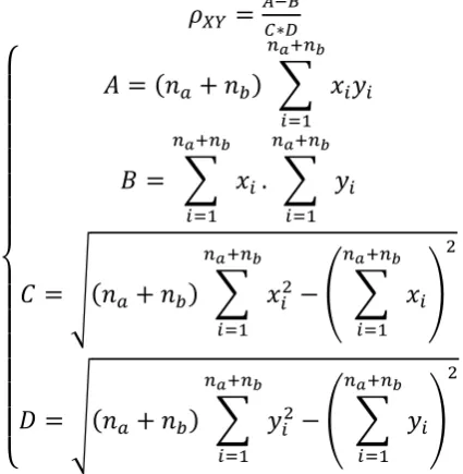
Feature selection based on methods such as feature similarity measure (Mitra et al., 2002),
138
harmony search (Diao et al., 2014; Diao and Shen, 2012), hybrid genetic algorithms (Oh et al.,
139
2004), dependency margin (Liu et al., 2015b), cluster analysis (Chow et al., 2008) has been
140
developed. The methods have contributed to the quality enhancement of feature selection.
141
However, the fundamental issues of the uncertainty and imbalanced ratio in datasets have not
142
been studied.
143 144
2.2. Correlation analysis for imbalanced data problems
145 146
Many correlation analyses have been conducted on imbalanced datasets. For example,
147
Community Question Answering (CQA) is a platform for information seeking and sharing. In
148
CQA websites, participants can ask and answer questions. Feedback can be provided in the
manner of voting or commenting. (Yao et al., 2015) proposed an early detection method for
150
high-quality CQA questions/answers. Questions of significant importance that would be
151
widely recognized by the participants can be identified. Additionally, helpful answers that
152
would attain a large amount of positive feedback from participants can be discovered. The
153
correlation of questions and answers was performed with Pearson R correlation to test the
154
dependency of the voting score. The classification accuracy with imbalanced data, i.e., the ratio
155
between the number of data for positive and negative feedbacks have not been addressed.
156
Gamma coefficient is a well-known rank correlation measure that is frequently used to
157
quantify the strength of dependency between two variables in ordinal scale (Ruiz and
158
Hüllermeier, 2012). To increase the robustness of this measure in data with noise, Ruiz et al.
159
(Ruiz and Hüllermeier, 2012) studied the generalization of the gamma coefficient based on
160
fuzzy order relations. The fuzzy gamma has been shown to be advantageous in the presence of
161
noisy data. However, the authors did not consider the imbalanced data issue for correlation
162
analysis.
163
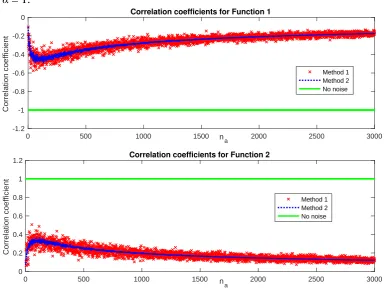
In clinical studies, the linear correlation coefficient is frequently used to quantify the
164
dependency between two variables, e.g., weight and height. The correlation can indicate if a
165
strong dependency exists. However, in practice, clinical data consists of a latent variable with
166
the addition of an inevitable measurement error component, which affects the reproducibility
167
of the test. The correlation will be less than one even if the underlying physical variables are
168
perfectly correlated. Francis et al. (Francis et al., 1999) studied the reduction in correlation due
169
to limited reproducibility. The implications of experimental design and interpretation were also
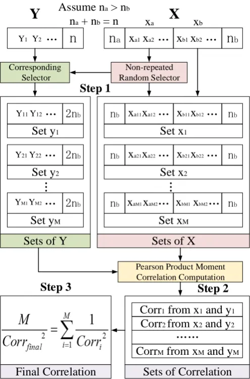
170
discussed. It is confirmed that with large measurement errors, the measured correlation for
171
perfectly correlated variables cannot be equal to one but must be less than one (Francis et al.,
172
1999). Francis et al. (Francis et al., 1999) described a method which allows this effect to be
173
quantified once the reproducibility of the individual measurements is known. However, the
174
paper has not resolved the correlation inaccuracy problem and only provides an indication of
175
the effect of noise on the correlation in an imbalanced dataset. The paper concludes that the
176
designers of experiments can relieve the problem of attenuation of correlation in two ways.
177
First, the random component of the error should be minimized, with the aim of improving
178
reproducibility. Technical advances may allow this to occur, but relying on them is not always
179
practical. Random measurement error can also be attenuated statistically but this requires care
180
and logical judgement. Note that some variance errors in the data are inevitable, such as solar
181
irradiance where unexpected phenomenon such as birds flying cannot be avoided.
182 183
3. Impact of imbalanced ratio and uncertainty on correlation analysis
184 185
Classes exist in various machine learning models and can be in the form of dichotomous
186
variables. The features can be represented by binary classification, i.e., 0 or 1. For example,
187
different weather conditions for solar irradiance prediction can be classified (0 for ‘Clear’ and
188
1 for ‘Rain’).
189 190
3.1. Correlation analysis for imbalanced dichotomous data with uncertainty introduced by
191
noise
192 193
In statistical analysis, dependency is defined as the degree of statistical relationship between
194
two sets of data or variables. Dependency can be calculated and represented by correlation
195
analysis. The most commonly used formula is parametric and known as the Pearson Product
196
Moment Correlation (PPMC) coefficient. By definition, the PPMC coefficient has a range from
197
the perfect negative correlation of negative 1.0 to the perfect positive correlation of positive
198
1.0, with 0 representing no correlation (Mitra et al., 2002).
The following problem is used to describe this research issue.
200
Assumption: Given two variables X and Y, where . In the obtained
201
sampling dataset, the number of samples in is and the number of samples in is ,
202
with The noise, i.e., sampling error, occurs in Y. The relationship between each
203
value of Y ( ) and each value of X is , . Each noise
204
follows a certain distribution K with mean error . The square of noise error Erri2 follows
205
the distribution L with mean square error .
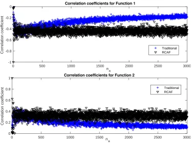
206
Fig. 1 presents the PPMC correlation with a variable, i.e., weather being dichotomous. The
207
regression line depicts a negative correlation between Clearness Index (CI) and the two weather
208
conditions. This means the weather transition from ‘Clear’ to ‘Mostly Cloudy’ will reduce the
209
amount of solar resources received.
210 211
[image:6.595.192.405.550.768.2]212
Fig. 1. Correlation analysis with a dichotomous variable.
213 214
The PPMC coefficient is given in Equation (1) below:
215 216
217
218
For C to become zero, possible factors include and all are zero. Based on Fig.
220
1, if there is no data, i.e., and the sample size is zero, it is impossible to conduct the
221
correlation. All equal to zero signifies there is no value in the variable. Similarly, for D to
222
become zero, possible factors include and all y are zero. The average value of
223
the sampling set is equal to the expectation of the distribution. Equation (2) depicts this
224
relationship while Equations (3) and (4) are true.
225 226
227
228
229
230
By considering yi = f(xi) + Erri in Equation (1), further expressions are presented in Equation
231
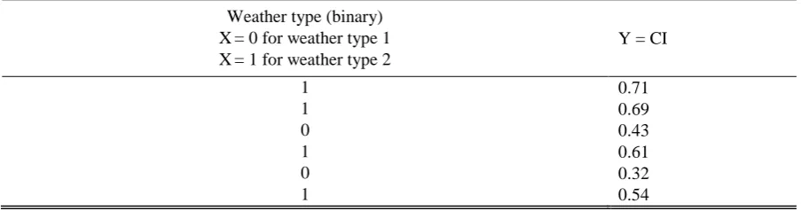
(5).
232
233
234
By considering = * , where is the number ratio between value and value ,
235
Equation (5) can be transformed into Equation (6).
236
237
238
If ≠ and f( ) ≠ f( ), the type of correlation can be expressed by Equation (7).
239 240
241
242
Equation (6) shows the correlation may not be +1/-1 given there is an increasing/decreasing
243
linear relationship between X and Y. It is also related to the Momentum Ratio R. For the case
244
, based on Fig. 1, this means the “actual” (excluding error variance) CI for
245
‘Clear’ is the same as the actual CI for ‘Mostly Cloudy’. Since the variance of Y is zero, the
246
denominator is zero which makes the correlation coefficient undefined.
247 248 249
3.2. Impact of imbalanced ratio
250 251
The imbalanced ratio in the dataset is presented by in Equation (7). Equation (8) extracts
252
the section of R in Equation (7) as given below:
254
In Equation (8), the minimum point occurs at = 1. This indicates R is maximized if the
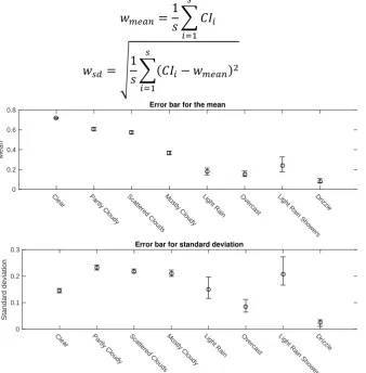
255
sampling dataset contains an equal number of and . In this section, two functions are
256
employed to study the imbalanced datasets and the correctness of Equation (7). Equation (9)
257
introduces the two functions. The error of each sampling point is assumed to follow a standard
258
normal distribution The first function in Equation (9) establishes a negative
259
relationship while the second function establishes a positive relationship. The correlation can
260
be computed using two methods. Method 1 uses the derived Equation (7) and Method 2 uses
261
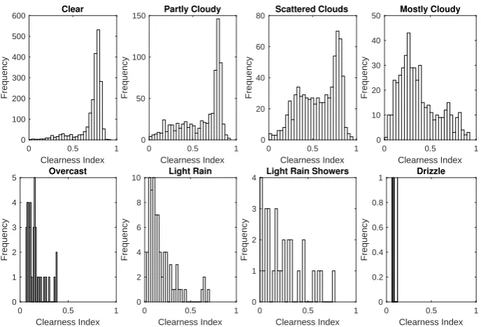
the conventional Equation (1).
262 263
sin
ln (9) 264
[image:8.595.106.491.364.652.2]265
Fig. 2 shows the simulation results for the two functions in Equation (9). is fixed at 100
266
and a sensitivity analysis is conducted for from 1 to 3000. For Function 2, the correlation
267
absolute value increases from 1 to 100 and decreases from 100 to 3000. This shows that
268
Method 1 and Method 2 produce similar results. The simulations in Fig. 2 have proved that
269
Equation (7) is valid. The maximum absolute value of the correlation occurs at = = 100,
270
where = 1.
271
272
Fig. 2. Correlation for the two functions with imbalanced dataset.
273 274
Fig. 2 indicates that although variables X and Y have a confirmed dependence, the correlation
275
may be distorted by imbalanced data. The reason the correlations obtained from Method 1 have
276
more fluctuations than Method 2 is due to the assumption made with Equation (2). A general
277
recognition of correlation with high dependency is usually between 0.7 and 1.0, neutral
278
dependency is between 0.3 and 0.7, and low dependency is between 0 and 0.3. However, for
279
Function 2 in Equation (9), the correlation reaches 0.12 when na is 3000 ( = 30), which is far
280
0 500 1000 1500 na 2000 2500 3000
-1.2 -1 -0.8 -0.6 -0.4 -0.2 0
C
o
rr
e
la
ti
o
n
c
o
e
ff
ic
ie
n
t
Correlation coefficients for Function 1
Method 1 Method 2 No noise
0 500 1000 1500 n 2000 2500 3000
a 0
0.2 0.4 0.6 0.8 1 1.2
C
o
rr
e
la
ti
o
n
c
o
e
ff
ic
ie
n
t
Correlation coefficients for Function 2
from the maximum value 0.37. This may misinterpret the correlation from ‘neutral dependency’
281
to ‘low dependency’. The optimal correlation can be realized when the datasets have equal
282
sizes.
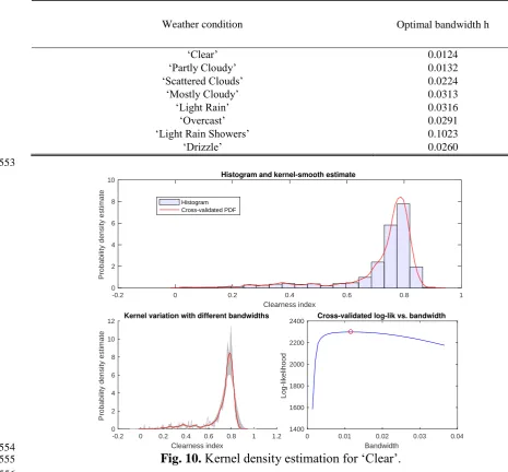
283 284
3.3. Impact of noise
285 286
The contribution of noise to the correlation is presented by Equation (10). Noise represents
287
an unconsidered impact that can cause deviation from the actual value of a variable, which
288
contributes to variance error. It can be recognized as the inaccuracy of measured data.
289 290
291
As shown in Equation (7), correlation may be distorted by the imbalanced ratio, with an
292
exceptional condition that in Equation (10) is equal to zero. If all noise is rejected by
293
a perfect sensor, Equation (7) indicates the correlation will not be influenced by an imbalanced
294
ratio and the resultant Momentum Ratio becomes 1. A simulation is conducted with Equation
295
(9) without noise. The correlation results without noise are presented in Fig. 2. The
296
correlations of the two functions in Equation (9) are shown to be perfectly correlated, i.e., 1
297
(or -1) when noise does not exist. As increases, the no-noise correlations maintain a value
298
of 1 (or -1). This phenomenon indicates the imbalanced ratio does not influence correlation
299
when noise is removed. Noise is one of the key factors that affect correlation with respect to
300
the imbalanced ratio.
301 302
3.4. Impact of output differences
303 304
The contribution of the output difference to correlation is presented by Equation (11).
305
306
In Equation (9), decreases and R in Equation (7) increases if the difference
307
between and increases. This indicates that R can be controlled by the output
308
difference. A larger output difference can counteract the effect of an imbalanced ratio. Similar
309
to Equation (7), for the case , the correlation coefficient is undefined when the
310
variance of Y is zero.
311
sin
ln 312
Fig. 3 presents the simulation results for Equation (12). Note that
313
increases as increases. In addition, the correlation at the same imbalanced ratio is closer to
314
a strong correlation (1 or -1) with an increased . This indicates that a larger output difference
315
may increase R and counteract the impact of imbalance.
318
Fig. 3. Correlation on specified function with imbalanced dataset.
319 320
4. Robust correlation analysis framework
321 322
4.1. Framework
323
This paper introduces a novel correlation analysis framework to alleviate the negative impact
324
of imbalanced data with noise in correlation analysis. Fig. 4 presents the structure of the
325
framework. In Fig. 4, X has two values ( , ) in the sampling dataset. The number of data
326
points in and are and ,respectively. Each x value and its corresponding y value
327
construct a data pair (x, y). The correlation analysis framework consists of the following two
328
main steps:
329
Step 1: Creating groups of balanced datasets: The first step is to determine which
330
variable X has the largest amount of data. For example, is selected if , then,
331
select amount of and combine them into pairs with . In this dataset, the number of
332
data points in and is equal to . The procedure is repeated M times to construct a
333
group of balanced sets. To prevent the loss of information from the removal of data and to
334
fully utilize all the data, the method to determine M is shown in Equation (13). In the
non-335
repeated random selector, sampling without replacement is used for sampling purposes to
336
prevent ‘tied’ data. The ceil function is used to round the value M towards positive infinity.
337
338
Step 2: Correlation integration: Corri, which is non-zero, is the correlation of a balance
339
set calculated with Equation (1). Assume there are M balanced sets, the final correlation
340
can be computed by Equation (14) as below:
341
342
343
Table 1 presents the detailed algorithm for RCAF. The implementation and pseudocode were
344
developed with MATLAB.
345 346
0 200 400 n 600 800 1000
a
-1.2 -1 -0.8 -0.6 -0.4 -0.2 0
C
o
rr
e
la
ti
o
n
c
o
e
ff
ic
ie
n
t
Correlation coefficients for Function 1
Beta = 1 Beta = 3 Beta = 5 Beta = 9
0 200 400 600 800 1000
na 0
0.2 0.4 0.6 0.8 1 1.2
C
o
rr
e
la
ti
o
n
c
o
e
ff
ic
ie
n
t
Table 1
347
Algorithm for RCAF.
348
As depicted in Table 1, the computational complexity (CC) for RCAF is relatively low.
349
According to Equation (1), the CC for PPMC is linear (Liu et al., 2016) at with data size
350
. Since RCAF consists of converting the majority class datainto M datasets, with each dataset
351
having the size of the minority class, the CC for RCAF is approximately or .
352
Although RCAF has a higher CC due to additional computations, e.g., Equations (13) and (14)
353
and the requirement of more data storage, the improved correlation analysis under imbalanced
354
data can justify the use of RCAF.
355 356 357 358
Input:
size size zeros zeros
Output:
corr final PPMC for and
Algorithm:
If is negative % Use Eq. (1) to determine if the correlation is positive or negative.
sign = -1;
else
sign = +1;
end
If then
ceil
For counter
posi randperm posi posi
cori counter corr Eq
cori counter cori counter
end else
ceil
For counter
posi randperm posi posi
cori counter corr Eq
cori counter cori counter
end end
reg mean cori
359
Fig. 4. Robust correlation analysis framework.
360 361
4.2. Proof of RCAF effectiveness
362 363
The Momentum Ratio R should be maximized as explained above. In Step 2 of RCAF, R is
364
calculated with correlations from all balanced sets, as shown in Equation (15). mse_i denotes
365
the mse of each balanced set. me_i denotes the me of each balanced set. i is of each balanced
366
set.
367
368
For each balanced dataset, since the number of data points in and are equal, = 1.
369
Equation (15) can be rewritten as Equation (16).
370 371
372
Assuming the sample size, i.e., is large, the noise terms in Equation (16) can be expressed
373
as Equation (17).
374 375
Assume na > nb
na + nb = n
X
n
an
bNon-repeated Random Selector
nb
Set x1
nb
n
Corresponding Selector
2nb
Sets of X
2nb
2nb
Set y1
Set y2
Set yM
Sets of Y
Sets of Correlation Corr1 from x1 and y1
Corr2 from x2 and y2
CorrM from xM and yM
Final Correlation
Y
Pearson Product Moment
Correlation Computation
nb
Set x2
nb
nb
Set xM
nb
Step 1
Step 2 Step 3
xa xb
xb1xb2 Y1 Y2
Y11Y12
Y21Y22
YM1YM2
xa1xa2
xa11xa12
xa21xa22
xaM1xaM2
xb11xb12
xb21xb22
376
377
By considering Equations (7), (16), and (17); Equation (18) gives the equations of R for the
378
original correlation and the new correlation. Note that the term disappears in the Momentum
379
Ratio under RCAF.
380
381
382
383 384 385
4.3. Theoretical study stimulations
386 387
Base on Equation (9), the correlations under RCAF are much more stable and slanting does
388
not occur with respect to the increase of the imbalanced ratio. Fig. 5 shows the simulation
389
results. The imbalanced ratio increases as increases. However, the correlations under RCAF
390
do not have a large variation and the optimal value is maintained.
391 392
[image:13.595.112.489.462.742.2]393
Fig. 5. Correlation comparison between traditional approach and RCAF.
394
0 500 1000 1500 2000 2500 3000
na
-1 -0.8 -0.6 -0.4 -0.2 0
C
o
rr
e
la
ti
o
n
c
o
e
ff
ic
ie
n
t
Correlation coefficients for Function 1
Traditional RCAF
0 500 1000 1500 n 2000 2500 3000
a 0
0.2 0.4 0.6 0.8 1
C
o
rr
e
la
ti
o
n
c
o
e
ff
ic
ie
n
t
Correlation coefficients for Function 2
5. Real-life case study: correlation for weather conditions and clearness index
395 396
5.1. Problem context and correlation analysis
397 398
Weather condition is one of the major factors affecting the amount of solar irradiance
399
reaching earth. As a consequence, one of the most important applications affected by solar
400
irradiance due to weather perturbation is Photovoltaic (PV) system. Weather condition changes
401
affect the electrical power generated by a PV system with respect to time.
402
Using CI in Equation (19) is one method to evaluate the influence of weather conditions with
403
respect to solar irradiance (Lai et al., 2017a). The analysis of these fluctuations with regard to
404
solar energy applications should focus on the instantaneous CI (Kheradmanda et al., 2016; Liu
405
et al., 2015a; Woyte et al., 2007; Woyte et al., 2006). CI can effectively characterize the
406
attenuating impact of the atmosphere on solar irradiance by specifying the proportion of
extra-407
terrestrial solar radiation that reaches the surface of the earth. In Equation (19) for each time of
408
the year, is the irradiance on the surface of the earth measured with a pyranometer
409
device and is the clear-sky solar irradiance (Lai et al., 2017a). The CI value will be
410
between 0 and 1, where 0 and 1 indicate no solar irradiance and the maximum amount of solar
411
irradiance will arrive on the surface of earth, respectively. This index can be used to quantify
412
the amount of atmospheric fluctuation based on different weather conditions.
413 414
(19)
415 416
The commercial weather service website ‘Weather Underground’
417
(Weatherunderground.com, 2017) represents the weather condition using String, which is the
418
most typically used data type. Due to the nature of climate and the hemisphere of the earth, the
419
number of samples for each weather condition, e.g., ‘Overcast’ and ‘Heavy Rain’, is expected
420
to be disproportional for a given location.
421
The data structure for the correlation analysis is presented in Table 2. The data pairs in each
422
row represent an observation. Column 1 represents the type of weather condition, i.e., 0 and 1
423
for weather conditions 1 and 2, respectively. Column 2 is the CI value.
424
Solar irradiance data between 2009 to 2012 in Johannesburg, South Africa was collected
425
with a SKS 1110 pyranometer sensor for the real-life case study. The solar data adopted in this
426
work has been studied and used for solar energy system research in (Lai et al., 2017a; Lai et
427
al., 2017b; Lai and McCulloch, 2017). The corresponding weather condition information for
428
the solar irradiance data in Johannesburg was obtained from Weather Underground. There are
429
41 types of weather conditions in Johannesburg from 2009 to 2012. The sampling size of all
430
weather conditions in Johannesburg is listed in Table 5 in the appendix. The same weather
431
conditions can results in different CI values due to other perturbation effects that are factored
[image:14.595.70.522.655.774.2]432
Table 2
Typical representation of a dataset for the correlation analysis.
Weather type (binary) X = 0 for weather type 1 X = 1 for weather type 2
Y = CI
1 0.71
1 0.69
0 0.43
1 0.61
0 0.32
out by the weather. The solar altitude angle range studied is between 0.8 and 1. The correlation
433
results under the traditional approach and the novel correlation framework are provided in Fig.
434
6 and Fig. 7, respectively. The entire correlation matrix is a 41x41 square matrix.
435
[image:15.595.119.475.116.370.2]436
Fig. 6. Correlation matrix under traditional PPMC.
437 438
439
Fig. 7. Correlation matrix under RCAF.
440 441
The correlation between X and Y represents the variation of CI for the two weather
442
transitions. A high correlation absolute value means the CI changes significantly with weather
443
condition transitions. In contrast, if the absolute value of the correlation is low, CI changes
444
slightly when the weather condition changes.
[image:15.595.103.473.374.653.2]5.2. Clearness index and weather conditions statistical analysis
447 448
The following section of this paper examines the correlation results in Fig. 6 and Fig. 7. To
449
understand the uncertainty and stochastic properties of CI with respect to weather conditions,
450
it is crucial to provide statistical measures and a mathematical description of the random
451
phenomenon for the variables.
452
The mean and standard deviation with error bars are presented in Fig. 8 for the weather
453
conditions and CI for a solar altitude angle between 0.8 and 1.0. Bootstrapping is used to
454
quantify the error in the statistics. The bootstrapped 95% confidence intervals for the
455
population mean and standard deviation are calculated. Eight weather conditions selected from
456
the correlation matrix are studied. The mean and standard deviation are calculated using
457
Equations (20) and (21), respectively, for the weather conditions. is the sample size of the
458
weather condition. To compute the 95% bootstrap confidence interval of the mean and standard
459
deviation, 2000 bootstrap samples are used.
460 461 462 463
Fig. 8. Error bars for mean and standard deviation with eight types of weather conditions.
464 465
A graphical representation of the distribution of variables is presented in the histograms in
466
Fig. 9. This effectively displays the probability distribution of CI for the weather conditions.
467
The histogram shows that different weather conditions result in different distributions. The
468
‘Clear’ case is a monomodal distribution with a peak at 0.8 CI, whereas ‘Mostly cloudy’ has a
469
peak at 0.3 CI. CIs are generally high for the ‘Clear’ weather condition due to the frequency of
470
high CI occurrences. In contrast, ‘Mostly Cloudy’ has a high frequency of lower CI value
471 occurrences. 472 473 C le ar P art ly C lo udy S ca ttere d C lo uds M os
tly C lo udy Lig ht R ain O verc ast Lig ht R ain S
how ers D rizzle 0 0.2 0.4 0.6 0.8 M e a n
Error bar for the mean
C le ar P art ly C lo udy S ca ttere d C lo uds M os
tly C lo
udy Lig
ht R ain
O verc
ast Lig
ht R ain S how ers D riz zle 0 0.1 0.2 0.3 S ta n d a rd d e v ia ti o n
[image:16.595.134.473.269.614.2]474 475
Fig. 9. Histograms of CI with respect to different weather conditions.
476 477
Due to the highly stochastic nature of CI, as shown in the histogram, it is impossible to use
478
a parametric method where an assumption of the data distribution is made. Kernel Density
479
Estimation (KDE) is a non-parametric method to estimate the probability density function (pdf)
480
of a random variable. KDE is a data smoothing problem where inferences about the population
481
are made, based on a finite data sample. Let be a sample drawn from
482
distributions with an unknown density ƒ. The kernel density estimator is:
483
484
485
where n is the sample size. is the kernel function, a non-negative function that integrates
486
to one and has a mean of zero. is a smoothing parameter called the bandwidth and has the
487
properties of h > 0.
488
The kernel smoothing function defines the shape of the curve used to generate the pdf. KDE
489
constructs a continuous pdf with the actual sample data by calculating the summation of the
490
component smoothing functions.
491
The Gaussian kernel is:
492 493
e 494
495
Therefore, the kernel density estimator with a Gaussian kernel is:
496
e 497
The aim is to minimize the bandwidth, h. However, there is a trade-off between the bias of
498
the estimator and its variance. In this paper, the bandwidth is estimated by completing an
499
analytical and cross-validation procedure. The bandwidth estimation consists of two steps:
500
1. Use an analytical approach to determine the near-optimal bandwidth;
501
2. Adopt log-likelihood cross-validation method to determine the optimal bandwidth.
502
0 0.5 1
Clearness Index 0 100 200 300 400 500 600 F re q ue n c y Clear
0 0.5 1
Clearness Index 0 50 100 150 F re q ue n c y Partly Cloudy
0 0.5 1
Clearness Index 0 20 40 60 80 F re q ue n c y Scattered Clouds
0 0.5 1
Clearness Index 0 10 20 30 40 50 F re q ue n c y Mostly Cloudy
0 0.5 1
Clearness Index 0 1 2 3 4 5 F re q u e nc y Overcast
0 0.5 1
Clearness Index 0 2 4 6 8 10 F re q u e nc y Light Rain
0 0.5 1
Clearness Index 0 1 2 3 4 F re q u e nc y
Light Rain Showers
0 0.5 1
This adopted method has the advantage of avoiding use of the expectation maximization
503
iterative approach to estimate the optimal bandwidth. The near-optimal bandwidth can be
504
calculated with the analytical approach and could be further improved by using the maximum
505
likelihood cross-validation method. This simplifies the estimation process and could
506
potentially reduce the computational effort as this method is not an iterative approach.
507 508
a) Analytical method
509
For a kernel density estimator with a Gaussian kernel, the bandwidth can be estimated with
510
Equation (25), the Silverman's rule of thumb (Silverman, 1986).
511 512
513
514
where is the standard deviation of the dataset. The rule of thumb should be used with care
515
as the estimated bandwidth may produce an over-smooth pdf if the population is multimodal.
516
An inaccurate pdf may be produced when the sample population is far from normal distribution.
517 518
b) Maximum likelihood 10-fold cross-validation method
519
The maximum likelihood cross-validation method was proposed by Habbema (Habbema,
520
1974) and Duin (Duin, 1976). In essence, the method uses the likelihood to evaluate the
521
usefulness of a statistical model. The aim is to choose to maximize pseudo-likelihood
522
.
523
A number of observations from the complete set of original
524
observations can be retained to evaluate the statistical model. This would provide the
log-525
likelihood log . The density estimate constructed from the training data is defined in
526
Equation (26).
527 528
e 529
530
where . Let and be the number of sample data for training and testing,
531
respectively. The number of training data will be the number of the entire sample dataset minus
532
the number of testing data. Since there is no preference for which observation is omitted, the
533
log-likelihood is averaged over the choice of each omitted data sample, , to give the score
534
function. The maximum log-likelihood cross-validation (MLCV) function is given as follows:
535 536
log e log 537
538
The bandwidth is chosen to maximize the function for the given data as shown in
539
Equation (28).
540 541
argmax 542
KDE has been applied to compute the continuous pdf of CI for different weather conditions.
543
Fig. 10 shows the density estimation with the maximum log-likelihood cross-validation method
for the ‘Clear’ weather condition. The top figure shows the histogram and the density function
545
fitted on the histogram. The bottom left figure shows the shape variation of kernel density with
546
various bandwidths shaded in grey. The best bandwidth is highlighted in red. The bottom right
547
figure shows the log-likelihood plot with respect to the bandwidth. The red circle identifies the
548
bandwidth with the highest log-likelihood. The cross-validated pdf has a good fit with the
549
histogram and has been confirmed with the log-likelihood. The optimal bandwidth estimation
550
approach is shown to be effective and the density function gives a good representation of the
551
histogram. The optimal bandwidth for the weather conditions can be found in Table 3.
552
553
554
Fig. 10. Kernel density estimation for ‘Clear’.
555 556
The pdfs produced using KDE for the eight weather conditions are given in Fig. 11. Note
557
that the pdf (such as for ‘Light rain’) could be in the range of negative CI due to the nature of
558
a fitted function. In practice, CI cannot be negative as this means the irradiance will have a
559
negative value. This will give a negative value for solar power estimation. Hence, negative CI
560
values should not be considered.
561 562
-0.2 0 0.2 0.4 0.6 0.8 1
Clearness index 0
2 4 6 8 10
P
ro
b
a
b
ili
ty
d
en
s
it
y
e
s
ti
m
a
te
Histogram and kernel-smooth estimate
Histogram Cross-validated PDF
-0.2 0 0.2 0.4 0.6 0.8 1 1.2
Clearness index 0
2 4 6 8 10 12
P
ro
b
a
b
ili
ty
d
e
n
s
it
y
e
s
ti
m
a
te
Kernel variation with different bandwidths
0 0.01 0.02 0.03 0.04
Bandwidth 1400
1600 1800 2000 2200 2400
L
o
g
-l
ik
e
lih
o
o
d
Cross-validated log-lik vs. bandwidth Table 3
Optimal bandwidth for PDFs.
Weather condition Optimal bandwidth h
‘Clear’ 0.0124
‘Partly Cloudy’ 0.0132
‘Scattered Clouds’ 0.0224
‘Mostly Cloudy’ 0.0313
‘Light Rain’ 0.0316
‘Overcast’ 0.0291
‘Light Rain Showers’ 0.1023
[image:19.595.40.506.228.660.2]563 564
Fig. 11. PDF for various weather conditions.
565 566
5.3. Comparison of sampling techniques in correlation analysis
567 568
To compare the proposed framework with previous sampling methods for correlation
569
analysis, the prominent sampling techniques: Synthetic Minority Over-Sampling Technique
570
(SMOTE) and Adaptive Synthetic (ADASYN) sampling are employed in this study. SMOTE
571
(Chawla et al., 2002) was introduced in 2002 and is an over-sampling technique with K-Nearest
572
Neighbours (KNN). First, the KNN is considered for a sample of the minority class. To create
573
an additional synthetic data point, the difference between the sample and the nearest neighbour
574
is calculated and multiplied with a random number between zero and one. The randomly
575
generated synthetic data point will be within the two specific samples. In 2008, He et al. (He
576
et al., 2008) introduced ADASYN for over-sampling of the minority class. ADASYN is an
577
improved technique that uses a weighted distribution for individual minority class samples
578
depending on their level of learning difficulty. As such, additional synthetic samples are
579
generated for minority class samples that are more difficult to learn. SMOTE generates an
580
equal number of synthetic data points for each minority sample.
581
In this study, the number of nearest neighbours for SMOTE is produced according to the
582
imbalanced ratio, as this suggests the number of data points needs to be generated. If the
583
number of nearest neighbours for over-sampling is greater than five, under-sampling by
584
randomly removing samples in the majority class will be similar; as the number of nearest
585
neighbours would be too large for effective sampling (Chawla et al., 2002). In this work, the
586
K-Nearest Neighbours for both ADASYN and SMOTE are considered to be five, which is the
587
value used in the original work.
588
The constructed pdfs in Fig. 11 are useful for studying PPMC with different sampling
589
methods. A sensitivity analysis is conducted to provide comparisons of the traditional approach
590
and the RCAF approach. Data are generated from the pdf with random sampling. The aim of
591
this analysis is to understand the influence of the variation of dataset size on correlation results.
592
The size of the dataset for each weather condition, at a solar altitude angle between 0.8 and 1.0,
593
is given in Table 5 in the appendix. The dataset size for ‘Clear’ is determined to be 1993 data
594
0 0.1 0.2 0.3 0.4 0.5 0.6 0.7 0.8 0.9 1
Clearness Index
0 2 4 6 8 10 12
P
ro
b
a
b
ili
ty
d
e
n
s
it
y
e
s
ti
m
a
te
Probability density estimates of clearness index for different weather conditions
Clear
Scattered Clouds Partly Cloudy Mostly Cloudy Light Rain Drizzle
points. A range of samples from 1 to 199γ is generated from the ‘Clear’ pdf to study the impact
595
of imbalanced data on correlation. Seven weather conditions are studied for this purpose. The
596
dataset size for the seven weather conditions is fixed throughout the analysis. As shown in Fig.
597
12, the correlation calculated with one data point for RCAF, SMOTE-under sampling, and
598
under sampling is at perfect correlation, i.e., 1. This can be explained by the fact that the
599
correlation between two data points at two different classes (except for the case where the two
600
data points are equal) will be a perfect positive or perfect negative correlation.
601
As expected, the traditional PPMC and RCAF correlation at the end of the sensitivity analysis
602
given in Fig. 12 can refer to the correlation of the correlation matrices in Fig. 6 and Fig. 7. The
603
deviation between the correlation for all methods increases as the imbalanced ratio increases.
604
This is also shown in Table 4. Additionally, the high standard deviation and mean error in Fig.
605
8 can result in a larger sampling range, and consequently will result in increased correlation
[image:21.595.156.438.262.609.2]606 inaccuracy. 607 608 609 610
Fig. 12. Sensitivity analysis of correlation with no sampling (traditional) and different
611
sampling methods.
612 613
The correlation reaches a steady state as the imbalanced ratio decreases, where the
614
imbalanced ratio will have an insignificant effect on correlation in the traditional approach.
615
The SMOTE-Under-sampling and ADASYN sampling methods are competitive with the
616
proposed RCAF. However, SMOTE may generate data between the inliers and outliers.
617
ADASYN focuses on generating more synthetic data points for difficult trained samples, and
618
may focus on generating from the outlier samples and deteriorate the correlation. (Amin et al.,
619
0 500 1000 1500 2000
Data points 0 0.2 0.4 0.6 0.8 1 C o rr e la ti o n c o e ff ic ie n t Partly Cloudy Traditional Undersampling ADASYN SMOTE-Undersampling RCAF
0 500 1000 1500 2000
Data points 0 0.2 0.4 0.6 0.8 1 C o rr e la ti o n c o e ff ic ie n t Scattered Clouds
0 500 1000 1500 2000
Data points 0 0.2 0.4 0.6 0.8 1 C o rr e la ti o n c o e ff ic ie n t Mostly Cloudy
0 500 1000 1500 2000
Data points 0 0.2 0.4 0.6 0.8 1 C o rr e la ti o n c o e ff ic ie n t Overcast
0 500 1000 1500 2000
Data points 0 0.2 0.4 0.6 0.8 1 C o rr e la ti o n c o e ff ic ie n t Light Rain
0 500 1000 1500 2000
Data points 0 0.2 0.4 0.6 0.8 1 C o rr e la ti o n c o e ff ic ie n t
Light Rain Showers
0 500 1000 1500 2000
2016) suggests the previous sampling techniques should investigate outliers for optimal
620
performance.
621
To quantify the variation in correlation with imbalanced data, Table 4 presents the standard
622
deviation of the correlations with respect to different methods, as presented in Fig. 12. The
623
correlation with one sample data is excluded in the standard deviation calculation, since it can
624
be considered an outlier as explained above.
625
626
5.4. Cluster analysis of weather conditions
627 628
Classes with high correlation should be separated and in contrast, classes with weak
629
correlation should be clustered together. According to the rule of thumb, a correlation less than
630
0.3 (Ratner, 2009) is considered a weak correlation. As shown in Fig. 6 and considering the
631
case for ‘Clear’, i.e., column for ‘Clear’, most of the correlations under the traditional approach
632
are in the range 0 - 0.3. This signifies they can be clustered as one weather group. However,
633
the correlations computed with RCAF, as shown in Fig. 7, signify that only two other weather
634
conditions, i.e., ‘Partly Cloudy’ and ‘Scattered Clouds’, are weakly correlated with ‘Clear’.
635
The following section of the paper employs two clustering approaches, K-Means and Ward’s
636
Agglomerative hierarchical clustering, to cluster weather conditions and understand the
637
implications of the correlation results. However, since the number of data points is different
638
for the weather conditions, the mean calculated with Equation (20) is used to duplicate an equal
639
amount of data points to match the majority class, i.e., ‘Clear’, for cluster analysis.
640
K-Means is an iterative unsupervised learning algorithm for clustering problems. The basis
641
of the algorithm is to allocate the data point to the nearest centroid. The centroid is calculated
642
as the mean value; based on the data in the cluster at the current iteration. The K-Means
643
algorithm with Euclidean distance for time-series clustering can be referred to (Lai et al.,
644
2017a). The K-Means clustering results for weather conditions with K=2 is shown in Fig. 13.
645
As shown, the CIs are generally higher for ‘Clear’, ‘Partly Cloudy’ and ‘Scattered Clouds’
646
conditions. Due to the insufficient amount of data in minority classes, e.g., ‘Partly Cloudy’, the
647
values after the 740th data point will be denoted with the mean value of its dataset. The mean
648
value will not deteriorate the clustering results since the K-Means algorithm calculates the
649
centroid as the mean value.
[image:22.595.74.521.192.374.2]650
Table 4
Standard deviation of correlation coefficients with imbalanced data.
Traditional
Under-sampling ADASYN
SMOTE- Under-sampling
RCAF
Percentage difference between Traditional and RCAF
(%)
‘Partly Cloudy’ 0.040 0.026 0.049 0.036 0.027 32.50
‘Scattered
Clouds’ 0.047 0.030 0.035 0.035 0.023 51.06
‘Mostly Cloudy’ 0.057 0.025 0.041 0.030 0.018 68.42
‘Overcast’ 0.129 0.029 0.016 0.024 0.012 90.70
‘Light Rain’ 0.095 0.029 0.051 0.026 0.020 78.95
‘Light Rain
Showers’ 0.122 0.066 0.069 0.050 0.048 60.66
651
Fig. 13. K-Means clustering results for weather conditions.
652 653
In Ward’s Agglomerative hierarchical clustering (Murtagh and Legendre, 2014), the
654
clustering objective is to minimize the error sum of squares, where the total within-cluster
655
variance is minimized. At each iteration, pairs of clusters are merged which leads to a minimum
656
increase in total within-cluster variance. The results for the hierarchical clustering of weather
657
conditions are depicted in Fig. 13. The weather conditions can be separated into two major
658
branches with ‘Scattered Clouds’, ‘Partly Cloudy’, and ‘Clear’ as one cluster. The results are
659
consistent with the correlation results from RCAF.
660 661
662
Fig. 14. Ward’s Agglomerative hierarchical clustering results for weather conditions.
663
0 200 400 600 800 1000 1200 1400 1600 1800 2000
Data points
0 0.2 0.4 0.6 0.8 1
C
le
a
rn
e
s
s
I
n
d
e
x
Cluster 1
Clear Partly Cloudy Scattered Clouds Centroid
0 100 200 300 400 500 600 700
Data points
0 0.2 0.4 0.6 0.8 1
C
le
a
rn
e
s
s
I
n
d
e
x
Mostly Cloudy Overcast Light Rain Light Rain Showers Drizzle
Centroid
5 10 15 20 25 30 35
Distance
Overcast Drizzle Light Rain Mostly Cloudy Light Rain Showers Clear Partly Cloudy Scattered Clouds
[image:23.595.124.473.506.745.2]6. Future work and conclusions
664 665
6.1. Future work
666 667
The absolute value of the correlation may be very high if the sample size is extremely low,
668
such as the case for ‘Heavy drizzle’ in which only one data point is available. The correlation
669
of ‘Heavy drizzle’ under RCAF becomes 1 while the coefficient is less than 0.1 using the
670
traditional approach. Numerous small sample balanced datasets are created in RCAF. A
671
challenging research question that remains is that a severe lack of data points can be an issue
672
for the correlation analysis. The limitations of RCAF and methods to overcome such issues
673
need to be investigated.
674
The theoretical study of the imbalanced data effect on PPMC for continuous variables should
675
be a focus in future work. This may provide a broader application in PPMC analysis and the
676
method may be generalized.
677
The study of imbalanced data and noise in rank-order correlations will greatly benefit
678
exploring relationships involving ordinal variables. PPMC measures the linear relationship
679
between two continuous variables (it is also possible for one variable to be dichotomous as
680
studied in this research) and Spearman-Rank measures the monotonic relationship between
681
continuous or ordinal variables. Additionally, rank correlations such as Kendall’s ,
682
Spearman’s , and Goodman’s will be explored. Since a dichotomous variable is a special
683
form of continuous variable, i.e., by treating the continuous data as binary values, providing a
684
mathematical deduction for the correlation measures with continuous variable is challenging
685
and will be future work.
686 687
6.2. Conclusions
688 689
Uncertainty and imbalanced data can adversely affect correlation results. This paper presents
690
a study on the effects of imbalanced data with variance error in Pearson Product Moment
691
Correlation analysis for dichotomous variables. A novel Robust Correlation Analysis
692
Framework (RCAF) is proposed and tested to minimize correlation inaccuracy. A detailed
693
theoretical study is provided with simulation results to determine whether RCAF is a feasible
694
solution for real correlation problems. Based on the current study with seven weather
695
conditions under imbalanced data, the proposed correlation methodology can reduce the
696
standard deviation in a range from 32.5% to 93% when compared to the traditional approach.
697
Solar irradiance data were collected with a pyranometer, and the respective weather conditions
698
were obtained from the weather station database to examine the correlation analyses.
699
Comparison with prominent sampling techniques were made. RCAF is a generalized technique
700
and can be applied to other dichotomous variables for Pearson product moment correlation.
701
This will be useful for understanding the dependency of dichotomous variables and
702
subsequently improve the course of pattern analysis and decision making. The practical case
703
study conducted in this paper will be useful for solar energy system operation and planning, by
704
learning the dependency between different weather conditions in the context of clearness index.
705 706
Acknowledgements
707 708
This research work was supported by the Guangdong University of Technology, Guangzhou,
709
China under Grant from the Financial and Education Department of Guangdong Province
710
2016[202]: Key Discipline Construction Programme; the Education Department of Guangdong
711
Province: New and Integrated Energy System Theory and Technology Research Group, Project
Number 2016KCXTD022 and National Natural Science Foundation of China under Grant
713
Number 61572201.
714 715
Appendix
[image:25.595.77.510.182.733.2]716 717
Table 5
Complete list of weather conditions and number of samples (bad data rejection included).
Weather condition
Number of data points
Full Solar altitude angle between 0.8 and 1
Clear 32626 1993
Partly Cloudy 5947 740
Scattered Clouds 5373 716
Mostly Cloudy 4631 470
Haze 2350 0
Unknown 1982 0
Light Rain 1097 76
Light Rain Showers 550 30
Smoke 534 0
Overcast 516 39
Light Thunderstorms and Rain 476 21
Mist 460 0
Thunderstorms and Rain 335 19
Rain 209 20
Thunderstorm 181 18
Fog 178 0
Light Drizzle 169 10
Rain Showers 120 6
Drizzle 64 5
Patches of Fog 56 0
Light Thunderstorm 47 0
Heavy Thunderstorms and Rain 20 2
Heavy Fog 18 0
Heavy Rain Showers 16 0
Light Snow 15 2
Partial Fog 12 0
Shallow Fog 10 0
Light Fog 8 0
Heavy Drizzle 5 0
Heavy Rain 4 0
Blowing Sand 3 0
Widespread Dust 3 0
Thunderstorm with Small Hail 2 0
Thunderstorms with Hail 2 0
Heavy Thunderstorms with Small Hail 1 0
Light Small Hail Showers 1 0
Light Hail Showers 1 0
Heavy Hail Showers 1 0
Small Hail 1 0
Light Ice Pellets 1 0
Snow 1 0