Metric learning with convex optimization

Copyright by Chunhua Shen

The Dissertation Committee for Chunhua Shen

certifies that this is the approved version of the following dissertation:

M e tric L e a rn in g w ith C onvex O p tim iz a tio n

Committee:

M e tr i e L e a r n in g w ith C o n v e x O p tim i z a tio n

by

Chunhua Shell

A thesis submitted for the degree of Master of Philosophy at

The Australian National University

This thesis contains no material that has been accepted for the award of any other degree or diploma in any University, and to the best of my knowledge and belief,

contains no material published or written by another person, except where due reference is made in the thesis.

A cknow ledgm ents

I would like to thank my supervisor Prof. Alan Welsh for the advice, guidance, support and time.

This would not have been possible without the support and understanding of my family.

C

hunhua

S

hen

M e tr i e L e a r n in g w ith C o n v e x O p tim i z a tio n

Chunhua Shen

The Australian National University, 2009

Supervisor: Prof. Alan Welsh

In machine learning, pattern recognition and statistics, many algorithms

significantly depends on an appropriate metric over the input vectors. Euclidean distance might be the most common (also simplest) metric. Nevertheless, the Euclidean distance does not utilize any information th at could be available and helpful for the learning tasks. In theory, given a particular classification task, one should learn a metric by using as much information as possible. It has been an extensively sought-after goal to learn an appropriate distance metric for

classification. In this thesis, two approaches to metric learning based on convex optimization for classification tasks are proposed.

sparsity constraints. The second algorithm tries to learn a quadratic Mahalanobis distance from proximity comparisons. The learning problem can be formulated as a semidefinite program, which does not scale well on large-size problems. A new matrix-generation method, termed PSDBoost, is proposed. PSDBoost is inspired by boosting algorithms in machine learning. At each iteration, a linear program needs to be solved, which is computationally much cheaper. Numerical

C o n te n ts

A ck n o w led g m en ts v

A b s tra c t vi

L ist o f Tables x

L ist o f F ig u res xii

C h a p te r 1 I n tr o d u c tio n

1.1 Distance Metric L e a r n in g ... 1.2 Convex O ptim ization... 1.2.1 Linear p ro g ram m in g ... 1.2.2 Semidefinite program m ing... C h a p te r 2 S u p e rv ise d D im en sio n ality R e d u c tio n v ia S e q u e n tia l SD P

2.1 Introduction... 2.2 Solving the Trace Quotient Problem Using S D P ...

2.2.1 SDP fo rm u latio n ... 2.2.2 Estimating bounds of 6 ... 2.2.3 Dinkelbach’s algorithm ... 2.2.4 Computing W from Z ... 2.3 Application to Dimensionality Reduction ...

1 1 5 6

2.4 Related W o r k ... 22

2.5 Experim ents... 24

2.6 Extension: Explicitly Controlling Sparseness of W ... 32

2.7 Conclusion ... 34

C h a p te r 3 P S D B o o st: M a trix -G e n e ra tio n L in ear P ro g ra m m in g for M a h a la n o b is M e tric L earn in g 37 3.1 Introduction... 38

3.2 Related W o r k ... 39

3.3 P re lim in a rie s... 40

3.3.1 Extreme points of trace-one semidefinite m atrices... 41

3.3.2 B oosting... 43

3.4 Large-margin Semidefinite Metric L e a r n in g ... 44

3.5 Boosting via Matrix-Generation Linear Programming ... 46

3.5.1 Base learning a lg o rith m ... 49

3.6 Experim ents... 51

3.7 Conclusion ... 52

C h a p te r 4 C onclusion 55

B ib lio g rap h y 57

List of Tables

2.1 Description of d ata sets and experimental parameters k and k'. . . . 26 2.2 Classification error of a 3-NN classifier on each date set (except USPS2)

in the format of m ean (std )% . The final dimension for each method is shown after the error. The best and second best results are shown in bold... 29 2.3 Classification error of a. 3-NN classifier v.s. number of classes on the

Face data (OHL2). Classification error is in the format of m ean (std )% . Our SDP algorithm has increasing error when number of classes in­ creases. Tiiis might lie because we optimize a cost function based on global distances summation (the trace calculation). For LMNN it is not the case. Clearly on data sets with few classes, SDP is better than LMNN... 30 2.4 Classification error of a 3-NN classifier on the Yale face database in

the format of m ean (std )% . Each case is run 20 times to calculate the mean and standard deviation. SDP_> performs slightly better than OLDA... 31 2.5 Classification error of a 3-NN classifier on the Yale face database with

List of Figures

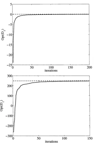
2.4 The projection vector W obtained with sparseness constraints (-) = 3 (left) and no sparseness constraints (right). Clearly the sparseness constraints do produce a sparse W while most of U s elements are active without sparseness constraints... 36 3.1 The objective value of the dual problem (I)i) on the first (top) and

C h a p ter 1

Introd u ction

In this chapter, we present an overview of metric learning and convex

optimization. Most relevant work to our algorithms will be given in each chapter. Here we focus on a brief introduction to general metric methods. We also provide fundamental backgrounds on convex optimization, in particular, linear

programming and semidefinite programming.

1.1

D is ta n c e M e tr ic L ea rn in g

Many classical machine learning algorithms, such as k-nearest neighbor (A’-NN), usually rely upon the distance metric over the input data vectors. Distance Metric learning is to learn a distance metric for the input space of data, from a. set of pair of similar/dissimilar points that preserves the distance relation among the training data. Previous work has demonstrated that a learned metric can indeed greatly improve the performance in classification, clustering and other learning tasks [53, 31, 12, 15, 41. 22. 48. 42].

imsupervised metric learning and supervised metric learning. For example,

principal component analysis (PCA) and multidimensional scaling (MDS) that do not utilize any label information are unsupervised learning. In this thesis, we mainly focus on supervised learning for classification; i.e., learning a distance metric from side information that is usually presented in a set of pairwise (or distance comparison) constraints. The optimal distance metric is typically sought by preserving these constraints and at the same time, optimizing a certain

regularized term.

In the following, we will review a few classical methods and those mostly related to ours. Spectral methods are a class of traditional algorithms used to discover informative linear projections of the input space. The linear projections can be viewed as learning Mahalanobis distance metrics. Note that typically the learned Mahalanobis metrics are rank deficient in this case. We review some widely-used spectral methods here. These linear methods can usually be kemelized using the kernel trick. The kernel versions of these methods are beyond the scope of this thesis.

Principal component analysis and linear discriminant analysis (LDA) are two classical dimensionality reduction techniques. PCA finds the subspace that has maximum variance of (lie input data. LDA tries to project the data onto a subspace by maximizing the between-class distance and minimizing the

wit hin-class variance. Essentially both methods compute the linear transformation P such that the original data x are projected to a low-dimensional space by PTx. The covariance matrix of the input data can be written as

1 N

C = — ^ 2 { x?. - fi)(xi - n)T , (1.1) i—1

orthogonal. Mathematically it is

m a x T r(P T C P ), subject to PT P = I (1.2)

This problem can be solved by eigen-decomposition of C. As discussed, PCA does not use any class label information and it is an unsupervised method. In practice, PCA can be used to pre-process the input data, li has some de-noise functionality. By only keeping a few top eigenvectors of the decomposition, PCA projects the data into a low-dimensional space and thus reduces the computational complexity. In contrast, LDA finds the linear projection matrix P that maximizes the

between-class variance and at the same time minimizes the within-class variance. If Sw and Sf, denote the within-class scatter matrix and between-class matrix respectively, the optimization problem we want to solve is

max Tr ((P TSWP ) ~ \ P T Sbp f ) , subject to PT P = I. (1.3)

This problem can again be solved using generalized eigen-decomposition [23]. LDA has been widely used in many application due to its simplicity and effectiveness. There are many other variants of LDA. for example [52, 27]. In some scenarios, these variants perform better than LDA.

Until recently, work has been done on learning a metric using the pairwise

constraints (a.k.a., equivalence constraints), which are formed bv the relationship of pairs of data. Given two training points x, and Xj, if they belong to the same class, we ought to minimize the distance between x% and X j; otherwise we maximize their distance. In the context of learning a Mahalanobis distance, the problem can be written as

Here sets S and V denotes the similarity set and dissimilarity set respectively. Note that the positive semidefiniteness constraint A' )? 0 is needed to ensure a valid Mahalanobis matrix. \\xi — ccy| | ^ = (x } — Xj)TX ( x i — Xj) is the distance between x, and x t with the Mahalanobis metric matrix X . The relationship between the Mahalanobis metric matrix X and the linear projection matrix P is:

A = P P T .

This is why methods like1 PCA or LDA can be viewed as metric learning

algorithms. (1.4) always produces a rank-one solution [48]. To avoid this problem, the first constraint in (1.4) is changed to YhXi X)e v \J\\x i ~ x j llx — ^ 'n [48].

Although the resulting problem is a convex program and hence the global

optimum is guaranteed, it may not be trivial to solve. It is in a general form and the semidefiniteness constraint makes (he problem not scale well. (1.4) was advocated to improve the performance of clustering algorithms like A'-ineans. It may not be appropriate for learning a distance metric for A--NN classification. Neighborhood component analysis (NCA) is proposed to learn a Mahalanobis distance for A’-NN classification bv minimizing the leave-one-out error [18]. Given a training point Xj, the probability that x, being a. neighbor of X{ is ptj :

exp( —||PT Xj — PTXj\\2)

>lJ E f c ^ e x P H I ^ T ®i “ p T x kII2 ) '

large number of training data, or the dimensionality of the data is high. NCA does not scale well because the number of parameters in the projection matrix is

quadratic in the dimensionality. It becomes computationally intractable when the dimensionality is large.

A related algorithm, termed metric learning by collapsing classes (MLCC). was proposed in [17]. Unlike NCA, MLCC can be formulated as a convex optimization over the space of positive semidefinite matrices. A drawback of MLCC is that it implicitly assumes that the data points in each class have a unimodal distribution such that they can be collapsed to a single point in the transformed space.

In [46], a large margin nearest neighbor method is designed to learn a Mahalanobis metric. The goal is to make t he /.’-nearest neighbors always belong to the same class while examples from different classes are separated bv a large margin. As in support vector machines, the margin criterion leads to a convex optimization using the hinge loss. It can handle multi-class problems naturally. The problem is formulated as a standard semidefinite program, which can be solved using off-the-shelf solvers like SeDemi [43], CSDP [5], or SDPT3 [45].

Given th at convex optimization becomes more and more important in machine learning and recent advances in metric learning have proved its usefulness, we review some fundamental concepts here. In part icular, we give an overview of linear programming and semidefinite programming, which arc our tools for the algorithms developed in the next two sections.

1.2

C o n v e x O p tim iz a tio n

A mathematical programming problem has the form

min fo(x)

The variable to be optimized is a. vector x. /o is the objective function and fj. i = 1. • • • , m, are the constraints. When all the functions involved in (1.6) are convex, the program is a special case, for which the global optimum is usually able to be efficiently found (in polynomial time). This class of problems is generally referred to as convex optimization problems. There is in general no analytical formula for the solution of convex optimization problems. However, there are effective methods for solving some special cases. The interior-point method is one of the methods [6]. We focus on two special cases of (1.6) here, namely linear programs and semidefinite programs.

1.2.1 L inear p ro g ra m m in g

In this section, we overview techniques of linear programs (LP). LP has a, linear objective function, and a. bunch of linear equality and linear inequality constraints. The st andard form of LP writes:

max cT x

s.t. Ax < b. (1.7)

x is the vector of variables and c and b are vectors of known coefficients and the matrix A is also known. Many practical problems in operations research can be expressed as LPs.

Given an LP. referred to as a primal problem, there is a corresponding dual problem, which provides an upper bound to the optimal value of the primal problem. In matrix form, we can express the primal problem as:

max cTx

The corresponding dual problem is

min b] y

s.t. A1 y > c. y > 0. (1.9)

where y is the dual variable.

The duality theory states that (1) the dual of a dual LP is the original primal LP; (2) Every feasible solution for an LP gives a bound on the optimal value of the objective function of its dual; (3) The strong duality theorem states the optimum of the dual and the optimum of the primal coincide. Therefore one can always solve an LP by solving its dual. See [6] for details about the weak and strong duality theorems and their conditions.

There are two main algorithms for solving LPs: simplex and interior point algorithms. The simplex algorithm solves LP problems by constructing an

admissible solution at a vertex of the polyhedron and then walking along edges of the polyhedron to vertices with successively higher values of the objective function until the optimum is reached. The simplex method is usually fast in practice. However, the theoretical worst complexity is exponential time. In contrast, interior point methods finds the optimal solution by progressing along points on the boundary of a polyhedral set. Interior point methods start from the interior of the feasible region and converge to a vertex. There are many efficient off-the-self LP solvers, c.g., CPlex [26], Mosek [34]. CPlex can solve large-scale problems up to

10(’ variables and constraints.

1.2 .2 S e m id efin ite p ro g ra m m in g

semidefinite cone. In general, an SDP has the form:

min (C. X)

s.t. (Ai, X) = bi,i = 1. • • • . ra, (1.10)

X 'rp 0.

The variable we want to optimize is X. Here (A. B) = Yl rj AjjBjj calculates the inner product of two matrices.

We can also derive its dual problem as in the case of LP.

max (b. y)

m

s.t.

y^

yjAj ^

c.

(1.11)

i=1

The dual variable is y. Here A =<! B means A — B ^ 0 or B — A 0. Like LP, the weak duality and strong duality hold for SDPs under some

conditions. Usually the weak duality always holds even for non-convex problems. The weak duality can be used to find nontrivial lower bounds for difficult

problems. The strong duality usually holds for convex problems. The conditions that guarantee strong duality in convex problems are called constraint

qualifications. See [6] for details. Unlike LP where one can always recover the primal solution from the dual solution by solving a linear system, one may not always be able to find the primal solution of an SDP from its dual. However, interior point methods solve the primal and dual at the same time.

as metric learning and kernel learning, can be formulated as SDPs. The desirable properties of these formulations are: (1) The global optimum is guaranteed. In other words, it is local-optimum-free; (2) For reasonable-scale problems (up to a few thousand variables), interior point methods work efficiently. Nevertheless, as mentioned before, current solvers do not scale very well, largely due to an inverse of the Hessian matrix needs to be calculated and stored, which requires cubic complexity. It is an active research topic to design first-order methods for solving SDPs. in which no Hessian is involved [6].

C hapter 2

Supervised D im en sion ality

R ed u ction via Sequential S D P

Many dimensionality reduction problems end np with a trace quotient formulation, for example, the linear discriminant analysis method. Since it is difficult to

directly solve the trace quotient problem, traditionally the trace quotient cost function is replaced by an approximation such that generalized

eigen-decomposition can be applied. By contrast, we directly optimize the trace quotient in this work. It is reformulated as a quasi-linear semidefinite optimization problem, which can be solved globally and efficiently using standard off-the-shelf semidefinite programming solvers. Also this optimization strategy allows one to enforce additional constraints (for example, sparseness constraints) on the projection matrix. We apply this optimization framework to a novel

dimensionality reduction algorithm. The performance of the proposed algorithm is demonstrated in experiments on several UCI machine learning benchmark

2.1

I n tr o d u c tio n

In pattern recognition and com puter vision, techniques for dimensionality reduction have been extensively studied [44, 46. 48, 42. 49]. Many of the

dimensionality reduction methods, such as linear discriminant analysis (LDA) and its kernel version, end up with solving a trace quotient problem

W° argmax

wTw=ldxd

T r ( W J S bW)

T r ( ll/T.S',,I4/ ) ’ (2.1)

where S b, S v are two positive semidefinite (p.s.d.) matrices (Sb 0, S v ^ 0), I the d x d identity m atrix (sometimes the dimension of I is om itted when it can be inferred from the context) and Tr(-) denoting th e m atrix trace. W G Wnxd is target projection m atrix for dimensionality reduction (typically d D). In the supervised learning framework, usually S b represents the distance of different classes while Sv is the distance between d ata points in the same class. For

example. Sb is the inter-class scatter matrix and S v is the intra-class scatter m atrix for LDA. By formulating the problem of dimensionality reduction in a general setting and constructing S b and S v in different ways, we can implement many different m ethods in the above m athem atical framework.

Despite the im portance of the trace quotient problem, to date it lacks a direct and globally optim al solution. Usually, as an approximation, the quotient trace cost T r((lF TS VW) 1 (W’TSbW)) is instead used such th a t the generalized

of S~1 Sb corresponding to the largest eigenvalues are used to form the optimal W°. It is believed that the largest eigenvalue contains more useful information. Nevertheless such a GEVD approach cannot produce an optimal solution to the original optimization problem (2.1) [49]. Furthermore, the GEVD approach does not yield an orthogonal projection matrix. It is shown in [8. 25] that orthogonal basis functions preserve the metric structure of the data better and they have more discriminating power. Orthogonal LDA (OLI)A) is proposed to compute a set of orthogonal discriminant vectors via the simultaneous diagonalization of the scatter matrices [52]. In [51] it is shown that solely optimizing the Fisher criterion does not necessarily yield optimal discriminant vectors. It is better to include correlation constraints into optimization. The features produced by the classical LDA could be highly correlated (because they are not orthogonal), leading to high redundancy of information. Including correlation constraints such as

H't(S„ + Sb)W = 0

could be beneficial for classification [51].

Recently semidefinite programming (SDP) or more general convex programming [6, 3] has been attracting more and more interests in machine learning due to its flexibility and desirable global optimality [47. 28. 31]. Moreover, there exist interior-point algorithms to efficiently solve SDPs in polynomial time. Large margin nearest neighbor (LMNN) [46] is an example of using SDP to learn a metric. LMNN learns a metric by maintaining consistency in d ata’s neighborhood and keeping a large margin at the boundaries of different classes. It has been shown in [46] th at LMNN delivers the state-of-the-art performance among most distance metric learning algorithms.

• The low target dimension is selected by the user and the algorithm guarantees a globally optimal solution using fractional programming. In other words, it is local-optima-free. Moreover, the fractional programming can be efficiently solved by a sequence of SDPs;

• The projection matrix is orthonormal naturally;

• Unlike the GEVD approach to Id)A. using our proposed algorithm, the data are not restricted to be projected to at most c — 1 dimensions. Here c is the number of classes.

To our knowledge, this is the first attem pt th at directly solves the trace quotient problem and meanwhile, a global optimum is deterministically guaranteed. We then develop methods to design Sb and Sv. The traditional LDA is only optimal when all the classes follow single Gaussian distributions that share the same covariance matrix. Our new Sb and Sv are not confined by this assumption. The remaining content is organized as follows. In Section 2.2, we describe our algorithm in detail. Section 2.3 applies this optimization framework to

dimensionality reduction. In Section 2.4. we briefly review relevant work in the literature. The experiment results are presented in Section 2.5. We discuss new extensions in Section 2.6. Finally concluding remarks are discussed in Section 2.7.

2.2

Solving th e T race Q u o tie n t P ro b le m U sing S D P

2.2.1 S D P f o r m u la tio n

By introducing an auxiliary variable S, the problem (2.1) is equivalent to

maximize

6,W 4' (2.2a)

subject to T r(WTS bW) > S ■ Tr{WTS vW) (2.2b)

X

II _(2.2c)

W £ R Dxd. (2.2d)

The variables we want to optimize here are 5 and W. But we are only interested in W with which the value of ri is maximized. This problem is clearly not convex because the constraint (2.2b) is not convex, and in addition (2.2d) is actually a non-convex rank constraint. (2.2c) is quadratic in W . It is obvious that must be positive.

Let us define a new variable Z £ EI)xD. Z - W W T , and now the constraint (2.2b) is converted to Tv((Sb — SSV)Z) > 0 under the fact that

Tr(H/T5H ) = TV(.S'U'U' ) = T r(SZ). Because Z is a matrix production of W and its transpose, it must be p.s.d. In terms of Z, the cost function (2.1) is a linear fraction, therefore it is quasi-convex (More precisely, it is also quasi-concave, hence quasi-linear [6]). The standard technique for solving quasi-concave maximization (or quasi-convex minimization) problems is bisection search which involves solving a sequence of SDPs for our problem. The following theorem due to [36] serves as a basis for converting the non-convex constraint (2.2d) into a linear one.

T h e o re m 2.2.1. Define sets P i = { W W T : WT W = Idxd} and

P 2 = {Z : Z = Z r , T r (Z) — d. 0 Z =<( I}. Then P i is the set of extreme points of P 2.

il‘2- Therefore constraints (2.2c) and (2.2d) can he relaxed into Tr(Z) = d and 0 ^ Z ^ I, which are both convex. When the cost function is linear and it is subject to S2‘2. the solution will be at one of the extreme points [37]. Consequently, for linear cost functions, the optimization problems subject to Qi and ilo are exactly equivalent.

With respect to Z and 6, (2.2b) is still lion-convex: the problem may have locally optimal points. But still the global optimum can be efficiently computed via a sequence of convex feasibility problems. By observing that the constraint is linear if 5 is known, we can convert the optimization problem into a. set of convex feasibility problems. A bisection search strategy is adopted to find the optimal S. This technique is widely used in fractional programming [6. 1]. Let denote the unknown optimal value of the cost function. Given 6* £ K. if the convex feasibility problem1

find Z (2.3a)

subject to Tr ((Sb — 6*SV)Z) > 0 (2.3b)

Tr(Z ) = d (2.3c)

0 ^ Z =<: I (2.3d)

is feasible, then we have 3° >3*. Otherwise, if the above problem is infeasible, then we can conclude 3° < 3*. This way we can check whether the optimal value 3° is smaller or larger than a given value 3*. This observation motivates a simple algorithm for solving the fractional optimization problems using bisection search, which solves an SDP feasibility problem at each step. Algorithm 1 shows how it works.

Thus far, a. question remains unanswered: are constraints (2.3c) and (2.3d)

A lg o rith m 1 Bisection search.

R eq u ire: 5/: Lower bounds of S\ fi„: Upper bound of <5 and the tolerance a > 0. w hile Slt — ()/ > ct do

* _ Si+6tl

u 2

Solve the convex feasibility problem described in (2.3a)-(2.3d). if feasible th e n

Si = 6; else

Su = s . e n d if e n d w hile

equivalent to constraints (2.2c) and (2.2d) for the feasibility problem? Essentially the feasibility problem is equivalent to

maximize Tr!(Sk - S ' S V)Z) (2.4a)

subject to Tr(Z ) = d (2.4b)

o =<; Z I. (2.4c)

If the maximum value of the cost function is non-negative, then the feasibility problem is feasible. Conversely, it is infeasible. Because this cost function is linear, we know that can be replaced bv SU, i.e., constraints (2.3c) and (2.3d) are equivalent to (2.2c) and (2.2d) for the optimization problem.

Note that constraint (2.3d) is not in the standard form of SDP. It can be rewritten into the standard form as

Z 0 0 Q

^ 0.

Z + Q = I,

(2.5a)

(2.5b)

our experiments.

2 .2 .2 E stim a tin g b o u n d s o f

5

The bisection search procedure requires a low bound and an upper bound of <5. The following theorem from [36] is useful for estimating the bounds.

Theorem 2.2.2. Let S € D he a symmetric matrix, and

(fS.i > <Ps,2 > • • * > ‘rs.D he the sorted eigenvalues o f S from largest to smallest.

then

d max TV(W'tSW0 = V W

WTW = l dxd “

Refer to [36] for the proof. This theorem can be extended to obtain the following corollary (following the proof for Theorem 2.2.2):

Corollary 2.2.1. Let S £ M.°xr) he a symmetric matrix, and

ips,

1 <

ips

,2 < • • • <

ips.D

b e its sorted eigenvalues from smallest to largest, then

d min rIV(IT S\V) = V ^ S i.

VVT W = l dxd “

Therefore, we estimate the upper bound of ():

s u =

g r

1

—

(2-6)

z2z=\ v>sv,i

In the trace quotient problem, both Sb and S v are p.s.d. That is to say, all of their eigenvalues are non-negative. Be aware that the denominator of (2.6) could be zeros and fiu = +oc. This occurs when the d smallest eigenvalues of S v are all zeros. In this case, rank(5v) < D — d. In the case of LDA,

A principle component analysis (PCA) preprocessing can always be performed to remove the null space of the covariance matrix of the data, such that Su becomes valid.

A lower bound of h is then

Si = ll-Sh.i l ^ i =1VSr.i

(2.7) Clearly S[ > 0.

The bisection algorithm converges in [log2( <)~"~^)] iterations, and obtains the global minimum within the predefined accuracy of cr. The bisection procedure is intuitive to understand. Next we describe another algorithm Dinkelbach's algorithm less intuitive but faster, for fractional programming.

2.2.3 Dinkelbach’s algorithm

Dinkelbach algorithm [39] proposes an iterative procedure for solving the fractional program maximize® f ( x) / g( x) , where x is constrained on a convex set and f ( x) is concave, g{x) is convex. It considers the parametric problem.

maximize® f { x) — Sg(x),

where S is a constant. Here we need to solve

maximize^ Tr((5)> — 6SV)Z). (2.8)

The algorithm generates a sequence of values of S's that converge to the global optimum function value. The bisection search converges linearly while the Dinkelbach’s algorithm converges super-linearly (better than linearly and worse than quadratically).

A lg o rith m 2 Dinkelbach algorithm.

R eq u ire: An initialization Z ((,) which satisfies constraints (2.4b) and (2.4c). Set

Tr(S^(»)) Tr(SvZ<°>)

and k = 0.

(★ ) k = k 4-1. Solve the SDP (2.8) subject to constraints (2.4b) and (2.4c) to get. the optimal Z ik\ given 6.

if T r((Sb - 6SV) Z W) = 0 th e n stop and the optimal Z° = Z^k\ else

Set

A _ T r(ShZ ^ ) T r (S„Z<*)) and go to step (*).

e n d if

found in [39]. In Algorithm 2. note that: (1) A test of the form Tr((S'fe — ÖSv) Z (-k'1) > 0 is unnecessary since for any fixed k,

T r((Sb - &SV)ZW) = maxz T r((Sb - SSV) Z) > Tr( ( Sb - 6SV) Z(k~V) = 0. However due to computer's numerical accuracy limit, in implementation it is possible that the value of T r ((Sb — 5SV) Z ^ ) is a negative value which is very close to zero; (2) To find the initialization Z^(,) that must reside in the set defined by the

2 .2 .4 C o m p u tin g

W

from Z

From the covariance matrix Z learned by SDP. we can calculate the projection matrix W by eigen-decomposition. Let Vj denote the ifh eigenvector, with eigenvalue Xt. Let Ai > A2 > • • • > Xd be the sorted eigenvalues. It is

straightforward to see that W = diag(\/Ai, \f^2~ • • • , \/Xd) VT, where diag(-) is a square matrix with the input as its diagonal elements. To obtain a D x d

projection matrix, the smallest I) — d eigenvalues are simply truncated. The projection matrix obtained in this wav is not the same as the projection corresponding to maximizing the cost function subject to a rank constraint. However this approach is a reasonable approximation. Moreover, like PC A. dropping the eigenvectors corresponding to small eigenvalues may de-noise the input data, which is desirable in some cases.

This is the general treatment for recovering a low dimensional projection from a. covariance matrix. In our case, this procedure is precise. This is obvious: A;, the eigenvalues of Z = W WT, are the same as the eigenvalues of WTW = Idxd- That means, Ai = A2 = • • • = A<* = 1 and the remaining D — d eigenvalues are all zeros. Hence in our case we can simply stack the first d leading eigenvectors to obtain W.

2 .3

A p p lic a ti o n t o D im e n s io n a lity R e d u c t i o n

There are various strategies to construct the matrix Sb and Sv, which represent the inter-class and intra-class scatter matrices respectively. I11 general, we have a set of data { xp} *^ € R n and we are given a similarity set S and a dissimilarity set V. Formally, {S : (x p, x q) € S if x p and x q are similar} and

{ V : (xp, x q) G V if x p and x q are dissimilar}. We want to maximize the distance

dist w ( x p, x q) = \\WTX p - W T X q \\2

©

o

# O are different classes

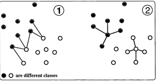
Figure 2.1: The connected edges in (1) define the dissimilarity set V and the con­ nections in (2) define the similarity set S. As shown in (1), the inter-class marginal samples are connected while in (2). each sample is connected to its k' nearest neigh­ bors in the same class. For clarity only few connections are shown.

where St, =

Y2(p

q)eT>(x p ~~ x q)(x p ~~ x q)' • This distance measures the inter-class distance. We also want to minimize the intra-class compactness distance:

Inspired by the marginal fisher analysis (MFA) algorithm proposed in [50], we construct similar graphs for building Sb and Sv. Figure 2.1 demonstrates the basic idea. For each class, assuming x p is in this class, and if the pair (p, q) belongs to the k closest pairs that have different labels, then (p. q) V. The intra-class set S is easier: we connect each sample to its k' nearest neighbors in the same class, k and k! are parameters defined by the user.

(p,q)eT>

Tr (SbZ)

Y . d is t\y(xp, X q ) = Tl' (SVZ )

(p.q)eS

[image:34.526.140.397.99.235.2]

This strategy avoids certain drawbacks of LDA. We do not force all the pairwise samples in the same class to be close (This might be a too strict requirement). Instead, we are more interest in driving neighboring samples as closely as possible. We do not assume any special distribution on the data. The set V characterizes the margin information between classes. For non-Gaussian data, it is expected to better represent the separability of different classes than the inter-class covariance of LDA. Therefore we maximize the margins while condensing individual classes simultaneously. For ease of presentation, we refer this algorithm as SDPi, whose Sb and Sv are calculated by the above-mentioned strategy.

[16] defines a 1-nearest-neighbor margin based on the concept of the nearest neighbor to a point x with the same and different label. Motivated by their work, we can slightly modify MFA's inter-class distance graph. The similarity set S remains unchanged as described previously. But to create the dissimilarity set V. a. simpler way is that, for each x p we connect it to its k differently-labeled neighbors a y s (x p and x q have different labels). The algorithm that implements this concept is referred to as SDP2. It is difficult to analyse which one is better. Indeed the

experiments indicate for different data sets, no single method is consistently better than the other one. One may also use support vector machines (SVMs) to find the boundary points of the separation plane and then create T> (and then Sb) based on those boundary points [15].

2 .4

R e l a t e d W o r k

The closest work to ours is [49] in the sense that it also proposes a method to solve the trace quotient directly. [49] finds the projection matrix W in the Grassmann manifold. Compared with optimization in the Euclidean space, the main

method: (1) [49] optimizes Tr(U T S^W — 4 • W TSVW) and they do not have a principled way to determine the optimal value of 4. In contrast, we optimizes the trace quotient function itself and a deterministic bisection search or the

Dinkelbach's iteration guarantees the optimal 4: (2) The optimization in [49] is non-convex (difference of two quadratic functions). Therefore it is likely to become trapped into a local maximum, while our method is globally optimal.

[32] simply replaces LDA’s cost function with T r ( W TS^W — W TSVW), i.e., setting 4 = 1. Then GEVD is used to obtain the low rank projection matrix. Obviously this optimization is not equivalent to the original problem, although it avoids the matrix inversion problem of LDA.

[48] proposes a convex programming approach to maximize the distances between classes and simultaneously to clip (but not to minimize) the distances within classes. Unlike our method, in their approach the rank constraint is not considered. Hence it is metric learning but not necessary a dimensionality reduction method. Furthermore, although the formulation of [48] is convex, it is not an SDP. It is more computationally expensive to solve and general-purpose SDP solvers are not applicable. SDP (or general convex programming) is also used in [46. 17] for learning a distance metric. [46] learns a metric th at shrinks distances of neighboring similarly-labeled points and repels points in different classes bv a large margin. [17] also learns a metric using convex programming.

2.5

E x p e r im e n ts

In mH our experiments, the Bisection Algorithm 1 and Dinkelbach's Algorithm 2

output almost identical results but Dinkelbach converges as twice faster as Bisection does.

We observe that the direct solution indeed yields larger trace quotient than the quotient trace using GEVI) because that is what we maximize.

D a ta v isu alizatio n . As an intuitive demonstration, we run the proposed SDP algorithms on an artificial concentric circles data set [18]. which consists of four classes (shown in different colors). The first two dimensions follow concentric circles while the remaining eight dimensions are all Gaussian noise. When the scale of the noise is large, PGA is distracted by the noise. LDA also fails because the data set is not linearly separable and each class' center overlaps in the same point. Both of our algorithms find the informative features (Figure 2.2-(3)(4)). Ideally we should optimize the projected neighborhood relationship as in [18]. Unfortunately it is difficult. [18] utilizes soft max nearest neighbors to model the neighborhood relationships before the projection is known. However the cost is non-convex. As an approximation, one usually calculates the neighborhood relationships in the input space. Laplaeian eigenmap [2] is an example. ? noise is large enough, the neighborhood obtained in this way may not faithfully represent t he true data structure. We deliberately set the noise of the concentric data set very large, which breaks our algorithms (Figure 2.2-(5)(6)). Nevertheless useful prior information can be used to define a meaningful V and S whenever it is available. As an example, we use the sets T> and S of Figure 2.2-(3)(4) and then calculate Sb and Sv with the highly noisy data, our algorithms are still able to find the first two useful dimensions perfectly, as shown in Figure 2.2-(7)(8).

neighbor classifier (LMNN)2. Note th at our algorithm is much faster than LMNN in [46]. especially when the number of training data is large. That is because the complexity of our algorithm is independent of t he number of data while in [46] more data produce more SDP constraints that sknv down the SDP solver. A description of the data sets is in Table 2.1.

PC A is used to reduce the dimensionality of image data (USPS handwritten digits'5 and ORL face data4) as a preprocessing procedure for accelerating the computation. For five data sets the results are reported over 50 random 70/30 splits of the data. USPS has a predefined training and testing sets.

In the experiments, we did not carefully tune the parameters (k,k') associated with our proposed SDP approaches due to computational burden. However, we find that the parameters are not sensitive in a wide range. They can be optimally determined by cross-validation. We report a 3-NN (nearest neighbor) classifier’s testing error. The result is shown in Table 2.2. where the baseline is obtained bv directly apply 3-NN classification on the original data. Next we present details of tests.

UCI data sets: Iri. Wine and Bal. These are small data sets with only 3 classes, which are from UCI machine learning repository [35]. Except the Wine data, which are well separated and LDA performs best, for the other two data, our SDP algorithms present competitive results.

USPS digit recognition. Two tests are conducted on the USPS handwriting digit data set. In the first test, we use all the 10 digits. USPS has predefined training and testing subsets. The training subset has 7291 digits. We randomly split the training subset: 20% for training and 80% for testing. The dimensionality of these

16 x 16 images are reduced to 551) by PCA. 90.14% of the variance is preserved.

" The codes are obtained from the au th ors’ website h t t p : //www. w e in b e r g e r w e b . n e t / D o w n lo a d s / LMNN. html

’h t t p : //www. g a u s s i a n p r o c e s s . o r g / g p m l / d a t a /

0 R L 2 2 0 0 2 0 0 4 0 6 4 4 4 2 (2 0 0 ,3 ) (2 .3 ) 5 0 —: C 2 8 0 1 2 0 4 0 6 4 4 4 2 (3 0 0 .3 ) (2 .3 ) 5 0 U S P S

2 l, ^_N

77 00 50 n - lO

S C M CO to 3 o - t-H

^ cc <N 10 = d

U S P S 1 1 4 5 9 5 8 3 2 1 0 2 5 6 5 5 (3 0 0 .3 ) (3 ,5 ) 10 B a l 4 3 8 1 8 7

3 4 4

(2 2 0 .3 ) (3 .5 ) 5 0 W in e

§ SI « 2 2 § 2 3

—1 IO d

Ir

is o ^ CO ^ ^ O £ g

—H

LMNN gives the best result with an error rate 4.22%. Our SDPs have similar performance. For the second test, it is only run once with the predefined training subset and test subset. The digits 1.2 and 3 are used. On this data set. our two SDPs deliver lowest test errors. It is worth noting that LDA performs even worse than PCA. This is likely due to the d ata’s non-Gaussian distribution.

ORL face recognition. This data set consists of 400 faces of 40 individuals: 10 per each. The image size is 5G x 46. We down-sample them by a factor of 2. Then PCA is applied to obtain 42D eigenfaces. which captures about 81%> of the

variance. Again two tests are conducted on this set. The training and testing sets are obtained by 7/3 and 5/5 sampling for each person respectively. For both tests, LMNN performs best, and SDPj is the second best one. Also note that for each method, its performance on OH LI is better than its corresponding result on ORL2. This is expected since OH Li contains more training examples.

For all the tests, our algorithms are consistently better than PCA and LDA. The state-of-the-art LMNN outperforms ours on tasks with many classes such as USPS1, ORLl and ORL2. It might be due to the fact that, inspired bv SVM, LMNN enforces constraints on each training point. These constraints ensure that the learned metric correctly classifies as many training points as possible. The price is that LMNN's SDP optimization problem involves many constraints. With a large amount of training data, the required computat ional demand could be prohibitive. This is because the number of variables of LMNN is linear in the number of training data points. Therefore as SVM, it is difficult to scale it to large size problems. In contrast, our SDP formulation is independent of the amount of training data. The complexity is entirely determined by the dimension of the input data.

more experiments. We run SDPs and LMNN on the data set ORL2. We vary the number of classes c from 5 to 32. The first c individuals’ images are used. The parameters of SDP2 remain unchanged: k = 2 and k' = 3. For each value of c, the experiment is run 10 times. We report the classification result in Table 2.3. This result confirms that our SDPs perform well for tasks with few classes. It also explains why LMNN outperforms our SDPs for data sets having many classes. It might also be possible to include constraints as LMNN does in our SDP

formulation.

The second classification experiment we have conducted is to compare our methods with two LDA's variations, namely, uncorrelated linear discriminant analysis (ULDA) [27] and orthogonal linear discriminant analysis (OLDA) [52]. ULDA was proposed for extracting feature vectors with uncorrelated attributes. The crucial property of OLDA is that the discriminant vectors of OLDA are orthogonal to each other (In other words, the transformation matrix of OLDA is orthogonal). The Yale face database5 is used here. The Yale database contains 165 grav-scale images of 15 individuals. There are 11 images per subject. The images

demonstrate variations in lighting condition, facial expression (normal, happy, sad. sleepy, surprised, and wink). The face images are manually aligned and cropped into 32 x 32 pixels, with 256 gray levels per pixel. The 11 faces for each individual is randomly split into training and testing sets by 4/7. 5/6 and 6/5 sampling. PC A is performed to reduce 1024D into 50D. which contains above 98% of the total variation.

An important parameter for most subspace learning based face recognition

methods is dimensionality estimation. Usually the classification accuracy varies in the number of dimensions. Cross validation is often needed to estimate the best dimensionality. We simply set the dimensionality to c — 1, where c is the number

O R L 2 8.68( 2. 01 ), 4 2 7. 63( 1. 93) , 3 9 4 .6 9 (1 .9 8 ). 4 2 6.64(2 .21 ), 3 9 5 .8 7 (1 .9 8 ). 3 9 0RL 1 5.1 1(1 .91 ), 42 4. 85( 1. 92) , 3 9 2 .2 3 (1 .3 9 ), 4 2 3. 47( 1. 56) , 3 9 3. 3 2 (1 .2 4 ). 3 9 U S P S 2

2.39.256 2.0

7 . 5 0 3 .0 3 . 2

1.91,50 1.7

5 .4 0 1 .9 1 .4 0 U S P S 1 6 .36 (0 .2 1). 2 5 6 5.6 0 (0 .2 7 ). 55 7 .4 3( 0. 4 2 ), 9 4 .2 2 (0 .3 5 ), 5 5 5 .28 (0 .2 5), 5 0 4 .7 3 (0 .1 0 ), 5 0 B a l

f ^ n ” 3 3 „

s—v V, V /- N

S I S » S g

c4 H

O 2 2, - 22 o' 00 <N CO N 00 *7

—^ y— i y—^ rH i—H

W

in

e

” » (N ” x

0 0 CO CCT 57 ^ 7;

7 ® a o £ “ " JfL - =4 5 ifL 22 22

ci os ^ 9 _{M H ^ i 1} *> c i_h

I Ir is 4.57( 2. 50 ). 4 4 .80 (2 .5 1). 2 4.23( 2. 56 ), 2 4.40 (2 .75 ), 4 3 .0 2 (2 .1 9 ). 3 3 .6 0 (2 .6 1 ), 3 b as el in e P C A L D A L M N N S D P i s d p 2

In J5

I - s

a; ö S I 'S -3 o 1 a

2 I

Li

_<M — CO 2 a- 5 co u

& 's 0 53 O ">J X -M ^ s

1 1 3 H

33 -Ö Si_O 1 6

0 O - ^3 3 C 1

1 i u O Z ^ Z .2 cc ^3

35

M

■___, 4_^

2 1

£ -S

0 eg - 0>

1 Ö

_{4_2 «-4—I}

33 ^ u S

<S .2

* S X1 33 Ü

6 J

3 2 3 .1 2 (2 .0 5 ) 4.63(1.36) 25 2 .3 4 (1 .3 8 ) 3.20( 1.77) oc 3.4 9( 2. 08) 3 .1 1 (1 .7 2 ) r-—< 1 .5 7 (1 .6 0 ) 1 .2 9 (1 .0 5 ) 2 3 .8 0 (1 .9 9 ) 1 .2 0 (1 .2 0 ) 00 5.0 0 (3 .3 3 ) 0 .1 3 (0 .5 6 ) IO 0 (0 ) 0 (0 ) 8 1 CJ u _ %

Z\ Ol

Z

3-1—1 o Ö te_o 'S | o II O ä ÜH o ■u ö o T j z T m-i jH S X > s I_o z z CO <+H • X 1 'S c3 ^ r \

3 3 'S f-) o J-H 1) bO »—i "35 55 aj o .3 £ .2 J u s I z z <—I <5 2 I 'S xd jd To I .2 Ch Q cd 1 O bO T Cu Q cd 2 Ö

1 £_{ec x} r ^ uX .2

1

r->

•g_£

"ö Q, ■s I

55 tö H3

5 a I ° o a pJ a3

«2 2 cö .2 rO

O pH

a 1

-2 •-To .'S

2 Z

s s

of classes. That means, on the Yale dataset, the final dimensions for all algorithms are 14. As in the first experiment, we also fix the parameters of SDPo: k = 2 and k! = 3.

4 Train 5 Train 6 Train

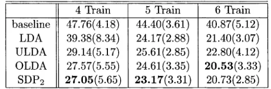
baseline 47.76(4.18) 44.40(3.61) 40.87(5.12) LDA 39.38(8.34) 24.17(2.88) 21.40(3.07) ULDA 29.14(5.17) 25.61(2.85) 22.80(4.12) OLDA 27.57(5.55) 24.61(3.35) 20.53(3.33) S1)P2 27.05(5.65) 23.17(3.31) 20.73(2.85)

Table 2.4: Classification error of a 3-NN classifier on the Yale face database in the format of m ean (std )% . Each case is run 20 times to calculate the mean and standard deviation. SDP2 performs slightly better than OLDA.

Table 2.4 summarizes the classification results. We see that ULDA performs similarly with the traditional LDA. OLDA achieves higher accuracies than ULDA and LDA. The proposed SDP algorithm is slightly better than OLDA. Since both OLDA and the proposed SDP algorithm produces orthogonal transformation matrix, we may conclude that orthogonality does benefit subspace based face recognition.

As mentioned, for the LDA algorithm and its variations, the data are restricted to be mapped to at most c — 1 dimensions. Our SDP algorithms do not have this restriction. We have compared the final classification results on Yale when the final dimensionality varies using the SDP2 algorithm in Table 2.5. It can be observed that c — 1 is not the best dimensionality for SDP2 in this case.

final dimensions 14 20 24 30

s d p2 27.05(5.65) 26.43(5.14) 26.86(4.18) 28.62(5.27) Table 2.5: Classification error of a 3-NN classifier on the Yale face database with 4 training examples. Each case is run 20 times.

[image:44.526.134.399.161.248.2]

algorithm needs around 80 seconds to converge. In contrast, LDA, ULDA or OLD A needs about 2 seconds6.

2.6

E x te n s io n : E x p lic itly C o n t r o ll in g S p a r s e n e s s o f

W

In this section, we show that with the flexible optimization framework, it is straightforward to enforce additional constraints on the projection matrix. We consider the sparseness constraints here.

Sparseness builds one type of feature selection mechanism. It has many applications in pattern analysis and image processing [20. 21. 24. 11]. Mathematically, we want the projection matrix W to be sparse. That is, Card(VF) < Ö (0 < 0 < Dd). Here 0 is a predefined parameter. C a rd (IF) denotes the cardinality of the matrix IF, i.e., the number of non-zero entries in the matrix W . Since Z — 1111' . we rewrite C a r d (11) < 0 as C ard (Z ) < O2. The discrete non-convex cardinality constraint can be relaxed into a weaker convex one using the technique discussed in [11].

For any u £ WLn. C ard ( u) - 0 means the following inequality holds:

\\u\\i < \ / 0 ||u||, • We can then replace the non-convex constraint C ard (Z ) < 0 2 by a convex constraint: ||Z||i < 0 ||Z ||F. ||.4||F =

yJ'Yhij

stands for the Frobenius norm. Since ||Z ||F = ||IFIFt||f = | | I F I F | |f = ||Irfxrfllf = now the sparseness constraint becomes convex (it is easy to rewrite it into a sequence of linear constraints)

||Z ||, < (2.9)

By inserting the constraint (2.9) into Algorithm 1 or 2. we obtain a sparse projection. Note that (2.9) is a. convex constraint,' which can be viewed as a

(>Thc computation environment is: Matlab 7.4 on a desktop with a P4 3.4GHz CPU and 1G memory. The SDP solver used is CSDP 6.0.1.

convex lower bound on the function C a r d(Z). It can be decomposed into 0 ( D 2) linear constraints. For a large Z), the memory requirements of Newton's method in interior-point algorithms could be prohibitive.

We first run a simple experiment on artificial data to show how the sparseness of the projection matrix W changes as the value of 0 \ / a varies. For simplicity, we set d = 1: i.e., W is a 11) vector. We randomly generate the matrices St, and Sv in this way: S = UT U 4- l(rirr w. Here S means both St, and Sv but Sf, ^ S v. U <E R in>< 1(1 is a random matrix with all its elements following a uniform distribution in [0.1] and

w = [1.0.1.0.1.0.1.0.1.0].

We sample 40 different pairs of matrices and S v. We then input St, and S v into the Dinkelbach algorithm with the additional sparseness constraint (2.9). For each 0 between 1 and 10, we solve the SDP. W is extracted by computing the first eigenvector of Z. The cardinality of W as a function of 0 is illustrated in

Figure 2.38. We can see that 0 is indeed a good indicator of the cardinality. Note that when 0 = 1 , one always gets a W with a single element being one and all others being zeros in this example. We also plot an example of the obtained W with © = 3 and W without sparseness constraints for an intuitive comparison in Figure 2.4.

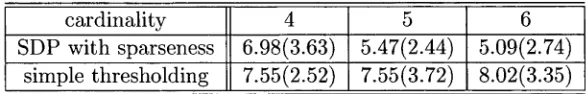
The second experiment is conducted on the Wine data described in Table 2.1. St, and Sv are constructed using SDP] using the same parameters shown in Table 2.1. The final projected dimension is 8. We want each column of W to be sparse. In other words, only a subset of features are selected. We compare our performance against the simple thresholding method [7]. Table 2.6 reports the classification

(2.9) is written into 1T(Z+ + Z_) 1 < (~)\/d and Z+ > 0. Z_ > 0 (element-wise non-negative). Here 1 is a column vector with all elements being ones.

error. As expected, the proposed algorithm performs better than the simple thresholding method.

cardinality 1 5 6

SDP with sparseness 6.98(3.63) 5.47(2.44) 5.09(2.74) simple thresholding 7.55(2.52) 7.55(3.72) 8.02(3.35)

Table 2.G: Classification error of a 3-NN classifier on the Wine dataset w.r.t. the cardinality of each row of W. Each case is run 20 times.

2 .7

C o n c lu sio n

In this work we have presented a new supervised dimensionality reduction algorithm. It has two key components: a global optimization strategy for solving the trace quotient problem; and a new trace quotient cost function specifically designed for linear dimensionality reduction. The proposed algorithms are

consistently better than LDA. Experiments show that our algorithms’ performance is comparable to the LMNN algorithm but with computational advantages. Future work will be focused on the following directions. First, we have confined ourself to

[image:47.526.120.413.145.192.2]

[image:48.526.14.515.83.788.2]

Figure 2.2: Subfigures (1)(2) show the data, projected into 2D using PCA and LDA. Both fail to recover the data structure. Subfigures (3)(4) show the results obtained by the two SDPs proposed in this chapter. The local structure of the data is pre­ served after projected by SDPs. Subfigures (5)(6) are the results when the rear eight dimensions are extremely noisy. In this case the neighboring relationships based on the Euclidean distance in the input space are completely meaningless. Subfigures (7)(8) successfully recover d ata’s underlying structure given user-provided neighbor­ hood graphs.

(1) PCA

. ••

X ■ - e ____ _

’J-A.

■X ■v -V-‘ Vk

•- A ■ i :

*

:■ r;v

■

-(3) SDPi, k = 230, k' = 5 (4) SDP2. fc = 5,fc' = 5

(5) SDPi, k= 230, k' = 5

.V,/ :--dp- v,,.,.

- K

r p K .

-* t

&

0

X

■V

. 7 dr J •?

• ■ * .

(6) SDPa, k= 5.k' = 5

\ " "\V.

X ■ V

v 0 i i

A

*•

. J

Figure 2.3: Cardinality of W v.s. 0 . The error bar shows the standard deviation averaged on 40 runs.

0.6

0 .4

0 .2

- 0.2

- 0 . 4

- 0.6

I 2 3 4 5 6 7 8 9 10

[image:49.526.13.515.28.610.2]

C hapter 3

P S D B o o st: M a tr ix - G e n e r a tio n

L in e a r P ro g ra m m in g for

M a h a la n o b is M e tric L e a rn in g

In this chapter, we consider the problem of learning a positive semidefinite matrix. The critical issue is how to preserve positive semidefiniteness d u r in g the course of learning. Our algorithm is mainly inspired by LPBoost [13] and the general greedy convex optimization framework of Zhang [54]. We demonstrate the essence of the algorithm, termed PSDBoost (positive semidefinite Boosting), by focusing on a few different applications in machine learning. The proposed PSDBoost algorithm extends traditional Boosting algorithms in that its parameter is a positive

semidefinite matrix with trace being one instead of a classifier. PSDBoost is based on the observation th at any trace-one positive semidefinite matrix can be

3.1

In tr o d u c tio n

Column generation (CG) [33] is a technique widely used in linear programming (LP) for solving large-sized problems. Thus far it has mainly been applied to solve problems with linear constraints. The proposed work here which we dub matrix generation (MG) extends the column generation technique to noil-polyhedral semidefinite constraints. In particular, as an application we show how to use it for solving a semidefinite metric learning problem. The fundamental idea is to

rephrase a bounded semidefinite constraint into a polyhedral one with infinitely many variables. This construction opens possibilities for use of the highly developed linear programming technology. Given the limitations of current semidefinite programming (SDP) solvers to deal with large-scale problems, the work presented here is of importance for many real applications.

The choice of a metric has a direct effect on the performance of many algorithms such as the simplest k-NN classifier and some clustering algorithms. Much effort has been spent on learning a good metric for pattern recognition and data mining. Clearly a good metric is task-dependent: different applications should use different measures for (dis)similarity between objects. We show how a. Mahalanobis metric is learned from examples of proximity comparison among triples of training data. For example, assuming that we are given triples of images a,, a a n d (a,, a, have same labels and a,, a^ have different labels, a* G M/}), we want to learn a metric between pairs of images such that the distance from a j to a * ( d is t^ ) is smaller than from a^ to a,; (d ist^ ). Triplets like this are the input of our metric learning algorithm. By casting the problem as optimization of the inner product of the linear transformation matrix and its transpose, the formulation is based on solving a semidefinite program. The algorithm finds an optimal linear