White Rose Research Online URL for this paper:
http://eprints.whiterose.ac.uk/141130/
Version: Accepted Version
Article:
Gonzalez-Aviles, J.J., Guzman, F.S., Fedun, V. et al. (4 more authors) (2019) In situ
generation of coronal Alfvén waves by jets. Monthly Notices of the Royal Astronomical
Society. ISSN 0035-8711
https://doi.org/10.1093/mnras/stz087
This is a pre-copyedited, author-produced PDF of an article accepted for publication in
Monthly Notices of the Royal Astronomical Society following peer review. The version of
record J J González-Avilés, F S Guzmán, V Fedun, G Verth, R Sharma, S Shelyag, S
Regnier; In situ generation of coronal Alfvén waves by jets, Monthly Notices of the Royal
Astronomical Society is available online at: https://doi.org/10.1093/mnras/stz087
[email protected]
https://eprints.whiterose.ac.uk/
Reuse
Items deposited in White Rose Research Online are protected by copyright, with all rights reserved unless
indicated otherwise. They may be downloaded and/or printed for private study, or other acts as permitted by
national copyright laws. The publisher or other rights holders may allow further reproduction and re-use of
the full text version. This is indicated by the licence information on the White Rose Research Online record
for the item.
Takedown
If you consider content in White Rose Research Online to be in breach of UK law, please notify us by
4School of Mathematics and Statistics, The University of Sheffield, Hicks Building, Hounsfield Road, Sheffield S3 7RH, UK
5Space Research Group-Space Weather, Departmento de Física y Mathemáticas, Universidad de Alcalá, Calle el Escorial, 19-21, 28805 Alcalá de Henares, Spain 6School of Information Technology, Deakin University, Burwood VIC 3125, Melbourne, Australia
7Department of Mathematics, Physics and Electrical Engineering, Northumbria University, Ellison Place, Newcastle upon Tyne NE1 8ST, UK
Accepted XXX. Received YYY; in original form ZZZ
ABSTRACT
Within the framework of 3D resistive MHD, we simulate the formation of a plasma jet with the morphology, upward velocity up to 130 km/s and timescale formation between 60 and 90 s after beginning of simulation, similar to those expected for Type II spicules. Initial results of this simulation were published in Paper (e.g.,González-Avilés et al. 2018) and present paper is devoted to the analysis of transverse displacements and rotational type motion of the jet. Our results suggest that 3D magnetic reconnection may be responsible for the formation of the jet in Paper (González-Avilés et al. 2018). In this paper, by calculating times series of the velocity componentsvxandvyin different points near to the jet for various heights we find transverse oscillations in agreement with spicule observations. We also obtain a time-distance plot of the temperature in a cross-cut at the plane x=0.1 Mm and find significant transverse displacements of the jet. By analyzing temperature isosurfaces of 104K with the distribution of vx, we find that if the line-of-sight (LOS) is approximately perpendicular to the jet axis then there is both motion towards and away from the observer across the width of the jet. This red-blue shift pattern of the jet is caused by rotational motion, initially clockwise and anti-clockwise afterwards, which could be interpreted as torsional motion and may generate torsional Alfvén waves in the corona region. From a nearly vertical perspective of the jet the LOS velocity component shows a central blue-shift region surrounded by red-shifted plasma. Key words: magnetohydrodynamics (MHD) – methods: numerical – Sun: atmosphere
1 INTRODUCTION
In the solar atmosphere, jet-like structures, defined as an impul-sive evolution of collimated bright or dark structure are observed in a wide range of environments. In particular, the upper chromo-sphere is full with spicules, thin jets of chromospheric plasma that reach heights of 10,000 km or move above the photosphere.
Al-though spicules were described bySecchi (1878), understanding their physical nature has been a whole area of research (Beckers et al. 1968;Sterling 2000). There are two types of spicules, the first type of spicules are so-called Type I, which reach maximum heights of 4-8 Mm, maximum ascending velocities of 15-40 km s−1, have a lifetime of 3-6.5 minutes (Pereira et al. 2012), and show up and downward motions (Beckers et al. 1968;Suematsu et al. 1995). These Type I spicules are probably the counterpart of the
⋆
E-mail:[email protected] (JJGA)
dynamic fibrils. They follow a parabolic (ballistic) path in space and time. In general the dynamics of these spicules is produced by mangneto-acoustic shock waves passing or wave-driving through the chromosphere (Shibata et al. 1982;De Pontieu et al. 2004; Hansteen et al. 2006;Martínez-Sykora et al. 2009;Matsumoto & Shibata 2010;Scullion et al. 2011).The second type of spicules are called Type II, which reach maximum heights of 3-9 Mm (longer in coronal holes) and have lifetimes of 50-150 s, shorter than that of Type I spicules (De Pontieu et al. 2007a;Pereira et al. 2012). These Type II spicules show apparent upward motion with speeds of order 30-110 km s−1. At the end of their life they usually exhibit rapid fading in chromospheric lines (De Pontieu et al. 2007b). It has been suggested from observations that Type II spicules are con-tinuously accelerated while being heated to at least transition region temperatures (De Pontieu et al. 2009,2011). Other observations indicate that some Type II spicules also show an increase or a more complex velocity dependence with height (Sekse et al. 2012).
outflow. In the Ca II H line they are seen to sway transversely with amplitudes of order 10-20 km s−1 and periods of 100-500 s (De Pontieu et al. 2007b;Tomczyk et al. 2007;Zaqarashvili & Erdélyi 2009;McIntosh et al. 2011;Sharma et al. 2017), suggesting gen-eration of upward, downward and standing Alfvén waves (Okamoto & De Pontieu 2011;Tavabi et al. 2015), the generation of MHD kink mode waves or Alfvén waves due to magnetic reconnection (Nishizuka et al. 2008;He et al. 2009;McLaughlin et al. 2012; Kuridze et al. 2012) or due to magnetic tension and ambipolar difussionMartínez-Sykora et al. (2017). For instance,Suematsu et al. (2008) suggest that some spicules show multi-thread structure as result of possible rotation. Another possible motion of Type II spicules is the torsional one as suggested byBeckers (1972) and Kayshap et al. (2018), and established using high-resolution spec-troscopy at the limb (De Pontieu et al. 2012). According to the latter, Type II spicules show torsional motions rotational speeds of 25-30 km s−1. In addition, the continuation of this kind of motion in the transition region and coronal lines suggest that they may help driving the solar wind (McIntosh et al. 2011).
There are other types of motion less well established, for in-stanceCurdt & Tian (2011) andCurdt et al. (2012) suggest that the spinning motion of Type II spicules can explain the tilts of ultra-violet lines in the so-called explosive events producing larger-scale macro spicules. These spectral-line tilts were observed at the limb and also attributed to spicule rotation (Beckers 1972). At smaller scales, evidence of rotating motions has been deduced for the chro-mospheric/transition region jet events (Liu et al. 2009,2011). In addition,Tian et al. (2014) using the IRIS instrument found trans-verse motions as well as line broadening attributed to the existence of twist and torsional Alfvén waves. At the photospheric level, there is evidence that a fraction of spicules present twisting motions ( Ster-ling et al. 2010a,b;De Pontieu et al. 2012). Beyond the resolution of imaging instruments, the spectrum of explosive events can also be interpreted as arising from the fast rotation of magnetic struc-tures (Curdt & Tian 2011;Curdt et al. 2012). Apart from the small scale jets, Doppler images have shown that several coronal jet events present strong rotational motion, diagnosed with blue-red shift observed on opposite sides of each jet (Dere et al. 1989;Pike & Mason 1998;Cheung et al. 2015).
In this paper, we show that the jet with characteristics of a Type II spicule, obtained in the numerical simulations presented inGonzález-Avilés et al. (2018) shows transverse displacements and rotational type motion initially clockwise and anti-clockwise afterwards, that could be a driver to excite torsional Alfvén waves directly in the corona.
The summary of the model and numerical methods are de-scribed in Section2. Section3describes the analysis of the plasma motions in the jet. In Section4, we present our final comments and conclusions.
2 SUMMARY OF THE MODEL AND NUMERICAL METHODS
The details of the numerical methods can be found in González-Avilés et al. (2018) and a brief summary is the following. We solve the resistive 3D MHD equations including the constant gravity field at the Sun’s surface. We integrate the Extended Generalized Lagrange Multiplier (EGLM) resistive MHD (Jiang et al. 2012) using High Resolution Shock Capturing methods with an adaptive choice of Flux formula between HLLC and HLLE, combined with MINMOD and MC limiters.
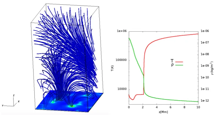
For the initial magnetic field, we use a 3D potential (current-free) configuration extrapolated from a simulated quiet-Sun pho-tospheric field, obtained from a large-scale, high-resolution, self-consistent simulation of solar magnetoconvection in a bipolar pho-tospheric region with the MURaM code (Vögler et al. 2005;Shelyag et al. 2012). The computational box has a size of 480×480×400 pixels, with a spatial resolution of 25 km in all directions.The
mag-netic field lines of the 3D configuration are shown in the left of Fig.1, and it is in this domain where the cross-cuts and further analysis are performed.
In order to model the atmosphere we choose the numerical domain to cover part of the interconnected solar photosphere, chro-mosphere and corona (see Fig.1). For this the atmosphere is initially assumed to be in hydrostatic equilibrium. The temperature field is considered to obey the semi-empirical C7 model of the chromo-sphere transition region (Avrett & Loeser 2008) and is distributed consistently with observed line intensities and profiles from the SUMER atlas of the extreme ultraviolet spectrum (Curdt et al. 1999). The photosphere is extended to the solar corona as described byFontela et al.(1990) andGriffiths et al.(1999). The temperature
T(z)and mass densityρ(z)are functions of heightzand are shown in Fig.1, where the transition region shows its characteristic steep gradient.
Once the magnetic field and atmosphere model are set in the computational domain (240×240×400 grid cells with a resolution of 25 km in each direction), the plasma evolves due to the inclusion of resistivity according to the EGLM equations. For our analysis, we focus on a 3D numerical box with unigrid discretization of size
x ∈[0,6],y∈[0,6],z ∈[0,10] Mm. In Section3, we analyze the
transverse and rotational motions in the jet and their observational signatures.
3 PLASMA MOTIONS IN THE JET
3.1 Transverse motions
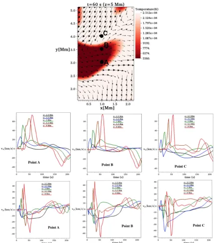
A property to look into is the transverse displacement of the jet investigate if it is actually oscillating in a kink-like manner. We measure the velocity componentsvxandvyin time at three different points near and within the spicule, points A (x=1,y=3,z) Mm, points B (x=1,y=3.5,z) Mm and points C (x=1,y=4,z) Mm, for various values ofz. Near these points the vector velocity field rotates as is illustrated at the top of Fig.2. We measure the value of the velocity components at heightsz=2.5, 3.5, 5, 6.5 and 8 Mm. The results displayed in Fig.2tell us about the motion along thexandy
directions. For example the horizontal component of velocityvxat the various heights in point A shows transverse displacements with high amplitudes at the top of jet and small at the bottom. We can also see a change of sign, which indicates a transverse oscillation of at least one period. The behavior ofvx at points B and C is similar to that at point A. In the case of thevycomponent at point A, we can see strong motions at the top, in particular there is a clear change of sing between 0 and 100 s, then we can identify oscillatory behavior at all heights, which is also clear at points B and C. By comparing the behavior ofvxandvywe can conclude that the jet shows rotational motion, i.e. velocity components are out of phase, which will be reinforced by the following analysis.
Figure 1.(Left) Magnetic field lines in the 3D domain at initial time. (Right) Temperature and mass density as a function of heightzfor the C7 equilibrium solar atmosphere model.
motion at a height of 7 Mm along a horizontal slice of length 3 Mm (blue line) centered at the mid-point of the domain in the y-direction (black line) as shown on the left of Fig.3. A time-distance plot of the logarithm of temperature along this slice as a function of time is shown on the right of Fig.3. From the time-distance plot we can see that from timet=50 s the jet starts moving to the left until about timet=150 s, jet starts moving to the right until it is displaced a horizontal distance of 3 Mm. This shows that simulated jet actually has a significant transverse motion during its lifetime. This phenomena is also observed widely in spicule observations, see e.g.,De Pontieu et al. (2007b). To estimate the average speed of the transverse displacements, we indicate the center of the jet at the the times of maximum and minimum displacement up to 150 s with horizontal dashed blue lines on the right of Fig.3. The distance between the two lines is about 0.7 Mm (700 km) and the time between them is about 100 s, therefore the average speed is about 7 km s−1.
3.2 Rotational motions
Another important property of Type II spicules to look at, is whether they are twisted, rotate or show an azimuthal flow component. Doppler shift observations of various emission lines in the limb suggest that Type II spicules are rotating (De Pontieu et al. 2012; Sekse et al. 2013;Sharma et al. 2017). From our simulation it is possible to study the behavior of the velocity componentsvxand
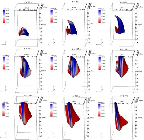
vz inside the jet in order to track possible rotational or twisting motions. A similar analysis was carried out byPariat et al. (2016) to identify torsional/twisting motions of coronal jets. In our case we show temperature contours with constant value of 104 K colored with the distribution ofvxat timest =30, 45, 60, 90, 105, 120, 150, 180 and 210 s in Fig.4.
For the perspective used in this case, the blue color represents motion toward the reader and red color represents motion away from the observer. For instance, at timet=30 s the jet starts to de-velop and shows both red and blue-shifted plasma. By timest=45 and 60 s, the motions are predominantly towards the observer with counter-motion developing at the top of the jet. At timet=90 s, the predominant motion towards the observer and some counter-motion still persists at the top of the jet. This dual behavior lasts through
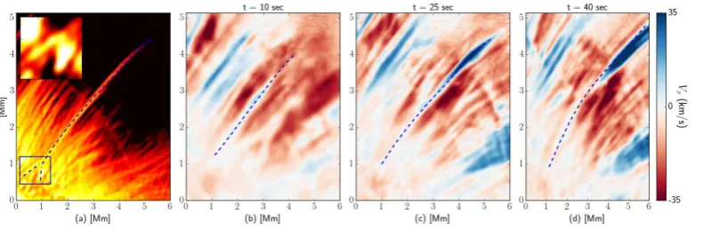
timest=105 andt=120 s. At timest=150, 180 and 210 s the jet shows a velocity structure represented by a red-blue asymmetry across its width. The time evolution of the jet from the simulation (Fig.4) also shows strong resemblance to the observations of a spicule seen off-limb in Hα(Fig.5).The imaging-spectroscopy
data used in the study was taken from the CRisp Imaging Spec-troPolarimeter (CRISP) at the Swedish Solar Telescope (SST) on 05 June 2014, during 11:53-12:34 UT, centered at xc=876′′,
yc = 343′′. The data was processed using the Multi-Object
Multi Frame Blind Deconvolution (MOMFBD;van Noort et al.
(2005)) image restoration technique. The off-limb region was scanned at±4 positions w.r.t. the line core (6563 Å) on the line
profile, with final science data had a pixel size of0′′.059 (∼43
km), angular resolution of0′′.13 (∼86 km) and a cadence of
5 sec. The dataset was also used previously byShetye et al.
(2016), to compare the image restoration techniques for chro-mospheric features.The unsharp mask intensity image (Fig.5(a)) of this spicule suggests it is launched from an inverted Y-shape structure (Shibata et al. 2007;He et al. 2009), associated with reconnection. The estimated Doppler shift profile (Vx), at discrete time-steps of the spicule evolution show striking similarities with the simulated jet. (Fig.5(b)) showcases the early rise-phase of the spicule (t = 10 s) as it starts to penetrate through the ambient chromospheric environment, as seen in Fig.4(t =30 s). At the middle-phase of it’s evolution (Fig.4,t=105 s), the spicule attains a mainly blue-shift Doppler profile, indicating bulk motion towards the observer as shown (Fig.5(c)). However, at the late-phase of the spicule’s ascent, the apex has developed an asymmetric red-blue Doppler profile (Fig.5(d)), indicating rotational motion, similar to the simulated jet (Fig.4, t = 180 s). The rotational motion is prevalent at height above 3 Mm, as is also seen in the simulation.
Also, the diagnostics shown in the time series of the velocity components at points A, B, and C in Fig.2together with Figs.4 indicate rotational motions of the jet.
Apart from the comparison of the red-blue shift with the observations, we can also link thexcomponent of the magnetic fieldBxfrom our simulation to the line of sight measurements
of the magnetic fields in spicules (López Ariste & Casini 2005;
Figure 2. In the top we show the region wherevxandvyare measured. The color labels the temperature in the planez=5 Mm at timet=60 s, where the
structure of spicule and the circulation of the vector velocity field is clearly seen. In the middle and bottom panels we show the time series ofvxandvyin km
s−1of the volume elements at the points A, B and C measured at various planes of constant height.
K colored with the distribution of Bx at different times. For
instance, at timet=30the jet shows mainly positive values of
the magnetic field, a behavior that lasts untilt=60s. At time
t=90s, we can see the appearance of negative values from the
bottom of the jet, which last untilt=120s. At the three last
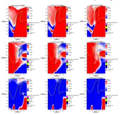
times t=150, 180 and 210 s the negative values appear from the top of the jet. In addition, in Fig.7we show the magnetic field componentsBx,By,Bz and temperature contours in a
cross-cut atx=0.1 Mm for three different times, this figure is similar
to the Figs. 5, 6 and 7 of paperGonzález-Avilés et al. (2018). For instance at the top of Fig.7, we can see positive values of Bx along the jet and the predominance of negative values at
the bottom of the jet for the three times. At the middle, we can see negative values ofBy at the top of the jet, while there is
a predominance of positive values ofByat the bottom for the
three times. At the bottom, we see that the Bz component is
predominantly negative along the jet for the three times.
3.3 Vertical motions
Figure 3.(Left) Snapshot of the logarithm of temperature (K) at timet=60 s, vertical line in black aty=3 Mm and horizontal line in blue fromy=1.5 Mm
toy=4.5 Mm atz=7 Mm. (Right) The time-distance plot of logarithm of temperature (K) and dashed lines to estimate the average transverse speed.
and 120 s, the amplitude of vertical motion start to decrease at the bottom of the jet. Finally, at timest =150, 180 and 210 s the jet starts moving downwards, in particular this behavior is consistent with the observed vertical motion with velocities of order 110 km s−1in Type II spiculesSkogsrud et al. (2014).
4 CONCLUSIONS
In this paper by analyzing temperature isosurfaces to localize the jet, together with the analysis of the horizontal velocity components, we find that the development of a red-blue asymmetry across the jet is due to rotational motion. Interestingly, the rotational motion is initially clockwise and then begins to move in an anti-clockwise direction, indicating the presence of torsional motion. By analyzing the time series ofvx and vy at points near and within the jet at different heights we showed that the rotational motion is generated in its upper region. In addition, by calculating a time-distance plot of the logarithm of temperature in a horizontal cross-cut at a height of 7 Mm it was shown that the jet also undergoes a considerable transverse displacement.
Additionally, we have presented observational support of ro-tational motion in an off-limb spicule appearing in the corona (and not being generated from below) in Fig.5(d). We can also see the simulated jet has a dual behavior (i) transverse motion at the foot (0-3 Mm) and (ii) twisted motion at the middle and top parts (3-10 Mm). The rotational type motion (initially clockwise and after anti clockwise) can be interpreted as torsional starting at the top of the jet, when it reaches a region where the magnetic field dominates
β < 1 as shown in Fig. 9and the Lorentz force is also bigger than pressure gradients|J×B| > |∇p|as shown in Fig. 7 of Pa-perGonzález-Avilés et al. (2018). This is important as it shows that torsional waves can be generated directly in the corona and therefore the whole wave energy (i.e without any loses due to prop-agation from the photosphere and dynamic chromosphere to the corona, as is usually suggested can be dissipated in the corona. For example, regions with (β <1) are perfect for the decay of torsional Alfvén waves into kinetic Alfvén waves, see e.g. cross-scale nonlin-ear coupling and plasma energization by Alfvén waves (Voitenko & Goossens 2005), excitation of kinetic Alfvén turbulence by MHD waves and energization of space plasmas (Voitenko & Goossens
2004) or the transformation of MHD Alfvén waves in space plasma (Fedun et al. 2004).
From a nearly vertical perspective of the jet, the vertical com-ponent of the velocity shows a blue-red shift, that is similar to the observed in the transition region and coronal lines as shown in Fig. 18 ofMartínez-Sykora et al. (2013), where the Doppler shifts correspond to velocities within the range -8 to 8 km s−1. Finally, although there is no magnetoconvection, in the simulated plasma jet we conclude that rotational motion can still occur naturally at coronal heights without the need of any photospheric driver, e.g., granular buffeting or vortex motion. In fact, we have shown that such jets could be an in-situ driver of torsional Alfvén waves in the corona.
ACKNOWLEDGMENTS
Figure 4. Snapshots of a temperature contour at various times. The jet is represented by an isosurface of the plasma temperature equal to 104K. The color
code labels the value ofvx. In this perspective blue indicates motion toward the reader and red toward inside the page.
REFERENCES
Avrett, E. H., & Loeser, R. 2008, ApJS, 175, 229 Beckers, J. M. 1968, Sol. Phys., 3, 367 Beckers, J. M. 1972, ARA&A, 10, 73
Centeno, R., Trujillo Bueno, J., & Asensio Ramos, A. 2010, ApJ, 708, 1579 Cheung, M. C. M., De Pontieu, B., Tarbell, T. D., et al. 2015, ApJ, 801, 83 Curdt W., Heinzel P., Schmidt W., Tarbell T., Uexkull V., Wilken V. 1999,
ed. A. Wilson (ESA SP-448;Noordwijk: ESA), 177 Curdt, W., & Tian, H. 2011, A&A, 532, L9
Curdt, W., Tian, H., & Kamio, S. 2012, Sol. Phys., 280, 417 De Pontieu, B., Erdélyi, R., & James, S. P. 2004, Nature, 430 536 De Pontieu, B., McIntosh, S., Hansteen, V. H. 2007a, PASJ, 59, 655 De Pontieu, B., McIntosh, S., Carlsson, M. et al. 2007b, Science, 318, 1574 De Pontieu, B., McIntosh, S. W., Hansteen, V. H., & Schrijver, C. J. 2009,
ApJ, 701, L1
De Pontieu, B., McIntosh, S. W., Carlsson, M., et al. 2011, Science, 331, 55
De Pontieu, B., Carlsson, M., Rouppe van der Voort, L. H. M., et al. 2012, ApJ, 752, L12
Dere, K. P., Bartoe, J.-D. F., & Brueckner, G. E. 1989, Sol. Phys., 123, 41 Fedun, V. N., Yukhimuk, A. K., & Voitsekhovskaya, A. D. 2004, Journal of
Plasma Physics, 70, 06
Fontela, J. M., Avrett, E. H., & Loeser, R. 1990, ApJ, 355, 700
González-Avilés, J. J., Guzmán, F. S., Fedun, V., Verth, G., Shelyag, S., & Regnier, S. 2018, ApJ, 856, 176
Griffiths, N. W., Fisher, G. H., Woods, D. T., & Siegmund, H. W. 1999, ApJ, 512, 992
Hansteen V. H., De Pontieu B., Ruoppe van der Voort L., van Noort M., Carlsson M. 2006, ApJ, 647, L73
He, J., Marsch, E., Tu, C., & Tian, H. 2009, ApJ, 705, L217
Jiang R. L., Fang C., Chen P. F. 2012, Comp. Phys. Comm., 183, 1617 Kayshap, P., Murawski, K., Srivastava, A. K., & Dwivedi, B. N. 2018,
arXiv:1805.02517
Figure 5.Left to right: Panels show a spicule (traced as dashed-line) off-limb, observed in Hαwavelength (a), with temporal evolution of the line-of-sight (LOS) Doppler velocity estimates (b-d). The unsharp-masked intensity image (a) show inverted Y-shaped structure (zoomed in inset) at the spicule footpoint (highlighted in box) suggestive of a magnetic reconnection process. Doppler estimates reveal the longitudinal rise of the spicule with its dominant motion towards the observer (b-c). The development of rotational motion is indicated by the enhanced red-blue asymmetric profile at the apex of spicule (d).
Jess, D. B., & Keenan, F. P. 2012, ApJ, 750, 51
Liu, W., Berger, T. E., Title, A. M., & Tarbell, T. D. 2009, ApJ, 707, L37 Liu, W., Berger, T. E., Title, A. M., Tarbell, T. D., & Low, B. C. 2011, ApJ,
728, 103
López Ariste, A., & Casini, R. 2005, A&A, 436, 325
McIntosh, S. W., De Pontieu, B., Carlsson, M., et al. 2011, Nature, 475, 477 McLaughlin, J. A., Verth, G., Fedun, V., & Erdélyi, R. 2012, ApJ, 749, 30 Martínez-Sykora, J., Hansteen, V., & Carlsson, M. 2009, ApJ, 702, 129 Martínez-Sykora, J., De Pontieu, B., Leenaarts, J., et al. 2013, ApJ, 771, 66 Martínez-Sykora, J., De Pontieu, B., Hansteen, V. H., Roupe van der Voort,
L., Carlsson, M., & Pereira, T. M. D. 2017, Science, 356, 1269 Matsumoto, T., & Shibata, K. 2010, ApJ, 710, 1857
Nishizuka, N., et al. 2008, ApJ, 683, L83
Okamoto, T. J., & De Pontieu, B. 2011, ApJ, 736, L24
Orozco Suárez, D., Asensio Ramos, A., & Trujillo Bueno, J. 2015, ApJ, 803, L18
Pariat, E., Dalmasse, K., DeVore, C. R., Antiochos, S. K., & Karpen, J. T. 2016, A&A, 596, A36
Pereira, T. M. D., De Pontieu, B., & Carlsson, M. 2012, ApJ, 759, 18 Pike, C. D., & Mason, H. E. 1998, Sol. Phys., 182, 333
Scullion, E., Erdélyi, R., Fedun, V., & Doyle, J. G. 2011, ApJ, 743, 14 Skogsrud, H., Roupe van Der Voort, L., & De Pontieu, B. 2014, ApJ, 795,
L23
Secchi, A., Die Sterne: Grundzuge der Astronomie der Fixsterne (Brock-haus, 1878)
Sekse, D. H., Rouppe van der Voort, L., & De Pontieu, B. 2012, ApJ, 752, 108
Sekse, D. H., Rouppe van der Voort, L., De Pontieu, B., & Scullion, E. 2013, ApJ, 769, 44
Sharma, R., Verth, G., & Erdélyi, R. 2017, ApJ, 840, 96
Shibata, K., Nishikawa, T., Kitai, R., & Suematsu, Y. 1982, Sol. Phys., 77,121
Shibata, K., Nakamura, T., & Matsumoto, T., et al. 2007, Science, 318, 5856 Shelyag, S., Mathioudakis, M., & Keenan, F. P. 2012, ApJ, 753, L22 Shetye, J., Doyle, J. G., & Scullion, E., et al. 2016, A&A, 589, A3 Sterling, A. C. 2000, Sol. Phys., 196, 79
Sterling, A. C., Harra, L. K., & Moore, R. 2010a, ApJ, 722, 1644 Sterling, A. C., Moore, R., & DeForest, C. E. 2010b, ApJ, 714, L1 Suematsu, Y., Wangm H., & Zirin, H. 1995,ApJ, 450, 411
Suematsu, Y., Ichimito, K., Katsukawa, Y., et al. 2008, in ASP Conf. Ser. 397, First Results From Hinode, ed. S. A. Matthews, J. M. Davis, & L. K. Harra (San Francisco, CA: ASP), 27
Tavabi, E., Koutchmy, S., & Golub, L. 2015, SoPh, 290, 2871
Tian, H., DeLuca, E., Cranmer, S. R., et al. 2014, Science, 346, 1255711 Tomczyk, S., McIntosh, S. W., Keil, S. L., Judge, P. G., Schad, T., Seeley,
D. H., & Edmondson, J. 2007, Science, 317, 1192
Van Noort, M., Der Voort, L. R. V. & Löfdahl, M. G. 2005, Sol. Phys., 228, 191