Effect of Solution Heat Treatment on Microstructure and Wear and Corrosion Behavior of a Two Phase β-Metastable Titanium Alloy

Int. J. Electrochem. Sci., 11 (2016) 3206 - 3226

International Journal of

ELECTROCHEMICAL

SCIENCE

www.electrochemsci.org

Effect of Solution Heat Treatment on Microstructure and Wear

and Corrosion Behavior of a Two Phase β-Metastable Titanium

Alloy

Khaled M. Ibrahim1,2, M. Mahmoud Moustafa1,3, Mubarak W. Al-Grafi1, Nader El-Bagoury2,4, Mohammed A. Amin4, 5,*

1

Taibah University, College of Engineering, P.O. Box. 344 Al-Madinah Al-Mounwara, Saudi Arabia

2

CMRDI, P.O. Box 87 Helwan, Cairo, Egypt

3

Production Engineering and Design Department, Minia University, Faculty of Engineering, Minia, Egypt

4

TAIF University, Chemistry Department, Faculty of Science, P.O. Box 888, El-Haweyah, Saudia Arabia

5

Department of Chemistry, Faculty of Science, Ain Shams University, 11566 Abbassia, Cairo, Egypt

*

E-mail: [email protected]

Received: 19 September 2015 / Accepted: 29 January 2016 / Published: 1 March 2016

A low cost beta titanium (LCB Ti) alloy with a composition of Ti-6.62Mo-4.53Fe-1.45Al-0.14O was subjected to solution heat treatment process at two different temperatures, namely 650 oC and 750 oC. Each heat treated process was followed by ageing at 500 °C for 4 hrs. The obtained microstructures were studied and their influence on the mechanical and chemical properties of the LCB Ti-alloy was reported. The Ti alloy that is heat treated at 650 °C (designated here as alloy I), showed a fine microstructure with 15% volume fraction of fine continuous α-phase at the β-grains. The microstructure of the Ti alloy when heat treated at 750 °C (alloy II) was coarse with 10% of discontinuous α-phase formed at the β-grains. A high tensile strength of 1492 MPa was obtained for alloy I due to its fineness microstructure. However, alloy II recorded a low strength of 1295 MPa due to its coarse α-β microstructure. The uniform corrosion characteristics of alloys I and II was studied in 3.5% NaCl solutions employing Tafel polarization, linear polarization resistance (LPR), and electrochemical impedance spectroscopy (EIS) techniques. The anodic behavior of these materials was also assessed adopting potentiodynamic anodic polarization and chronoamperometry measurements. The corrosion behavior of a spring steel alloy was also included for comparison. Alloy II recorded the highest (superior) corrosion resistance among the tested alloys. Microstructure features and spontaneous passivation of alloys I and II were used to account for their high corrosion resistance, as compared with spring steel.

1. INTRODUCTION

The non-aerospace use of titanium alloys such as suspension springs for automobiles and medical implants has become increasingly popular over the last 20 years due to their light weight, high ductility and high strength in conjunction with excellent corrosion resistance and outstanding biocompatibility [1-3]. Titanium alloys are normally classified by their structure into the groups of alpha, near-alpha, alpha-beta, metastable beta and beta alloys. Titanium alloys can also be classified based on the value of Al and Mo equivalent parameters. Al-equivalent value indicates the capacity of the alloy to obtain a given hardness, whereas the Mo-equivalent value indicates the capacity to obtain ultimate tensile strength and hardness in the aged condition [4-6].

In automotive industry, low cost beta (LCB) titanium alloy has been used in manufacturing suspension springs due to its low weight and high corrosion resistance [7, 8]. The main chemical composition of the LCB titanium alloy is (Ti-6.8Mo-4.5Fe-1.5Al). The low cost of LCB Ti-alloy compared to other Ti alloys is due to using an inexpensive Fe-Mo master alloy which is widely used in steel industry [9, 10]. This composition contains some elements forming beta phase such as Mo and Fe and also other forming alpha phase as Al. The advantages of existing β phase in Ti-alloys are excellent workability, good hardening ability, corrosion resistance and excellent fatigue/crack propagation behavior. On the other hand, the presence of the alpha phase in the microstructure of the LCB Ti-alloys can be characterized generally by high creep resistance that is superior to these alloys, and is preferred for high-temperature applications. LCB Ti-alloy with the composition of Ti-6.8Mo-4.5Fe-1.5Al is designed to achieve beta phase stability at room temperature with the least amount of expensive alloying elements, thus conferring a cost advantage compared with other beta alloys [11-13]. By applying solution treatment and ageing, some α-phase will precipitate at the grain boundaries and fine secondary α-phase will precipitate inside the grains [14-16].

The mechanical properties of titanium alloys are influenced by individual properties of α and β phases, their arrangement and volume fraction. For example, the α-phase has lower density than the β-phase due to the fact that the predominant element Al in α-β-phase has lower density than the predominant elements of Mo or V in β-phase. The density value of β-titanium alloys is about 4.5 g/cm3

[17].LCB Ti-alloy has been found to have a good mechanical properties, such as high strength (UTS≈1350 MPa), yield strength (YS≈900 MPa) and good ductility (total elongation ≈ 18%) [18, 19].

with SEM examinations. Potentiodynamic anodic polarization and chronoamperometry measurements were used to assess the anodic behavior of such alloys.

2. EXPERIMENTAL WORK

The LCB material employed here was prepared by melting in a vacuum induction furnace as bars with 30 mm diameter and 300 mm long. Then the cast bars hot forged at a temperature of 760 °C, in the range of α+β zone, to reduce the diameter into 10 mm. The nominal composition of the investigated LCB titanium alloy is Ti-1.45Al-6.62Mo-4.53Fe-0.14O. The samples were solution treated below the beta transus at two different temperature, namely 750 °C and 650 °C for 30 min. (in the α-β phase field) and then quenched in water in order to retain the β-phase at room temperature in a metastable state. After solution treatment, ageing treatment was conducted at a constant temperature of 500 °C for 4 hrs. The microstructure of heat-treated specimens were prepared using the standard metallographic techniques, and etched using Kroll’s reagent containing 10 mL HF, 5 mL HNO3 and 85

mL water. The specimens were then examined with a scanning electron microscopy (SEM).

In order to observe the influence of using two different solution temperatures, mechanical and chemical tests were performed on the samples. Vickers hardness tester with a load of 10 Kg was used to evaluate the hardness of the investigated samples. Tensile test was performed on threaded cylindrical specimens having a gage length and diameter of 20 mm and 4 mm, respectively. The tensile test was performed at room temperature and also at a high temperature of 600 °C. Pin-on-ring test rig was used to evaluate the wear behavior of the investigated LCB titanium alloy at room temperature. The test sample dimension was 8-mm in diameter and 12-mm long in which it was pressed against a rotated ring made of hard stainless steel with a surface hardness of 63 HRC and 0.2 μm surface roughness. Prior to the wear test, the surface of the rotated ring was ground with a 1000-grit emery paper. The sliding speed was 1 m/s which was equivalent to 265 rpm, and the sliding time was 30 min. The applied load was selected to be 100, 200, 300, 400, and 500 g. The surface morphology of some selected samples was investigated by stereo and optical microscopes to determine the wear mechanism in each case. Before wear test the weight of specimen was taken accurately using an electronic balance with an accuracy of 0.001 g. After the test, the sample was taken out carefully so that the debris’s were removed from the valleys of the specimen and exact wear materials can be measured. Once again weight was taken carefully using the above balance and the difference in weight was calculated. All the above tests and measurements were carried out at least three times under identical conditions to make sure the reliability of the data, which was found to be so good, and the mean values were calculated and reported.

For electrochemical measurements, sheets of dimensions (0.7 cm) x (1.5 cm) x (0.25 cm; thickness) were cut from the coupons of the employed alloys. Prior to electrochemical measurements, all sides of the sheets were isolated to offer an active flat rectangular shaped surface of (0.7 x 0.25 = 0.175 cm2), immersed into the test solution. Open-circuit potential (EOC) of the tested samples is

standard cell system of capacity 100 mL. This cell contains three compartments for working, platinum spiral counter and reference electrodes. A Luggin–Haber capillary was also included in the design. The reference electrode was a saturated calomel electrode (SCE), and used directly in contact with the working solution. The measurements were carried out in naturally aerated solutions at 25 oC (±1 ◦C). The temperature is maintained constant at the room temperature using a water thermostat.

Linear polarization resistance (LPR), Tafel plots, ac impedance measurements are the electrochemical techniques employed in the present work to assess the uniform corrosion characteristics of the tested alloys. The LPR curves were recorded in the potential range of -20 to +20 mV with respect to EOC at a scan rate of 0.2 mV s-1. The potentiodynamic polarization curves were

recorded in a potential window of -0.25 to 0.25 V vs. Ecorr at a scan rate of 1.0 mV s-1. Electrochemical

impedance measurements were carried out at Ecorr in the frequency range 100 kHz–10 mHz with an

amplitude of 5 mV. Before each run, the open circuit potential of the working electrode was measured as a function of time during 3 h to attain steady state. The order of performing electrochemical measurements was: (i) Chronopotentiometry (zero current); EOC vs. time (up to 3 h), followed by (ii)

LPR technique (Ecorr ± 20 mV; Ecorr ~ steady-state potential in the EOC vs. time plots), followed by (iii)

impedance measurements at Ecorr, and finally (iv) Tafel polarization (Ecorr ± 250 mV). As the later (i.e.,

Tafel polarization) is a destructive technique, the cell is cleaned, the test solution is replaced by a fresh one, and a cleaned set of electrodes was used for studying the anodic behavior of the tested alloys based on potentiodynamic anodic polarization and chronoamperometry techniques.

The potentiodynamic anodic polarization curves were recorded by changing the electrode potential automatically towards the anodic direction starting from -2.0 V(SCE) up to +2 V(SCE) at a potential scan rate of 1.0 mV s-1. The polarization plots were recorded as log current density (log j) against potential (E), after an open circuit stabilization of 3 h. Chronoamperometric measurements were carried out using a two step procedure, namely: the working electrode was first held at the starting potential for 60s to attain a reproducible electroreduced electrode surface. Then the electrode was held at constant anodic potential (Ea), where the anodic current was recorded as a function of time.

At least three separate experiments were carried out for each run to ensure reproducibility of results. The reproducibility of all employed electrochemical measurements was good. This good reproducibility was expected since a protracted immersion period (3 h) was undertaken to achieve a steady corrosion potential. However, it is important to point out that the various parameters obtained from these measurements are the mean values from the three independent experiments performed. The mean value and standard deviation of the results were calculated and reported.

The morphologies of the corroded surfaces of the tested alloys were examined by an Analytical Scanning Electron Microscope JEOL JSM 6390 LA. The compositions of such surfaces were determined using ZAF software to quantify the energy-dispersive X-ray spectroscopy (EDS) spectra obtained by an EDS attachment (JEOL EDS EX-54175JMU) on the JEOL SEM.

3. RESULTS AND DISCUSSION

for LCβ Ti alloy subjected to a solution heat treatment process at 650 oC and 750 oC, respectively. In each case, the solution heat treatment process is followed by ageing at 500 °C for 4 hrs.

3.1. Microstructure and mechanical properties

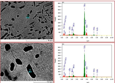
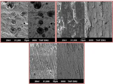
Figure 1. Microstructures of alloys I (images a) and II (images b).

Solution treatment process, which applied at temperature range below the β transus, as in the present study, maintains a microstructure with fine grains [4, 9, 19]. Consequently, this fine α-β structure provides a desirable combination of strength and ductility as well as wear property. The microstructures of alloys I and II are shown in Fig. 1. The microstructure of alloy I showed fine equiaxed β-grain structure with almost needle-like morphology of 15% primary α-phase, as shown in Fig. 1(images a1 and a2). Alloy II showed the same feature of microstructure, but with lower amount (~

10%) of the needle-like primary α-phase, Fig. 1 (images b1 and b2). The primary α-phase lies at the

process at 500 °C. Azimzadeh and Clement [3,20] reported that very fine ω-particles can precipitate after ageing in a temperature range of 390 °C to 460 °C. These ω-particles are acting as a nucleation site for the α-phase. We did not observe the ω-particles here, as the ageing process was applied at 500 °C. Therefore, the precipitation of α-phase has occurred in the absence of ω via heterogeneous nucleation mechanism [2]. In such case, the grain boundary α nucleation becomes increasingly important, as it can effectively control the precipitation process [20].

The α-phase of alloys I and II was analyzed using EDX to demonstrate the influence of the temperature of the solution heat treatment process on the element contents existing in that phase, inspect Fig. 2 and Table 1. Such analysis revealed that the Al content (mass, %) in the α phase of alloy I is higher than its content in alloy II. This can be explained on the basis that the higher solution temperature of 750 °C dissolved more Al-content as compared to the lower solution temperature of 650 °C. This amount of dissolved Al precipitates in the phase. This is because Al is considered as α-stabilizer element [21]. Meanwhile, Fe and Mo amounts in α phase decreased at 750 o

C compared to the samples solution treated at 650 oC, because these elements (Fe and Mo) are considered β-stabilizer elements [22]. By increasing the solution temperature, more Fe and Mo are precipitated in the β-phase rather than the α-phase. This in turn decreased the mass amount of Fe and Mo in the α-phase, and subsequently their content in the β-phase (the matrix) is increased. Hence the β-to-α transformation could be considered as a displacive transformation. Subsequently, a change in the chemical composition of the α and β phases takes place as a result of increasing the temperature of the solution heat treatment process from 650 oC to 750 oC. This change in chemical composition has occurred via migration of interstitial and substitutional atoms as in classical diffusion transformation [3].

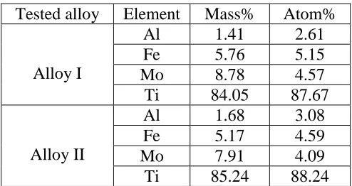
Table 1. Amounts of Al, Fe, Mo, and Ti in the α-phase existing in the matrix of alloys I and II.

Tested alloy Element Mass% Atom%

Alloy I

Al 1.41 2.61

Fe 5.76 5.15

Mo 8.78 4.57

Ti 84.05 87.67

Alloy II

Al 1.68 3.08

Fe 5.17 4.59

Mo 7.91 4.09

Ti 85.24 88.24

It is worth well known that the microstructure state of α-β strongly influences the mechanical properties of the investigated samples. The mechanical properties of the studied LCB alloy can be directly related to the state of α-precipitates in the microstructure. The amount of α-precipitates existing in the microstructure coincides well with the hardness values in both solution treatments, namely 650 oC and 750 oC. Alloy I recorded a hardness value of 455 HV, which is higher than that measured for alloy II (412 HV). This increased hardness of alloy I can be related to its high amount of α-precipitates as compared to the alloy II. The influence of solution temperature on tensile strength of alloys I and II was also studied at room temperature (RT) as well as at a high temperature of 600 °C. The obtained results showed that, for testing at RT, the tensile strength of alloy I (1492 MPa) is considerably higher than that of alloy II, 1295 MPa. This remarkable difference (197 MPa) in the tensile strength is attributed to the higher volume fraction (Vf) of the primary α-phase, secondary fine

α-precipitates in the β-matrix as well as the fineness of the microstructure of alloy I. The same behavior was also noticed for the samples tested at 600 °C, where alloy I recorded a tensile strength of 465 MPa and alloy II measured 387 MPa. For all tensile testing samples, the yield strength was slightly lower than the tensile strength [10]. This could be backed to the highly dislocation density inside the structure of the samples that resulted from the mechanical deformation during their fabrication processes. In addition, the presence of secondary fine α-precipitates in the β-matrix will also approximate the yield strength to the tensile strength. These factors will decrease the plasticity inside the materials. These are the reasons why the values of the yield strength of alloys I and II are slightly lower than those of the tensile strength.

0 100 200 300 400 500 600

1.6 2.0 2.4 2.8 3.2 3.6 4.0

Alloy I

Alloy II

Weigh

t l

oss x 10

2 /

g

cm

-2

Applied load / g cm-2

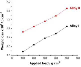
Figure 3. Weight loss vs. applied load of alloys I and II.

On the other hand, hardness and microstructure constituents play an important role in determining the weight loss of the studied samples. For alloy I, the microstructure contains high Vf of

the α-phase as well as fine secondary α-phase compared to alloy II [24]. It is also reported that the wear resistance of materials is determined by both strength or hardness and ductility, as described by the empirical equation of Archard, Eq. (1):

W = K (P/H) (1)

where W is the wear rate, P is the applied load, H is the hardness of materials, and K is a pre-factor related to the ductility of materials [25]. According to Eq. (1), the weight loss of alloy I is lower than that of alloy II, confirming the results of Fig. 4, because of the high hardness and strength of the former as compared to the later.

100 g 200 g 300 g

400 g 500 g

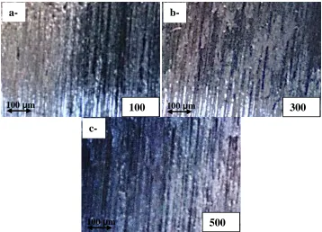
Figure 4. Optical macrographs of the wear scars at different applied loads for alloy I.

Figure 5. Worn surfaces at different applied loads for alloy I.

As shown in Fig. 5-a, the worn surface of the samples tested at low load of 100 g shows only scratches. These scratches become deeper with increasing the applied load up to 300 g. Also, delamination of wear debris started to appear over the worn surface, Fig. 5-b. By increasing the applied load further (500 g), the worn surface was covered with wear debris and the scratches became deeper, Fig. 5-c.

300 g

100 μm

b-

100 g

100 μm

a-

500 g

100 μm

3.2. Electrochemical studies

It is also proposed in this work to study the corrosion behavior of alloys I and II in 3.5% NaCl solutions. As a reference point, the corrosion behavior of spring steel is also included. The spring steel has been selected as a reference because both alloys (LCB Ti and spring steel) are used in manufacturing suspension springs for automotive industry.

3.2.1. Uniform corrosion studies

3.2.1.1. Monitoring open-circuit potential

The open-circuit potential (OCP) of alloys I and II was monitored during 3h of immersion in aerated non-stirred 3.5% NaCl solution at 25 °C, Fig. 6. The objective is to achieve a stable value and define domains of corrosion [26]. It is seen for the steel electrode (curve 1) that the potential changed quickly towards more negative values, as shown in the inset of Fig. 6. This indicates the initial dissolution process of the pre-immersion, air formed oxide film and the attack on the bare metal [27]. A steady potential was readily attained, corresponding to the free corrosion potential (Ecorr) of the

metal, as evidenced from polarization studies (see later). The open-circuit corrosion behavior of alloys I and II (curves 2 and 3) is completely different from that of the spring steel alloy (curve 1). There is a general tendency for alloys I and II to passivate, and the extent of their passivation depends upon the temperature of the solution heat treatment process. For alloy I, which is heat treated at 650 oC, the rest potential is first shifted to the less negative values reaching a maximum at a certain time then declined to a reasonably steady value, as clearly seen in the inset of Fig. 6.

0 1000 2000 3000 4000 5000 6000 7000 -0.60 -0.55 -0.50 -0.45 -0.40 -0.35 -0.30 -0.25 -0.20 -0.15 3 2

1 0 1000 2000 3000 4000 5000 6000 7000 -0.615 -0.610 -0.605 -0.600 -0.595 -0.590 -0.585 O C P / V vs S C E

Time / s

1000 2000 3000 4000 5000 6000 7000

-0.42 -0.40 -0.38 -0.36 O C P / V vs S C E

Time / s

O C P / V vs S C E

Time / s

Figure 6. Open-circuit potential (OCP) vs time measurements recorded for the three tested alloys in 3.5% NaCl solution at 25 °C. (1) Spring steel; (2) alloy I; (3) alloy II.

The high corrosion resistance of alloy II, as compared with alloy I, can be interpreted on the basis that elevating the temperature of the solution treatment process from 650 (alloy I) to 750 C (alloy II) decreases the volume fraction (Vf) of the  phase, that precipitated in the  matrix, revisit

Fig. 1. This in turn decreases the rate of corrosion due to the local galvanic cell between  and  phases in case of alloy II than in alloy I. Therefore, it can be concluded that the corrosion rate of alloy II (750 C) is lower than that of alloy I (650 C) due to the lower Vf of the α phase in the former alloy

than in the latter one.

3.2.1.2. Polarization studies

The uniform corrosion responses of the studied alloys were also established on the basis of Tafel polarization measurements that performed in aerated non-stirred 3.5% NaCl solutions at a scan rate of 1.0 mV s-1 at 25 oC. The obtained cathodic and anodic polarization curves are depicted in Fig. 8.

-1.4 -1.2 -1.0 -0.8 -0.6 -0.4

-8 -7 -6 -5 -4 -3 -2 -1 0

3

2

1

log (j / A cm

)

E / V(SC

E)

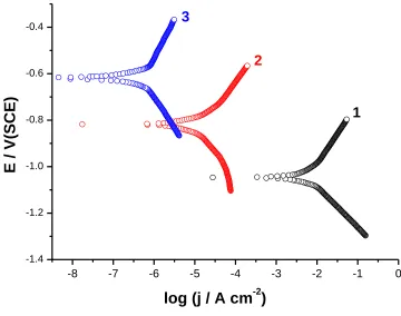
Figure 8. Cathodic and anodic polarization plots recorded for (1) spring steel, (2) alloy I, and (3) alloy II. Measurements were conducted in non-stirred naturally aerated 3.5% NaCl solutions at a scan rate of 1.0 mV s-1 at 25 oC.

mV), Fig. 8, and in the vicinity of the corrosion potential (E = Ecorr ± 20 mV), namely linear

polarization resistance (LPR) measurements, Fig. 9.

Table 2. Mean value (standard deviation) of the electrochemical kinetic parameters, derived from Tafel polarization and LPR measurements, recorded for spring steel and alloys I and II. Measurements were conducted in non-stirred naturally aerated 3.5% NaCl solutions at a scan rate of 1.0 mV s-1 at 25 oC.

Tested alloy Tafel polarization LPR method

-Ecorr /

mV(SCE)

-βc /

mV dec-1

βa /

mV dec-1

jcorr /

mA cm-2

Rp /

Ω cm2 jcorr /

mA cm-2 Alloy I 822(9.4) 380(3.6) 180(1.9) 2(0.03) x 10-2 2411() 2.2(0.04) x 10-2 Alloy II 622(6.8) 290(2.8) 330(3.2) 5.9(0.1) x 10-4 121861() 5.5(0.07) x 10-2 Spring steel 1050(11.6) 180(2.2) 270(2.9) 6.61(0.14) 7.41() 6.33(0.12)

Figure 8 reveals that the profile of the Tafel plots, particularly in the location of Ecorr and in the

magnitudes of the overpotentials of both the anodic and cathodic processes, change according to the type of the tested alloy. While the spring steel alloy exhibited the lowest anodic and catholic overpotentials (and hence higher rates of corrosion), alloy II recorded the highest overpotentials for both the anodic and cathodic processes. Moderate values are measured for alloy I. This is quite clear from the data of Table 2. Spring steel alloy recorded a jcorr value of 6.61 mA cm-2, which is 330 times

greater than that recorded for alloy I (2 x 10-2 mA cm-2) and more than 11,000 times greater than that measured for alloy II (5.9 x 10-4 mA cm-2), demonstrating the high corrosion resistance of alloy II.

-20 -10 0 10 20

-0.006 -0.004 -0.002 0.000 0.002 0.004

-20 -10 0 10 20 -6.0x10-6 -4.0x10-6

-2.0x10-6 _0.0

2.0x10-6

4.0x10-6

6.0x10-6

3 2

j / A cm-2

( E -Eco rr ) / m V 3 2 1

j / A cm-2

( E -E c or r

) / m

V

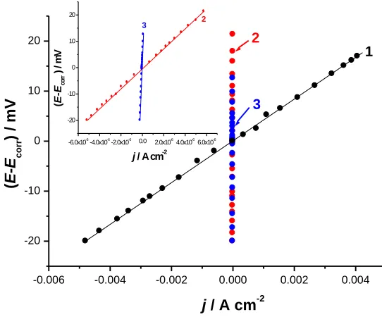
Referring to LPR measurements, Fig. 9, slopes from such linear plots show the polarization resistance Rp, defined as the tangent of a polarization curve at Ecorr [28].

Rp = (dE/dj)E=Ecorr (2)

Table 2 also presents the values of Rp for the three tested alloys. Values of the anodic and

catholic Tafel slopes, βa and βc, obtained from the analysis of the Tafel plots (Fig. 8 and Table 2),

together with the values of Rp obtained from LPR method (Fig. 9 and Table 2) are introduced in

Stern-Geary equation [29] to get accurate values for jcorr.

jcorr = B/Rp = {βa βc /2.303(βa + βc)} / Rp (3)

Results are also presented in Table 2. Obviously, a good agreement exists between the values of jcorr evaluated from the Tafel extrapolation method and those calculated from the LPR method. Here

again, alloys I and II recorded Rp values that are much higher than that measured for the spring steel

alloy. Generally, the increase in the Rp value suggests that the corrosion rate is decreased,

corresponding to improved corrosion resistance. As clearly seen in Table 2, alloy II recorded Rp value

of (121861 Ω cm2), which is 50 time greater than that of alloy I (2411 Ω cm2) and more than 1600 times greater than that measured for the spring steel alloy (7.41 Ω cm2

). These findings support the highest (superior) corrosion resistance of alloy II.

Further inspection of Table 1 reveals that the Tafel slopes, particularly the values of βc,

measured for alloys I and II (380 and 290 mV dec-1) are greater than that of the spring steel electrode, 180 mV dec-1. Almost similar results were previously obtained by M. Metikoš-Huković et al. [30], and very recently by our research group [31] during Al corrosion inhibition studies in perchloric acid solutions. Such higher values of βc can be attributed to the spontaneous passivation of Ti and

subsequent formation of a stable, substantially inert oxide film [30,31]. This passive film limits the reducing ability of Ti [32] and hence retards the reduction process at the surface by affecting the energetics of the reaction at the double layer, by imposing a barrier to charge transfer through the film, or both. The barrier-film model was a consistent way of explaining the high Tafel slopes for the HER observed [33].

3.4. Electrochemical Impedance Spectroscopy Measurements

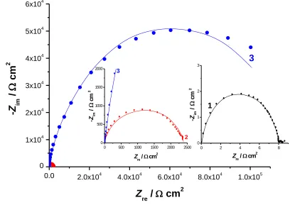
To gain more insight on the kinetics of the electrode processes and surface properties of the investigated alloys (alloys I and II), impedance measurements were carried out for each alloy at its Ecorr. The impedance response of spring steel was also included for comparison. The obtained

loop can be related to the combination of the charge-transfer resistance (Rct) of the corrosion process

and the corresponding capacitance (Cdl) at the electrode-electrolyte interface [34].

The depressed nature of these capacitive loops, caused by the generation of micro-roughness at the surface during the corrosion process [35,36], is confirmed from their mathematical analysis. Such analysis revealed that the center of the two capacitive loops lies below the real axis. In addition, the slopes of the log |Z| against log f plots (not included here) are not –1. To describe this response properly, a constant phase element, CPE, was used whose impedance, ZCPE, is given by the expression

[30,37]:

ZCPE = Q-1(jω)-n (4)

where Q is the CPE constant (a proportional factor), ω the angular frequency (in rad s-1

), j2 = -1 the imaginary number and n is the CPE exponent. The factor n is an adjustable parameter that usually lies between 0.50 and 1.0 [35].Values of n are usually related to the roughness of the electrode surface. The smaller value of n, the higher the surface roughness [35,36].

0.0 _2.0x104

4.0x104 6.0x104 8.0x104 1.0x105

0 1x104 2x104 3x104 4x104 5x104 6x104

0 500 1000 1500 2000 2500 0 500 1000 1500 2000 2 3 -Zim /  c m 2

Z_re /  cm2

1

0 2 4 6 8

0 1 2 3 -Zim /  c m 2

Z_re /  cm2

3

-Z

/



cm

Z

/

cm

Based on this, the CPE describes an ideal capacitor when n = 1. The value of Cdl can be

calculated for a parallel circuit consists of a CPE(Q) and a resistor (Rct), according to the following

formula [38]:

Q = (CRct)n / Rct (5)

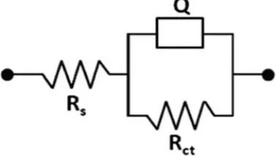
To determine the value of each impedance parameter described above, the measured impedance data were simulated using nonlinear-least square fitting analysis (NLS) software, based upon the electric equivalent circuit given in the inset of Fig. 11.

Figure 11. The equivalent circuit used to simulate the experimental impedance data.

A good fit with this model was obtained with our experimental data. It is observed that the fitted data match the experimental, with an average error of about 3–5%. The symbols in all impedance plots represent the experimental data, while the solid lines represent the best fits. The obtained fitting parameters are presented in Table 3.

Table 3. Mean value (standard deviation) of the electrochemical impedance parameters recorded for alloys I and II, in a comparison with spring steel. Measurements were conducted in non-stirred naturally aerated 3.5% NaCl solutions at the respective Ecorr at 25 oC.

Tested alloy

Rs /

Ω cm2 _{Ω cm}Rct / 2 Q /

Sn(ω-1 cm-2)

n Cdl /

µF cm-2

Alloy I 2.24(0.05) 2386(25.7) 8.13(0.09) 0.92 5.77(0.08) Alloy II 2.38(0.7) 121498(51) 1.97(0.04) 0.96 1.86(0.05) Spring steel 2.16(0.06) 7.99(0.12) 220.86(3.6) 0.81 49.92(0.7)

It follows that alloys I and II exhibit much higher impedance (Rct = 2386 Ω cm2 and 121498 Ω

cm2 for alloys I and II, respectively) than the spring steel alloy (Rct = 7.99 Ω cm2). The significantly

increased impedance (121498 Ω cm2

contrary, the smallest capacitance value (Q = 1.97 Sn(ω-1 cm-2) and C = 1.86 µF cm-2) was measured for alloy II, demonstrating its high corrosion resistance. Further inspection of Table 3 reveals that a good agreement between the values of Rp calculated from EIS measurements with those derived from

the LPR method (Table 2).

3.2.2. Anodic behavior

3.2.2.1. Potentiodynamic anodic polarization measurements

As previously shown, Tafel plots (Fig.8) provided us with general corrosion rate information of the three tested alloys with a relatively narrow potential range, 500 mV. The amount of information obtained from electrochemical corrosion measurements increased, as wider polarization potential ranges are used to generate the data. Potentiodynamic anodic polarization measurements are generated here with a wider potential range of 4000 mV, and provide additional information concerning corrosion kinetics and passivity of the tested alloys. Figure 12 shows the potentiodynamic anodic polarization curves recorded for the three tested alloys in 3.5% NaCl solutions at a scan rate of 1.0 mV s-1.

-2 -1 0 1 2

-8 -6 -4 -2 0

j pass

3 2 1

log (j / A cm

)

E /

V(SCE)

It can be seen that on positive going scan, the cathodic current density decreases gradually reaching its lowest value at Ecorr. The values of Ecorr obtained from Fig. 13 are almost close to those

obtained from the both the free corrosion behavior (EOC vs. time measurements, Fig. 6) and Tafel

polarization measurements, Fig. 8. The anodic excursion span of the spring steel electrode (curve 1) exhibits an active dissolution region near Ecorr due to the anodic dissolution of the spring steel. This

active dissolution region doesn’t exist in the polarization curves of alloys I and II, denoting high corrosion resistance due to spontaneous passivation.

Beyond Ecorr, a wide passive region forms, the current of which depends on the type of the

tested alloy. Passivity of alloys I and II (curves 2 and 3) originate from the formation of corrosion products and/or metal oxides layers on the alloy surface. Such layers possess some protective influence and reduce the active dissolution of the alloy (passivation). These results demonstrate that the oxide film is stable in this range of potential, and accordingly a very low current (designated here as the passive current, jpass) results. Passivity persists as the potential is increased till the end of the run, where

the rate of passive film formation equals that rate of its dissolution so that the oxide film hardly grows [39-43].

Further inspection of Fig. 12 demonstrates that the value of jpass, at any given potential within

the region of passivity, of alloy II is much lower than that for alloy I, confirming the high corrosion resistance of alloy II compared with alloy I. The situation is different for the spring steel alloy (curve 1), which exhibited extremely low corrosion resistance compared with alloys I and II, where the anodic current obviously enhances with the applied anodic potential. These findings reflect the weakness and thinning of the passive film promoted by the adsorption of Cl- anions and their subsequent aggressive attack. It is commonly accepted in the literature [39-42] that the increase in the applied anodic potential enhances the adsorption process of Cl- anions. The increase in potential increases the electric field across the passive film, which in turn catalyzes the adsorption of aggressive anions. These results indicate that the passive films and/or the corrosion products formed on the surface of the spring steel alloy do not provide efficient protection for the substrate alloy. This makes the alloy dissolution continues. The results obtained from such anodic polarization measurements go parallel with the experimental findings of the uniform corrosion measurements, Figs. 6-10, presenting alloy II for us as the most corrosion resistant among the tested ones.

To further confirm the above results and gain more insight on the kinetics of the passive layer growth as well as its thinning and subsequent weakness due to the aggressive attack of Cl- anions, chronoamperometry measurements were performed, as shown in Fig. 13. For alloys I and II (curves 2 and 3), the anodic current (ja) first decreases, denoting the passive layer growth. This decay in ja varies

according to the type of the tested alloy (see later). Following this decay, ja reaches a steady-state

value, designated here as jss (also refer to jpass). Once the steady state is attained (jss), the rates of the

passive layer growth and its dissolution (these two processes are assumed to occur independently on the entire electrode surface [41]) are balanced, so that the oxide film hardly grows and a constant passive current results, that is termed jss in Fig. 12 and jpass in Fig. 12. Intense inspection of the inset of

Fig. 14 shows that the rate of ja decay, and hence the passivation rate, of alloy II is much higher than

Here again, the low corrosion resistance of the spring steel alloy is confirmed from the growth of current with time, curve 1.

0 50 100 150 200 250 300

0.00 0.01 0.02 0.03

j

a

j

a

j

ss

1

0 5 10 15 20 25

0.0 5.0x10-5 1.0x10-4 1.5x10-4

3

2

j

/

A

c

m

-2

Time / s

j /

A

cm

-2

Time / s

Figure 13. Chronoamperometry measurements recorded for (1) spring steel, (2) alloy I, and (3) alloy II. Measurements were conducted in non-stirred naturally aerated 3.5% NaCl solutions at an applied anodic potential of +0.5 V(SCE) at 25 oC.

4. CONCLUSIONS

 The studied LCB Ti-alloy showed finer α-β structure when solution heat treated at 650

o

C than when it is subjected to a solution heat treatment process at 750 °C.

 15% continuous primary α-phase was formed at the β-grains in the samples solution treated at 650 °C, while 10% discontinuous α-phase was formed at the β-grains in the samples treated at 750 °C.

 Higher hardness (455 HV) and strength (1492 MPa) were obtained for the samples treated at 650 °C as compared to the others treated at 750 °C (412 HV and 1295 MPa).

 For both solution temperatures, the weight loss increases with increasing the strain-induced transformation of meta-stable β-phase and also increasing the shear stress over the worn surface during the wear test.

 The solution heat treated samples of the LCB Ti-alloy exhibited corrosion resistance that is significantly higher than that of the spring steel alloy.

 The samples solution treated at 750 °C recorded corrosion resistance much higher than that of the samples treated at 650 °C.

ACKNOWLEDGEMENT

Funding of this research work by Deanship of Scientific Research atTaibah University, KSA, through the project with the number of 3100 is gratefully acknowledged.

References

1. P.E. Markovsky, V.I. Bondarchuk, Y.V. Matviychuk, O.P. Karasevska, Transactions of Nonferrous Metals Society of China, 24 (2014) 1365.

2. F. Prima, P. Vermaut, G. Texier, D. Ansel, T. Gloriant, Scripta Materialia, 54 (2006) 645. 3. N. Clement, A. Lenain, P.J. Jacques, "Mechanical properties optimization via microstructural

control of new metalstable beta titanium alloys", JOM, (2007), pp. 50-53.

4. K.M. Ibrahim, M. Mhaede, L. Wagner, J. Materials Engineering and Performance, 21 (2012) 114. 5. E. Barel, G.B. Hamu, D. Eliezer, L. Wagner, J. Alloys and Compds, 468 (2009) 77.

6. H.J. Rack, J.I. Qazi, Materials Science and Engineering C, 26 (2006) 1269.

7. T.Y. Kim, D.G. Lee, K. Lim, K.M. Cho, Y.T. Lee, Advanced Materials Research, 1025-1026 (2014) 601.

8. M. Kocan, H.J. Rack, J. Materials Engineering and Performance, 14 (2005) 765.

9. K.M. Ibrahim, M. Khourrshid, S. Ebied, Int. J. Scientific & Engineering Research, 5 (2014) 105. 10.B. Koch, B. Skrotzki, Materials Science and Engineering A, 528 (2011) 5999.

11.J. Smilauerova, J. Pospisil, P. Harcuba, V. Holy, M. Janecek, J. Crystal Growth, 405 (2014) 92. 12.Q. Contrepois, M. Carton, J. Beckers, Open J. Metals, 1 (2011) 1.

13.A.A. Gazder, V.Q. Vu, A.A. Saleh, P.E. Markovski, O.M. Ivasishin, C.H.J. Davies, E.V. Pereloma, J. Alloys and Compds, 585 (2014) 245.

14.K.M. Ibrahim, M. Mhaede, L. Wagner, Transactions of Nonferrous Metals Society of China, 22 (2012) 2609.

15.G. Lütjering, J. C. Williams, "Titanium", Springer, 2nd ed., (2007). 16.G. Lütjering, Material Science and Engineering A, 243 (1998) 32.

17.S.X. Liang, L.X. Yin, L.Y. Zheng, M.Z. Ma, R.P. Liu, Materials Science and Engineering A, 639 (2015) 699.

18.O.M. Ivasishin, P.E. Markovsky, Y.V. Matviychuk, S.L. Semiatin, C.H. Ward, S. Fox, J. Alloys and Compds, 457 (2008) 296.

19.Y. Kosaka, S.P. Fox, K. Faller, S.H. Reichman, J. Materials Engineering and Performance, 14 (2005) 792.

20.S. Azimzadeh, H.J. Rack, Metallurgical and Materials Transactions, 29 A (1998) 2455.

21.K.N. Kumar, P. Muneshwar, S.K. Singh, A.K. Jha, B. Pant, K.M. George, "Effect of grain boundary alpha on mechanical properties of Ti5.4Al3Mo1V alloy", JOM, vol. 67, No. 6, (2015), pp. 1265-1272.

22.A. Bhattacharja, P. Ghosal, A.K. Gogia, S. Bharagava, S.V. Kamat, Materials Science and Engineering A, 452-453 A (2007) 219.

25.J. Cheng, J. Yang, X. Zhang, H. Zhong, J. Ma, F. Li, L. Fu, Q. Bi, J. Li, W. Liu, Intermetallics, 31 (2012) 120.

26. A.M. Shams El Din, R.A. Mohammed, H.H. Haggag, Desalination, 114 (1997) 85. 27.U.R. Evans, "The Corrosion of Metals", Edward Arnold, London, (1960), p. 898. 28.F. Mansfeld, Corrosion, 37 (1981) 301.

29. M. Stern, A. L. Geary, J. Electrochem. Soc., 104 (1957) 56.

30.M. Metikos-Hukovic, Z. Grubac, E. Stupnisek-Lisac, Corrosion, 50 (1994) 146. 31.M.R.E. Aly, H. Shokry, T. Sharshar, M.A. Amin, J. Mol. Liq., (2015),

http://dx.doi.org/10.1016/j.molliq.2015.11.056.

32.W. Li, T. Cochell, A. Manthiram, Sci. Rep., 3 (2013) 1.

33.A.K. Vijh, Oxide Films: Influence of Solid-State Properties on Electrochemical Behavior, Vol. 2, in Oxide and Oxides Films, ed. J.W. Diggle (New York, NY: Marcel Dekker, Inc., 1972), p. 1-92. 34.W.J. Lorenz, F. Mansfeld, Corros. Sci., 21 (1981) 647.

35.(a) B.A. Boukamamp, Solid State Ionics 20 (1980) 31;(b) International Report CT 89/214/128, University of Twente, Eindhoven, The Netherlands (1989).

36. A.V. Benedetti, P.T.A. Sumodjo, K. Nobe, P.L. Cabot, W.G. Proud, Electrochim. Acta, 40 (1995) 2657.

37.E. McCafferty, Corros. Sci., 39 (1997) 243.

38.X. Wu, H. Ma, S. Chen, Z. Xu, A. Sui, J. Electrochem. Soc., 146 (1999) 1847.

39.M.A. Amin, S.S. Abd El Rehim, S.O. Moussa, A.S. Ellithy, Electrochim. Acta, 53 (2008) 5644. 40.S.S. Abdel Rehim, H.H. Hassan, M.A. Amin, Corros. Sci., 46 (2004) 1921.

41.M.A Amin, S.S. Abd El-Rehim, F.D.A.A. Reis, I.S. Cole, Ionics, 20 (2014) 127. 42.R.T. Foley, Corrosion, 42 (1986) 277.