Analysis of time varying parameter models

Katsuto Tanaka

A thesis submitted to the

Australian National University

fo r the degree of

Doctor of Philosophy,

D E C L A R A T I O N

Except where otherwise acknowledged the work described here is ray own.

A C K N O W L E D G E M E N T S

I am deeply grateful to Professor E.J. Hannan for his guidance and help, especially for his enthusiasm throughout the writing of this

thesis. I am also indebted to Professor R.D. Terrell for his continuing

interest in my work. I would also like to extend my appreciation to

Professor M. Hatanaka and Dr M.A. Cameron for helpful discussions about several issues which arose in writing this thesis.

I am grateful to all concerned for providing me with such nice study conditions as at the Australian National University.

I would like to thank my parents for supporting me and encouraging

my study in spite of their hard conditions. This thesis is dedicated

to the. memory of my father who died during my stay in Australia.

I thank Mrs H. Patrikka for her excellent typing.

Finally, I would like to thank my high school classmate and wife, Yoshiko, who has always been a source of encouragement for more than

A B S T R A C T

This thesis is concerned with the analysis of some aspects of time

varying parameter models. In Chapter 1 we introduce a model upon which

we mainly concentrate ourselves in this thesis. The model, often referred

to as a state space system, is such that the observable process is made up additively of two unobservable variables, signal - a known linear transformation of a state vector generated by an autoregressive process -

and white noise. Although it is well known that the optimal estimate of

the state vector can be obtained at each time by a Kalman filter, this is possible only when a finite number of parameters involved in the model are all known.

Chapters 2 and 3 consider the identification and estimation of these

parameters for this model. We extensively discuss the case where the

observable process is stationary, which will become important when con­

sidering seasonal adjustment procedures in Chapter 4. The laws of large

numbers and the central limit theorems are proved for the estimators suggested.

The role of the time varying parameter model under consideration is twofold; on one hand it is an extension of the usual linear regression model and on the other hand it is regarded as a signal plus noise model.

Chapter 4 emphasizes the latter interpretation and we apply the estima­ tion procedure discussed in Chapter 3 to a changing seasonal plus noise model while Chapter 5 considers hypothesis testing for the constancy of the coefficient parameters in usual linear regression models with the time varying parameter model as an alternative.

The last two chapters deal with possible extensions of previous

chapters. In Chapter 6 the Kalman filter is adapted to general time series

Page

DECLARATION ( i i )

ACKNOWLEDGEMENTS ( i i i )

ABSTRACT ( i v )

CHAPTER 1. TIME VARYING PARAMETER MODELS

1.1 I n t r o d u c t i o n 1

1.2 Summary o f Kalman F i l t e r i n g and Smoothing 4 1. 3 Recursi on f o r L i n e a r Regression Models 12

CHAPTER 2 . THE IDENTIFICATION PROBLEM IN TIME VARYING

PARAMETER MODELS

2.1 I n t r o d u c t i o n 21

2. 2 I d e n t i f i a b i 1i t y f o r S t a t i o n a r y Cases 24 2. 3 I d e n t i f i a b i 1i t y f o r N o n - S t a t i o n a r y Cases

when T i s F i n i t e 35

2. 4 A s y m p t o t i c I d e n t i f i a b i 1i t y 41

CHAPTER 3. THE ESTIMATION THEORY OF TIME VARYING PARAMETER

MODELS

3.1 I n t r o d u c t i o n 49

3. 2 A s y m p t o t i c P r o p e r t i e s o f t he MLE 51 3. 3 A s y m p t o t i c P r o p e r t i e s o f S p e c t r a l E s t i m a t o r s 58

3. 4 Some S i m u l a t i o n s 68

CHAPTER 4 . THE ESTIMATION OF A CHANGING SEASONAL PATTERN

4.1 I n t r o d u c t i o n 72

4 . 2 E s t i m a t i o n Procedures 75

4 . 3 E m p i r i c a l R e s ul t s 82

4 . 4 Concluding Remarks 93

Appendix t o Chapter 4

CHAPTER 5. TESTING THE CONSTANCY OF REGRESSION RELATIONSHIPS

OVER TIME

5.1 I n t r o d u c t i o n 96

5.2 The BDE Test s 97

5. 3 Tests Based on V a r i a b l e Parameter Regression 102 5. 4 Test s Based on a D e c i s i o n T h e o r e t i c Approach 109 Appendix t o S e c t i o n 4

CHAPTER 6. THE RECURSIVE ESTIMATION OF TIME SERIES MODELS

6.1 I n t r o d u c t i o n 119

6. 2 Three Recursi ons f o r Time S e r i e s Models 121

6. 3 Some S i m u l a t i o n R e s u l t s 130

7.1 I n t r o d u c t i o n 140

7.2 Formulation o f Tr an si en ts 142

7.3 E st im at i on Procedures in the Frequency Domain 147

7.4 Some Si mul ati ons and Empir ical Study 154

1.1

I n t r o d u c t i o n

It has usually been the case with econometric models that the model

parameters have been assumed to be constant over time. In some instances,

however, the validity of this assumption is open to question. Time

varying parameter models can, thus, be regarded as a natural extension

of these classical econometric models. As to a simplest econometric

model, i.e., a linear regression model, its version might be of the form:

where (i)

(ii) (iii)

(iv)

These assumptions will be imposed throughout the thesis unless

otherwise stated. The model (1.1) is also called a state space system,

which has ßt as a state variable, and has frequently been used in

engineering in connection with the analysis of a system. For the model

(1.1) to cover the usual case we allow Z = E(ete^.) to be non-negative

definite. In this thesis we assume that Z is of the form:

xt6t + u t

F ß t- i + E t

(

1

.

1

)

{yt } is a sequence of scalar observations while {xt } Is

a sequence of kxl known and non-stochastic vectors;

{ßt } is a sequence of kxl random vectors starting with

the {ug } (lxl) and {e^.} (kxl) sequences are independent

2

of each other for all s,t and u^. ^ i.i.d. (0,a ), > 0 and e ^ i.i.d. (0,1), Z > 0;

En °12 Z

°21 °22

where

En

(

1

.

2

)

C> 2 2 is the

model (1.1) lacks the so-called controllability condition whose defini­ tion is introduced in Section 2. If this is the case, we also assume that F takes the form:

Fn

°12

i—

1

<N

O

where F^^ is a

kl xkl and I. is the

k 2

k 2xk2

matrix having the property (iv) described above identity matrix. Then it is seen that the

sub-(2') (1) ’ (2) ’ ' (2)

vector ßj; ' (k2*l) of ß = (ߣ ' , ß^ ; ) is equal to ß^ ' for all t (t = 1,2,...). It should be emphasized here that the non-negative definiteness of E does not necessarily lead to (1.2) and (1.3) in

general. Nonetheless we assume these to relate the model (1.1) with the usual regression model. The initial vector ßQ is drawn, independently of u t and e , from some a priori distribution. If the distribution is degenerate, ßQ reduces to an unknown constant.

Although the model (1.1) can, of course, be extended to the case where y is also a vector, we shall not pursue that generalization here because it increases the complexity of the problems which we shall deal with. On the other hand the model (1.1) itself may be generalized in some ways. For example,

(1) u t and e are serially correlated or correlated with each other;

(2) ß is generated by a more general process.

with the estimation of 3 . While some other classes of time varying parameter models than (1.1) have been suggested, such as random coef­ ficient models (Hildreth and Houck (1968)) or the Cooley-Prescott model

(Cooley and Prescott (1973)), attention will be paid to the model (1.1) throughout this thesis and by time varying parameter models we shall mean the model (1.1).

By the way, our model may be interpreted as a signal plus noise model as in Kalman (1960) where the signal is a linear transformation of

the unknown vector $ generated by a first-order autoregressive process. Namely we can rewrite the model (1.1) as

= s t + s^ = x f 3

t t t

et = F3t- + e t •

(1.4)

This interpretation of the model enables us to apply it to the problem of unobservable variables in economics. For example s may be taken as a seasonal in some economic time series. Then we can extract the seasonal by estimating 3^ so that the seasonally adjusted series can be obtained. In fact this will be a main topic in Chapter 4 and some generalization will be given in Chapter 7.

Now given the data up to time T our main concern is to estimate 3 for all t. If E = 0, i.e., 3t = 3Q for all t, this problem reduces to that in the usual case whether the distribution of ß is

o non-degenerate or not. However, if E _> 0 and E =j= 0, the estimation

2

n e c e s s a r y t o e s t i m a t e a Z, and F b e f o r e o b t a i n i n g t h e e s t i m a t o r o f

3^. I n C h a p t e r 2 we d i s c u s s t h e c o n d i t i o n s f o r t h e s e p a r a m e t e r s t o be

i d e n t i f i a b l e and t h e e s t i m a t i o n t h e o r y i s p u r s u e d i n C h a p t e r 3.

1 . 2 Summary

of

Fi l t e r i n g

Smoothing

I n t h i s s e c t i o n we a r e c o n c e r n e d w i t h t h e e s t i m a t i o n o f 3t f o r

t h e model ( 1 . 1 ) d e s c r i b e d i n S e c t i o n 1. L e t 3 ( t [s ) be t h e b e s t l i n e a r

u n b i a s e d e s t i m a t e o f 3 t o b t a i n e d f rom y ^ , . . . , y . I t h a s b e e n shown

i n Kalman ( 19 60) t h a t t h e p r e d i c t e d e s t i m a t e ß ( t | t - l ) and t h e f i l t e r e d

e s t i m a t e $ ( t [ t ) c an be c omput ed r e c u r s i v e l y t h r o u g h t h e f o l l o w i n g

f o r m u l a e :

ß ( t 1t - l ) = F 3 ( t - l | t - l ) ( 2 . 1 )

g ( t l t ) = 3 ( t | t - l ) + K^_u(t | t - l ) , ( t = 1 , 2 , . . . ) ( 2 . 2 )

wh e r e i s c a l l e d t h e Kalman g a i n an d u ( t | t - l ) t h e i n n o v a t i o n

p r o c e s s . T h e s e a r e d e f i n e d a s f o l l o w s :

Kt = P ( t | t - l ) x t / 0 2 ( t | t - l )

y ( t | t - l ) = V a r ( u ( t I t - l ) ) = + x ^ P ( t I t - l ) x t

u ( t | t - l ) « y t - x j . ß ( t | t - l )

P ( c j t - l ) = E ( g ( t | t - 1 ) - ßt ) ( ß ( t | t - l ) - ßt ) ’ .

He re P ( t | t - 1 ) c a n a l s o b e c omput ed r e c u r s i v e l y v i a

P C t I t - l ) = F P ( t - l I t - l ) F ' + Z ( 2 . 3 )

P ( t I t ) = E ( 3 ( t I t ) - 3t ) ( 3 ( t | t ) - 3t ) '

= ( I k - Kt x J . ) P ( t | t - l ) . ( 2 . 4 )

I n o r d e r t o s t a r t t h e a b o v e r e c u r s i o n s t h e i n i t i a l v a l u e s 3 ( 0 | 0 )

6(0 I 0) = E(ßo )

P (0 j 0) = E(ßo - E(ßo ))(ßo - E(ßo ))’ .

(2.5)

The recursions are also based on the assumption that the parameters

2

o , Z, and F are known together with E(S ) and Cov(B ). We also

u o o

assume that Cov(B ) > 0 since if not, the distribution of $ becomes

o o

(

)

degenerate and consequently the case occurs that the 3fc (t = 1,2,...) are completely known if £ _> 0.

To discuss some properties of the Kalman filter three definitions are introduced. These are due to Jazwinski (1970).

D e f i n i t i o n

The model (1.1) in Section 1 is said to be uniformly completely observable (UCO) if there exist a positive integer T-^ and positive constants c^, such that

ClIk - 0 ( T ’ T_Tl) 1 for a11 T > Ti (2.6) where

0 (T, T-T ) = E F ,t: T x x'F11 T .

t=T-T^ t t

The observability matrix 0(T, T-T^) reduces to the sum of squares matrix when E = 0. In general the matrix comes from expressing y^

in terms of 3^ (T > t ) , i.e., from

x tßt + u t

x'F^ "^ß - x' I FS h + u t ßT X t 1 et-s+T t •

s=t

D e f i n i t i o n

The model (1.1) in Section 1 is said to be uniformly completely controllable (UCC) if there exist a positive integer T 2 and positive constants c~, c, such that

3 4

c3Ik 1 C(T, t"t2) 1 c4Ik for a11 T > T 2 (

2

8

T-l

T-t-1 T-t-1 C (T, T-T2 ) = Z F Z F'

t=T-T2

The controllability matrix C(T, T-T2) is t^ie covariance matrix of T

2

ß - F ß since

2

T 2 ™ T-t-1

ßT ■ F 6t-t + 1 F S + i

T T x 2 t=T-T t+1

(2.9)

and thus

Cov(ß - F ß ) = Cov

2

T-l

' % T-t-1

Z F e

t=T-T„ t+1

C(T, T-T2) . (2.10)

D e f

n i t i o n

The linear system with inputs v fc and outputs defined by

zt= Vt-i + vt

(t =

is said to be uniformly asymptotically stable (UAS) if there exist positive constants c^, c^ such that

- c fit

||$(t)|| = IIG G , ... GJI < c,-e for all t (2.11) t t-l 1 — b

filter equation in the following way. Equation (2.2) can be rewritten as

ß(t|t) = d k " Ktx£)Fß(t-l| t-1) + K tyt . (2.2)'

Therefore in future we take $(t) to be the matrix

4(t) ■ " Kt-s+lxU s + l )F • (2'12) s=l

Under the UCO and UCC conditions it has been shown in Jazwinski (1970) that

(a) P (111) is uniformly bounded from both above and below for all t > max(T^, T2);

- c 6 t

(b) 3(t [ t) is uniformly asymptotically stable, i.e., ||$(t)|| _1 c^e for all t and some positive constants c^,c^;

_ — c q b _

(c) IIP (t I t)-P (111) II <_ c^e for all t where P(t|t) is the solution of (2.4) starting with any P (010) >_ 0 and c.., cQ are positive constants.

These results should be distinguished from those of the constant parameter case. Under some suitable conditions on x it is shown in this case that

(a) ' P (tIt) converges to 0 and tP(t|t) converges to a positive definite matrix as t ->

(b) ! ll$(t)ll 0 as t -* °°;

(c) ’ II P (11 t) - P (111)II 0 as t

The result (a)1 is well known in econometrics since in the constant para­ meter case the matrix P(t|t) reduces to the covariance matrix of the OLS estimate. The result (c) ' is an immediate consequence of (b)' and

to the null matrix. That 8(t|t) is not UAS can be best seen by con­ sidering the simplest case where k = 1 and x = 1 for all t.

So far attention has been paid to two extreme cases, E > 0 and E = 0. The reality may lie between these cases and take the form (1.2) in Section 1. In this case, putting P_^(t|t) = E ( ß ^ ^ (t | t)-ߣ"^)

( 8 ^ ^ (t 11)-8^1*’^)' (i = 1,2), it has been shown in B.D.O. Anderson (1971) that (b)' and thus (c) ' hold and that P ^ ( t | t ) satisfies (a). On the

(2)

other hand P2 2 (t |t) satisfies (a)' so that ß v ; (t|t) is a consistent

estimate of ß ^ ^ = ^ o ^ ’ This last has been shown in Hatanaka (1978). - ^ e

The Kalman filter can be extended to more general cases mentioned in Section 1. Jazwinski (1970) deals with some cases where the disturb­ ances u and e are serially correlated or correlated with each other. The recursions for these cases can also be obtained under the assumption that the model parameters are all known though the computa­ tional burden increases. If the state vector ß is generated by a more general process, for example, an autoregressive process of order p,

then defining

ßt = ^ Y t - j + £t

F, F 0 . . . F

1 2 P

i—

i

o 0

k

> 0 . .

*° Ik ° ( e ; , 0 V . .,0')’

.,0')' p + r

(2.13)

* t 6 t + u t

Fh - 1 + £t

( 2 . 1 4 )

H e r e ß i s t h e k p x l v e c t o r , F t h e k p xkp m a t r i x , e t c . , w h i c h a l s o

i n c r e a s e s t h e c o m p u t a t i o n a l b u r d e n . I n b o t h c a s e s t h e r e may be some

p o s s i b i l i t y t h a t t h e Kalman f i l t e r d o e s n o t wo r k w e l l b e c a u s e o f t h e

way i n w h i c h t h e s t a t e v e c t o r i s a u g m e n t e d . We s h a l l n o t p u r s u e t h e

m a t t e r f u r t h e r .

R e t u r n i n g t o t h e Kalman f i l t e r e q u a t i o n s ( 2 . 1 ) , ( 2 . 2 ) we d e s c r i b e

some o t h e r p r o p e r t i e s .

(1) The i n n o v a t i o n p r o c e s s u ( t | t - l ) i s u n c o r r e l a t e d . I f b o t h u^_

an d e a r e G a u s s i a n , t h e n i t i s i n d e p e n d e n t . M o r e o v e r t h e p r o c e s s

u ( t | t ) = y t - x ^ . ß ( t j t ) i s a l s o u n c o r r e l a t e d and h a s v a r i a n c e

A 2 2 2

o / o ( t I t —1) w h i c h i s l e s s t h a n a and t h u s

o

u u 1 u u 1

( 2) The Kalman f i l t e r e q u a t i o n s ( 2 . 1 ) and ( 2 . 2 ) w i l l n o t b e a l t e r e d

i f we a p p l y t r a n s f o r m a t i o n s

and

P ( t 11-1) P ( t 11-1) / <j2

P ( t 11) -> P ( t I t ) / o 2

Z + Z / o 2_u

o 2 ( t | t - i ) -> a 2 ( t | t - l ) / o 2 .

( 3) The Kalman f i l t e r e q u a t i o n ( 2 . 2 ) c a n b e e x p r e s s e d by an ’ o f f - l i n e '

f or m:

3 ( t 1 1 ) = P ( 1 1 1 ) ( P - 1 ( t I t - l ) ß ( t | t - l ) + x t y t / a 2 ) . ( 2 . 2 ) "

Then i t i s shown t h a t u n d e r t h e n o r m a l i t y a s s u m p t i o n on u^_ and

e

e s t i m a t e ß ( t | t ) i n ( 2 . 2 ) " i s t h e p o s t e r i o r mean f o r ß^ g i v e n t h e d a t a

y 1 , . . . , y t_ and i s t h e Ba ye s e s t i m a t e u n d e r s q u a r e d e r r o r l o s s (Duncan

The estimates 3(t [t—1) and 3(111) which we have so far discussed are both based on the data prior or up to time t. On the other hand if we are given the whole data estimates 3(t|s) (t < s) may be meaningful. Especially 3(t|T) is called the smoothed estimate of 8t and it has been shown in the literature (Meditch (1967), for example) that 3(tIT) satisfies

3 (tIT) = 3 (t11) + J t (3(t+11T) - $(t+111)) (t = T - l ,T - 2 ,...,1) (2.15)

where

J = P(t|t)F'P_ 1 (t+l|t) .

It should be noted here that the computation of 3(t|T) requires the estimates 3(t+l|t) and 3(t|t) together with P(t|t) and the inverse of P(t+l|t). We prove that (2.15) is equivalent to the computationally simpler recursion (Mehra (1969), J. Math. Anal, and Appl. 3 1-8):

3(tIT) = 3(tIt) + P(t|t)F’A(t) (t = T-l,T-2,...,1) (2.15)'

where

A(t) = (Ik - K t+1xJ.+ 1 ) 'F* A(t+1) + xt+1u(t+l|t)/o^(t+l|t)

X (T) = 0 .

Proof. It is not hard to see that

J t (e(t+i|i) - e(t+i|t>)

T-l ,

E s=t '

s

n

j=t j .

j Ks+iu (s+1ls)

where K is the Kalman gain. On the other hand, by virtue of (2.4), we have

h - V i xt+i = p (t+i|t+i)p

1

(t+i|t)

A(t) = P 1 (t+l|t)P(t+l|t+l)F'A(t+l) + x t+1u(t+l|t)/o^(t+l|t)

f

1

n A s A(T) + E

n

a

.

3

P 1 (t+l|t) E T-l

11 KS+1U(S+1IS)

s=t v j = t+l

3

where we put A^_ = P ^ (t | t-l)P(11 t)F' , b^_ = x^uCt | t-l)/o^(t | t-l) ,

s-1 s

II A. = I. for s = t+1 , and II J . = I. for s = t. Then

j-t+i 3 k j-t+i 3 k

B (tIT) = B(tIt) + P (tIt)F 'A(t)

T-l = B(t 11) + J E s=t

s

n

j

.

j=t+i

3

(s+lIs)

T-l

= 3(tIt) + E s=t

s

n j

K uCs+ils)

which completes the proof.

Some properties of B (t|T) follow.

(1) The covariance matrix P (t|T) = E(B(t|T)-Bt)(B(t|T)-$ ) 1 of smoothed error can also be computed recursively via

P(tIT) = P(tIt) + J t (P(t+l|T) - P(t+l|t))J’

though this is not used in the computation of B (t|T).

(2) The process u(t|T) = y t~x^3(t|T) is not uncorrelated. In u(t|T) is the moving average of uncorrelated sequences u(s|s-l)

(s = t,t+1,...,T):

T-l u(t I T) = (l-x^.Kt)u(t I t-l)-x^. E

s=t s

n

j=t

Ks+lu(s+

1

ls)

the

(2.16)

fact

(3) When E i s n o n - n e g a t i v e d e f i n i t e and t a k e s t h e f o rm ( 1 . 2 ) i n

(2)

S e c t i o n 1 , t h e s m o o t h e d e s t i m a t e 3 V 7 ( t | T ) i s c o n s t a n t f o r a l l t and I

(2)

i s e q u a l t o 3^ ^ ( T | T ) . F o r , f o l l o w i n g S a n t (19 77 ) we c o n s i d e r

J t = P(tIt)F’ FP(tIt)F ' +

F11 °12

°21

\

+

f z 0 0

11 12

1—

1

C

N

o

°22 r

A B

0 0

21 22

-1

-1

, s a y

so t h a t J t i s o f t h e u p p e r t r i a n g u l a r f or m

C D

°21

s a y ,

Now i t i s e a s i l y s e e n f r o m ( 2 . 1 5 ) t h a t 3 ^ ^ ( t | T ) = 3 ^ ^ ( T |t) f o r a l l

t . M o re o v e r i t c a n a l s o b e shown by s i m i l a r a r g u m e n t s t h a t

P2 2 ( t | T ) = P2 2 (t|t) a s s h o u l d b e .

( 4) The s m o o t h i n g e q u a t i o n ( 2 . 1 5 ) o r ( 2 . 1 5 ) ' o b t a i n e d a b ov e may be

r e g a r d e d a s t h e b a c k w a r d r e c u r s i o n o f t h e Kalman f i l t e r ( 2 . 2 ) . The

l a t t e r s t a r t s w i t h 3(0 j0) and i f t h i s e s t i m a t e i s p o o r , t h e f i l t e r e d

e s t i m a t e s w i l l b e u n r e l i a b l e a t t h e b e g i n n i n g o f r e c u r s i o n s . R un ni ng

t h e s m o o t h i n g e q u a t i o n w i l l i m p r o v e t h e s e e s t i m a t e s .

1.3 Recursion for Linear Regression Models

I n t h i s s e c t i o n we e x p l o r e some o t h e r p r o p e r t i e s o f t h e Kalman

f i l t e r c a l l i n g a t t e n t i o n t o t h e u s u a l l i n e a r r e g r e s s i o n model

y t = Xt 3 + u t ’ ( t = > ( 3 . 1 )

an unknown constant.

Let 3 (t >_ k) be the ordinary least-squares (OLS) estimate of 3 obtained from observations y^,...,yt . Then Plackett (1950) has shown that

-1

3, lAl = 3 + P . ' J (I + X ,P #. nX ) (y -X' 3 .) (3.2) (t-l)+n t-1 t-1 n n n t-1 n' v/t,n n t-1

where X

t that

n = (xt>...,xt+n_ :L),

yt>n - (yt,...,y

T

.

is assumed to be non-singular for t > k. Noting

P_ -X = P , _P

]

-1

P , .(P . + X X ' ) P J t+n-1 t-1 n n t-1 n P.. ,X (I + X ’J> J )

t+n-1 n v n n t-1 n

(3.2) can also be written as

(t-l)+n ®t-l + P (t-l)+nXn (yt,n X n h - 1 ) (3.2)'

and ^(t-l)+n Can comPute<^ v i-a

P, , % = P - P .X (I + X'P .X ) 1X ’P ,

(t-l)+n t-1 t-1 n v n n t-1 n' n t-1 (3.3)

The above algorithm can be adapted to the case where n observations come in at each time, but it involves inversion of an n><n matrix so it may be useful provided n is small and less than k. Especially if n = 1, we have

K - i

+

3t_1 + P tx tu(t|t-1)

where u(tlt-l) = y - x ’3. and 1

J

V i - pt-ixtx;pt-i/(i+x;pt-ixt)

(3.4)

Now it is seen that 3 corresponds to both 3(t|t) and B(t+l|t) while au^ t is equivalent to both P(t|t) and P(t+l|t) in the Kalman

filter. However, it should be noted here that the present recursion always starts with 3 at t = k. As in the Kalman filter the innova­ tion process u(t|t-l) is serially uncorrelated with mean 0 and

2

variance o (l+x!P x ). If we have a sample of size T and define

u t t-1 t ^

U<R) = u(t 11-1) / (1 + , (t = k + 1 .... T) (3.6)

(R)

then (u^ '} (t = k+l,...,T) forms an uncorrelated sequence of T - k

2

random variables with mean 0 and variance o . Moreover it is shown u

(R) (R) (R) '

that the vector u v = (u^+ ^ ,...,u^ ) belongs to the class of linear unbiased residual vectors with a scalar covariance matrix (LUS). A

k)xl vector v belongs to LUS if and only if

(i) V = Cy where y = _{( y 2 . - - - . y - j ) ' ;}

(ii) E(v) = 0 ;

(iii) E(vv')

= °uIT-k •

That u (R) £ LUS is seen by noting

u(t|t-l) = y t - xj.3t_1 t-1 - x'P 1 Z x y

t t-1 , sJs

s=l and thus defining

Xk+lPkX k /ak+l

' V

t

- Ä -

i

^

t

1/a

k+1

0

l/ar

(3.7)

:t =

,t = ( 1 + ■

In general the matrix C can be determined in the following way.

First of all consider an orthogonal transformation Q(TxT) such that

where w and v are kxl, (T-k)xl vectors respectively while R is

a kxk upper triangular matrix with X,j,X = R'R. Then if C is defined

to be the matrix composed of the last T-k rows of Q, it really holds that

(

(1)

c c

1

= iT _ k ;

(2) CXT = 0 ;

(3) v = Cy = Cu where u = (u^,...,u^)’ .

Moreover it also holds that

- -1

(4) 3T = R w ;

(5) (y-XT §T) ’(y-XT 3T) = v ’v

and thus v E LUS. These are due to Golub (1965). Incidentally it is

2

shown from (5) that the sum of squares of OLS residuals divided by o^ has a chi-square distribution with T-k degrees of freedom if u is

normally distributed. Because of the non-uniqueness of LUS vectors

Theil (1971) suggested squared error loss

L(v) = (v - u (2))'(v - u (2)) (3.8)

(

2

)

where u is the vector composed of the last T-k elements of u.

(b)

He then determines the so-called BLUS vector u v which attains the

minimum of E(L(v)) in (3.8) within the class LUS. Then it is shown

E(L(

(B)))

2a

E

U . 1 1

1=1

(3.9)

E(L(

(R)))

\

(3.10)

- 1 i-'

where X ^ ?s are the non-zero eigenvalues of (X^(X^X^,) X^) 2. These

-1 h

are, of course, equal to the eigenvalues of (X^X^(X^X^) ) and are all positive and less than 1. If k=l, (3.9) and (3.10) reduce to

E(L(

(B)))

l

(3.9)’

E(L(

(R)))

T Z t=2

r

h '

1 - E x ‘/E

x 2

( 1 S 1

S > >

(3.10)’

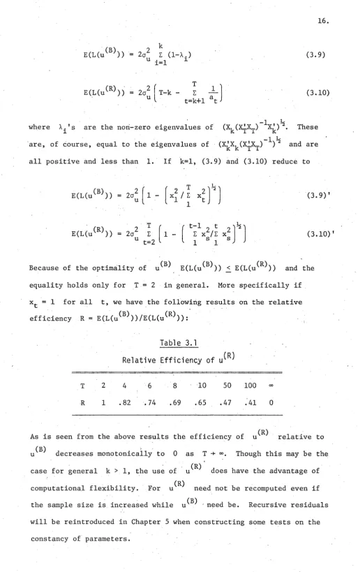
Because of the optimality of u^B ^ E(L(u^B^)) <_ E(L(u^B ^)) and the equality holds only for T = 2 in general. More specifically if x = 1 for all t, we have the following results on the relative

efficiency R = E(L(u^B^))/E(L(u^R ^ ) ) :

Table 3.1

Relative Efficiency of u ^

T 2 4 6 8 10 50 100

R 1 .82 .74 .69 .65 .47 .41 0

relative to (R)

As is seen from the above results the efficiency of u

u

(R)

case for general k > 1, the use of u

(R)

does have the advantage of computational flexibility. For u

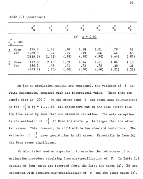
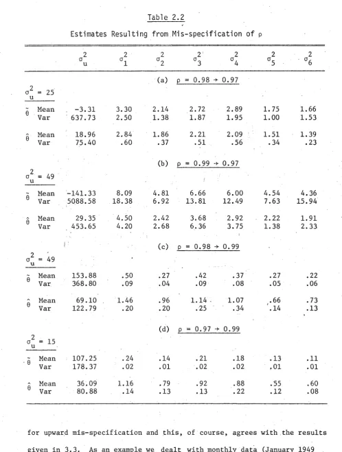
So far recursive estimation has been restricted to the one

developed by. Plackett (1950), which is the equation (3.4) governed by

the additional equation (3.5). Here we disregard the equation (3.5)

and consider a recursion of the form

h = h - l + h t (yt ' ’ (t = ) (3.11)

where h^ is a kxl known vector and the recursion starts with an

arbitrarily fixed vector 3 . The study of the asymptotic behaviour of

this recursion is difficult for k > 1. Here we consider only the case

for k = 1. The following lemma seems to be useful for the study of

convergence.

LEMMA 3.1.

a t = k ta t-l + £t ’ (t = ) (3.12)

converges to 0 as t if

(i) k fc is bounded for all t and there exists tQ such that

t

11 k s = a t 1 0 ; s=t

o

00

(ii) ' E £ < 00 .

t=l

P r o o f .

f t

_f

n k a + E n k.

i s

v s=l ; ° S = 1 ^ i=s+l

3

f

1

1

= n k_T) a + E n k.

r—

1

II

W c

Cß II _{^ i=s+l}

3 >

£ 4- a

s t

t E s=t

£ /a

s s

t

Now it is seen that the first two terms converge to 0 since IT k -* 0

I S

s—1

and £g is bounded. On the other hand by virtue of (i) b fc = 1/a^

t t

a E i / a = E b £ /t> -> 0 as t -> 00 because of (ii) and

t s s ^ s s t

s=t s=t

o o

K r o n e c k e r ’s lemma (Gihman and Skorohod (1974), p.71).

The above lemma also holds if a and £ fc are random variables.

For that case by convergence should be meant the almost sure (a.s.)

convergence. As to the convergence of the recursion (3.11) for k = 1

we have

Theorem

8 as t if

(i)

(ii)

k = 1 - trx^ is bounded for all t and there exists t

t t t o

t

such that II k = a. 1 0 ;

. s t

s=t

o 00

E h 2 < * .

t=l Ü

P r o o f .

(3.11)

a

t V t - l + V t

where c*t = ß - ß and the recursion starts with arbitrarily fixed a Q .

Then we can get the conclusion by virtue of the above lemma if

00

E h u < 00 (a.s.). This is really ensured since {h^u^} (t = 1,2,...)

t=l 1

is a sequence of independent random variables with

OO OO

2 2

E Var(h^u^) = a E h < 00 by (ii) so that Kolmogorov's theorem

t=i 1 u t=i c

(Gihman and Skorohod (1974), p.67) applies.

Theorem 3 . 2 .

3.1 ß

converges in mean square (m.s.) to ß as t 00.

2 2

(1) If h = x / E x and E x -* °°, then the conditions (i) and

t t , s . s

s=l s=l

(ii) in Theorem 3.1 are necessarily satisfied. For 0 < 1-h xt _< 1 for all t _> 2, which implies (i) and (ii) is ensured by the fact that

Vi

t=l

E x s=l S

for a > 1 if E x s=l *

(3.13)

In this case Theorem 3.1 gives an alternative proof for the theorem due to Anderson and Taylor (1976).

(2) Two sets of conditions which seem more plausible but stronger than

the conditions in Theorem 3.1 are

(i)'

(ii)T

(i) holds;

■ t = x t /

t E x

i s s=l

(a > and E x -> °° ; i s

s=l and

(i)"

h t “ xt

/

r t ? \a

t

(h < a < 1) and E x 00 ; E x.

s=l s—1

(ii)" h tx t + 0 .

That (ii)1 -> (ii) is obvious from (3.13). On the other hand from the inequality

t

n

s=l

t

- E h x for . 0 < h x < 1 , — s s —

it is seen that the condition (i) is satisfied if diverges to 00

and h txt i 0* The former is implied by (i)" and the latter is just the condition (ii)". On the other hand (ii) holds because of (i)".

2, 2, \ \ h

(3) If lim Ext/t remains bounded and | x^. | <_ t for t > t , then

we can put h t = x^/t. It is easily checked that this satisfies the

Finally we mention some possible applications of the Kalman filter

or Plackett’s algorithm. These are:

(i) detection of the parameter change over time;

(ii) detection of the parameter change over the frequency bands;

(iii) estimation of the coefficient parameters for time series

models.

C H A P T E R 2

T HE I D E N T I F I C A T I O N P R O B L E M IN T IM E V A R Y I N G P A R A M E T E R M OD EL S

2.1

I n t r o d u c t i o n

In Chapter 1 we discussed how to estimate Bt in the time varying parameter model:

y t = + u

Bt = Fßt_ 1 + et , (t = 1 .... T)

(1.1)

assuming that the parameters o = Var(ut), E = Cov(et), and F are all known. In practical situations they are either unknown or known only approximately. Then it is necessary to estimate these parameters. However, and here the situation is different from the usual linear regression model, it is not obvious that these parameters are estimable or identifiable. Let 0 be the set of possible parameters 0 which is

£

a set of K-dimensional Euclidean space R and 0q the true parameter value in 0. Also let £(0) be the likelihood function based on a sample of size T. Then by the identifiability of 0q ^ 0 we mean that

£(0) = £(0q) (a.s.) =► 0 = 0q (1.2)

where the measure is taken with respect to the true distribution. This definition of identifiability is concerned with all 0 in 0 and we shall speak of global identification in this case. On the other hand if (1.2) holds in some open neighbourhood of 0q , 0q is said to be locally identifiable. As is clear from the definition, a knowledge of the distribution of the sample is needed. Throughout this chapter we deal explicitly with the case where the distribution is normal.

However, the above criteria for identifiability are usually

I

*(e„)

I(6|0O ) = I £(0o )log w dyr ..dyT = 0 - 0 - 6q (1.3)

where we assume that the integral is meaningful. 1 ( 0 16Q) is called

Kullback’s information integral. It is noted that 1 ( 0 |0 ) is always

non-negative and that identifiability is concerned with finding a unique solution to the minimum of 1 ( 0 | 0q ) , that is, 1 ( 0 |0 ) = 0. Notice also that 1(0 100 ) = E{log £(0q ) “ log £(0)} and thus we may say that the

parameter 0q is identified if and only if E{log £(0)} attains a

unique maximum at 0 = 0 . The function 1 ( 0 |0Q ) can be used as a

criterion for discriminating £(0 ) against £(0). The so-called

Akaike’s information criterion (AIC) (see Akaike (1973)) was derived

using this property of I (0|0q ). In any case following the criterion

(1.3) it is easily shown that the parameter 3 in the usual, normal

linear regression model is globally identifiable if = (x-^,...x^)

is of full rank as expected.

On the other hand as far as local identification is concerned, it has been shown in Rothenberg (1971) that, under some regularity condi­

tions, the local identifiability of 0q is equivalent to the positive

definiteness of the information matrix:

W

E

' a

30 30’

0=0

(1.4)

Note that 11^(0^) = (3^1(0|0 )/3630’)q_q under the regularity

condi-o

tions and that H,j,(0o ) depends only on the true parameter 0q . Bowden

(1973) points out that the condition (1.4) can be derived as a simple

corollary to (1.3). In terms of the information matrix Rothenberg

(1971) also considers global identification. His result is that every

parameter 0 in 0 is globally identifiable if £(0) belongs to the

Following this criterion we get the same identifiability condition as above for the parameter 3 in the normal linear regression model since

HT (ß) = Xptj/o^.

So far we have restricted ourselves to the case where the sample

size T is finite. In connection with inference problems the case where

T

’asymptotic identifiability', the definition of which is given by I

lim(L(0)/dT) = lim(L(0 )/d ) (a.s.) =► 0 = 6 (1.5)

T-K» T-x» ° °

where L(0) = log £/(0) and d^ is a positive number such that d^ °°

as T -* 00. The criterion similar to (1.3) is

lim(I(0 I 0 )/d ) = 0 =* 0 = 0 . (1.6)

T-x» o i o

As noted below (1.3) 0^ is asymptotically, globally identifiable if

and only if lim(E(L(0))/d~) attains a unique maximum at 0 = 0 .

T-x» °

Considering again the parameter 3 in the normal linear regression

model it is asymptotically, globally identifiable if X^X^/d^ Q > 0.

In this case the normalizing factor dT is usually taken as T. Moreover asymptotic, local identifiability can be checked by

lim(H (8 )/dT) = H(0 ) > 0 .

(1.7)

The identification problem in time varying parameter models was

initially considered in Cooley and Wall (1978). Using a more general

Here we consider the identification problem independently of their work since our model is different and we are mainly concerned with asymptotic identifiability.

In Section 2 we consider the case where y^_ is stationary with an

absolutely continuous spectrum. Although this may be very special, this

case becomes important when constructing stationary signal plus noise

models in Chapter 4. In Section 3 a general case is considered for

finite T where the matrix F is assumed to be the identity matrix.

Asymptotic identification is considered in Section 4 using the same model

as in Section 3. Only some partial results are given to this problem

since it is not easy to give a complete answer as far as the author's present knowledge is concerned.

2.2 I dentifiabi1ity for Stationary Cases

In this section we deal with the asymptotic identifiability of the

true parameter 0q assuming that y fc is stationary in the wide sense

with the autocovariance function y(r) = Cov(y ,y + ) (r = 0, + l,...).

It is necessary that E (31) = 0 for all t since E(yt) = x^.E(ßt);

otherwise E(yt) is not constant for all t. Then it is known that

there exists a uniquely defined non-decreasing function F(u)) ( -it <_ w <_ it) with F(-tt) = 0, F (tt) = y(0), and continuous on the right ( -it' < w < tt) such that

Y(r)

r-n

iroo

e dF (to)

J -TT

(r = 0 , + 1,...) (2.1)

where the integral is a Lebesgue-Stieltj es integral and F(m) is called

F(ü>) = F 1 (o)) + F 2 (üj) + F 3(oj) (2.2)

where F^Coo) is absolutely continuous, F 2 (w) is a step function con­

taining at most a countable number of finite jumps, and F 3(m) is con­

tinuous and may be increasing although dF3 (to)/dw = 0 (a.e.). In

practice F^Coo) may be disregarded. In the subsequent discussions we

assume that F(w) itself is absolutely continuous so that dF(m) = f(w)dw.

The function f(w) is called the spectral density or simply the spectrum

of y . A sufficient condition for F(w) to be absolutely continuous

is that y(r) is absolutely summable, that is

oo

E Iy(r) I < oo . (2.3)

£• = — OO

This assumption seems reasonable with the present model (1.1) since

y(r) is expected to decrease exponentially with r. Thus (2.3) is also

assumed and then we have

OO

f (to) = -rt E y(r)e-lra’ (2.4)

— — CO

which is continuous under the assumption (2.3). Note that .f(w) is

always non-negative and even. To express the dependence of f(w) on

the parameter 0 we change its notation to f(o),0).

We have so far assumed that y fc is a zero-mean stationary process

with an absolutely summable autocovariance sequence (y(r); r=0,+l,. ..}.

As explained in Section 1 we also assume that y is Gaussian. Since

we are concerned here with asymptotic identification, the sample size

T is assumed to be quite large. Under such a circumstance, as pointed

out in Walker (1964), if f(w,0) is continuous and positive for all co

in [ —7T,7T] , the log-likelihood L(0) for any 0 in 0 can be

fU

L(0) = ■ tlog 2nf(m.0) + 7 ^ ) - ) d<0 (a.s.) (2.5)

• — TT

where I(oo)

T 2

5 y e

I

/ (2

T) .

t=l

To give an asymptotic, global

identifiability theorem we also require the process to be ergodic (see

Hannan (1970, p.201) both for the definition and for the justification

of this assumption). Of course y becomes ergodic in the present case

if u t and e are both Gaussian. Under the ergodicity assumption

Hannan and Robinson (1973) have shown that if g(w) is a continuous

function of oo with period 2t t, then

r TT

lim g (a)) I (oo) do) =

T-*x> J -u

The proof of this statement will be given in Chapter 3 when we prove

central limit theorems for spectral estimators. By virtue of this

result L(0) in (2.5) can further be written as

g(ui)f (a), 0o )do) (a.s.) (2.6)

“ IT

lim(-2L(0)/T) T-*»

(log 2Trf(o),0) +

f (a),0Q )

f (oo, 0) doo \ (a.s.). (2.7)

It is also known that if f(o),0) is positive and continuous for all w

in [ — it,tt] , y t has a unique one-sided moving average representation:

and thus

yt a,(0)e

3=o

2

E a . (0) < « , aQ (0) = 1

j=o J

f (a»,0) o

2(6)

2tt E a.(0)eljw

j = o J

(

2

8

Here a sequence of independently distributed normal variables

2

The major reference here is Hannan (1970, p.159).

T h e o r e m

f (to, 0) = f (to, 0q) (a.e.) => e = 0q

.

P r o o f .

minimum at 0 = 0 if and only if the condition described in the theorem

o

2

holds. Since a (0) is the prediction variance of a stationary process

with the spectrum (2.8), it holds that

log o (0)

JL_

2tt

J

-l o g 2ttf ( t o , 0 ) dm (2.9)

Note that the integral in (2.9) is well defined because f(io,0) is

continuous and positive for all oo in [ —tt ,tt] . On the other hand we

have

o

2(8)

f (u>,90 )

f(u,0)

dw

since the right hand side is the variance of a process with the spectrum

f (to, 0q ) / (2iTf (to, 0)) (see the formula (2.1)) and this is not smaller than

2 2

its prediction variance o (0 )/a (0) (see the formula (2.8)). The

equality holds if and only if

f(to,0 ) o 2 (0 )

’ o _ o'

f(“’9) ” a2(0)

(2.11)

[TT f ( u ) » e ) ~ (0 )

—

2

f (o), 6)

— ^r-} doü

+ — ---

(2.12)

2,1 J-n £(“ ’0) ~ o2(0)

w ith equality if and only if (2.11) holds. Moreover, using the

inequality log x + c / x 1 + log c (c > 0) with equality only when

x = c, we have

?

a2(e )

,

log a (6) + ■ i 1 + log a (6 ) . (2.13)

a (0) °

The equality holds if and only if o2 (e) a (0O ). Therefore

min

0 2*

{log 2irf(a),0) +

J - n

f (w,0Q )

f (a>,0) } doo 1 + log a (0q ) (2.14)

2 2

and the minimum is attained if and only if both (2.11) and a (0) = a (0Q )

hold. Since f(oo,0) can be expressed as in (2.8), we must have the

condition described in the theorem, which completes the proof.

Because of this result we can check the asymptotic, global

identifiability of the parameter 0q in terms of the spectral density.

The parameter 0q will be asymptotically, globally identifiable if

there exist no other 0 in 0 which give rise to f(w,0) = f(o),0Q )

(a.e.). It may be noted that the uniqueness of f(w,0) at 0 = 0q

is a conventional identifiability criterion adopted in time series

analysis. Since there exists a one-to-one correspondence between the

spectrum and the autocovariance sequence, we may say that 0^ is

identifiable if the latter is uniquely determined. For illustration we

consider some simple models to see if the parameters in those models are

(i) Case I

Consider the simplest model

yt = et + ut

(2.15) ß t = P ß t _ 1 + e t > P + °> i PI < 1

2 2

where all variables are scalar. Put 0 = (a , o , p)'.

u e Then we have

r 2

p

°e

2

y(r) = - - - + 5 a

' , 2 or u

1 - P

f (u),0) 2tt

1 - pe

e . 2

— ;-- ~ + o

leu I 2 u

Now it is almost obvious that f(co,0) is unique at 0 = 0^ (see Hannan

(1970), p.171). The assumption that p 0 and |p| < 1 is

indispen-2 2

sable. If p = 0, y t itself is white noise and f(oo,0) = (a + g u)/2tt

2 2

so that we cannot determine ö£ and a uniquely. On the other hand

if Ip j >_ 1, y is not stationary any more and thus p must be less

than 1 in modulus. This may also be justified in terms of f(w,0)

since there always exists

9

=

(V G

e

^p2

’ 1/,p^

'

such that f(w,0) = f(u),0Q ).

(ii) Case II

Consider another special model (1.1) with

x^ = (cos X,t, sin X,t,...,cos X t, sin X t ) '

t 1 1 s ’ s ; 2sxl

F = diag(p1 ,p1 ,...,ps ,ps ) ; 2sx2s (2.16)

w h e r e A_. =j= A^ (mod 2ir) a n d if A^ = nir (n; integer), sin A_.t w i l l

be s u p p r e s s e d f r o m the m o d e l t ogether w i t h c o r r e s p o n d i n g e l e m e n t s in F

and E. This m o d e l seems u s e f u l if the d a t a c o n t a i n s p e r i o d i c i t i e s

2tt/A_. (j = l,...,s). E s p e c i a l l y if the d a t a is monthly, w e m a y put

\

and w e s hall d e a l w i t h this case m o r e c l o s e l y in C h a p t e r 4. Put

2 2 2

9 = (ou ,a1,...,ög, p1,...,p)'. N o w w e h a v e

y(r) s

Z

j=l 1-P

i 2

, cos A .r + 6 a

: j or u (2.17)

so that, f o l l o w i n g the d e f i n i t i o n of f(m,0) in (2.4), it is not h ard

to d e r i v e

f (a), 0 )

1-p . e J

i(o)-A^) 2 +

1-p . e J

i(m+Aj)

To i d e n t i f y the p a r a m e t e r 0q it is m o r e c o n v e n i e n t in the p r e s e n t

case to use

y(r)

r 2 2

o b s e r v e p 'a./(1-p.) for e a c h j and r > 0 so that p.'s can be

J J J J

2 2

i d e n t i f i e d first and thus a . 's can a l s o be identified. F i n a l l y a

J u

can be d e t e r m i n e d p u t t i n g r = 0.

(iii) Case III

This i l l u s t r a t e s a c ase w h e r e the p a r a m e t e r 0q is n ot identifiable.

C o n s i d e r a t i m e - i n v a r i a n t s y s t e m

y t = h'et + ut

3 = F3 _ + e

pt p t-l t

(2.19)

y(r) h ’ Z FJ ZF

j=°

j + |r

h + 6 o 2

or u

f(U ,9) = i h'( I k - F e lü))

-1

2 (Ik - F e 1U)) *

-1

h +

2tt

where A is the complex conjugate transpose of a matrix A. From a

different point of view Mehra (1970) has shown that Z cannot be

identified if the number of unknown parameters in Z is greater than k

even if F is known; otherwise there is a possibility that Z can be

identified. Thus if Z is positive definite and there exists no a priori

restriction on Z, Z is not identifiable. As an illustration consider a

simple case where F = pl^. Then it is seen that h ’Z^h = h ’Z2h does

2

not necessarily imply Z^ = Z2 . Note that in this simple case and

p are identifiable.

The following case deals with a somewhat different situation. So

far we have discussed the case where y is Gaussian and stationary.

The process y^ becomes Gaussian if u and e are both Gaussian

since x._ is assumed to be non-stochastic. However if x^. is

stochastic, the distribution of y t is far from Gaussian though y

may be still stationary. Then the above theorem cannot be applied

directly to this case. Therefore it should be understood that the

identification result described below is the one based on a knowledge of

the spectrum of y fc or its autocovariance sequence and has no relation

to our identifiability criterion.

(iv) Case IV

In this case we assume that x^ is stochastic and consider a simple

model

X t3t + U t

Pß_{t-1 + £t ’} + < 1

where all variables are scalar. Let us assume that is mutually

independent of u^ and and is stationary with an absolutely con­

tinuous spectrum fx (u)) • Then we have

r 2

p °e 2

y(r) = Cov(x.,x. ) ---- + 6 o

' v t t+r ^ 2 or u

1-p

f (a), 0 ) fx (a.-A)fg (A)dA + ± o 2u

2

2

where 0 = (a , o , p)', f (w) is the spectrum of ß , and we have

U £ p t

assumed that Cov(x .x,. ) and thus f (w) are known. If x t is

t t+r x t

white noise, then the parameter 0^ cannot be identified as is easily

seen. On the other hand if Cov(x ,x^. ) is not zero for at least

t t+r

I r I 2 2

two r(> 0), then p 1 ‘a /(1-p ) is observable for these r. Hence p

e

2 . 2 ...

is identified and thus a is also identified. Hence a is identified,

e u

For example if x follows an autoregressive process

2 2

say with mean 0 and variance o f (1-a ), we have

axt-i + v

r 2 r 2

a 1 1 a p 1 ' a _

/ ^ v e , P 2

y (r) = ---- 5— ----— + 6 a

2 . 2 or u

1-c 1-p'

f (a), 0)

2 2

0 0 nt

v e 1

/ 2 J I i(ü)-X) 12 I

4tt j -it 1-ae 1-pe

. ■> , 1 2

— — r- dA + — O

lX 1 2 2tt u

2 2 o a

v e ,1-a p2 2

2 2.

1-ape (1-a )(1-p )

1 2

+ -y— P

2tt u

and thus 0 is identifiable if a and o are known. As explained

o v

before we need some care when we deal with this case in connection with

estimation problems since y t is far from Gaussian even if the other

random variables are Gaussian.

not consider local identifiability defined in (1.7). Nonetheless it is

of some interest to see under what conditions (1.7) holds. To do this

we assume that f(oo,0) is twice continuously differentiable with

respect to 0 and that the resulting derivatives are also continuous

in a). Now it is seen from (2.7) that

9L(0) m T If7T 1 9f (o),0) f (a), 0q ) 9f(co,0)

' dto (a

Q J C D 1 1 4 > | =3 1

1 _=i f (u),6) 90 _{f 2 (u,0)} 90

92L(0) ip 'TT 1 9f (ü j, 0) 9 f( w, 0) r _o f ( w ' , 0 )_{° i}

9090' 4tt

' - 7 T _{. f 2 ( u , e )} 90 90' l " f (cu, e ) J

a2f (co,9) f f(t0’9o ) 1

3 0 3 0 ’ l f 2 (M ,e) " f(“ >0)

dm (a.s.) .

Therefore we have

lim T-x»

1 3 2l ( 0o> ] 1

r

9 f (oo ,0 )

o 9 f (a) ,0 )o T 3 0 9 0 ’ 4 t t

o C D 3 ■ w ' C N J c w t=

1 90 30'

doo (a.s.). (2.21)

We note that the matrix integral on the right hand side of (2.21) is

necessarily positive definite if the parameter 0q is asymptotically,

globally identifiable and some regularity conditions are satisfied. For

if 0q is asymptotically, globally identifiable, 0q gives a unique

maximum of lim E(L(0)/T). Therefore, under some regularity conditions,

T-x»

it must hold that

lim E

T-x»

1 3L <0O> 1

T 30 o

lim E

T-x»

JL T

92L(0 ) >> _____ o_

9090' < 0 .

On the other hand we want to find a necessary and sufficient con­

us consider

where x is a K><1 constant vector and x =j= 0. Then it is seen that

we must find a condition that

x' --- I dm > 0 for any x

9f (to, 0 ) a ^

00 j + o •

Since the components of 9f(co,0 )/90 are rational polynomials of to so

that x'9f(to,0 )/30 is also a rational polynomial, the above inequality

holds if and only if the components of 3f(to,0Q )/90 are, as functions

of to, linearly independent (a.e.) with respect to Lebesgue measure.

This is summarized in

T h e o r e m 2 . 2 .

spectrum f(to,0) which is positive for all to in [ -i t,it] . Also assume

that f (to, 0) , 9f(to,0)/30, and 92f (to, 0) / 90 90 ’ are continuous in to and

0. Then a necessary and sufficient condition for the parameter 0^ to

be asymptotically, locally identifiable is that the components of

9f(to,0 )/90 are, as functions of to, linearly independent (a.e.) with

respect to Lebesgue measure.

In general it is not easy to check if the above identiflability

condition is satisfied or not. This is mainly because F is unknown.

Let us assume that F is known. Then the unknown parameter 0 is

2

composed of and E. Moreover the spectrum f(to,0) becomes linear

in 0 and can be expressed as

f(m,0) 9f (to,0)

(

.

)

_, . 1 ^ ✓ v -irw f (w ’0) = 2tt e y (r )e

r=-oo and

y(r) = x' £ (FJ E F ,J)F'Sc + 6 q

t . t+r or u

J = o

Hence global and local identiflability conditions are equivalent in the present case as is easily seen.

2 . 3

I d e n t i f i a b i 1 i t y f o r N o n - S t a t i o n a r y C a s e s W h e n T is F i n i t e

Throughout the present and next sections we consider local

identification for non-stationary cases. In this section the case where

the sample size T is finite and fixed is discussed. To reduce the

complexity of the problem we assume that the matrix F in (1.1) i s 'the

identity matrix of kxk. We start by describing the likelihood function

based on a sample of size T. To do this we assume that the initial

value 30 is also an unknown parameter to be identified. Now expressing

y in (1.1) in terms of 3 we have

t o

x'$ + x ’ Z e + u

t o t s t

s=l

(t = 1,...,T) (3.1)

or equivalently

where

y = X3 + v

y (yi> • • • ,yT) j x (x^,... ,x,j,) ,

and

X

f N

e.

Ul I

1 1 1

0

x 2 X 2 e2 u 2

•

•

+ •

X T XT * * * XT _{£T j} tu,