A d a p tiv e Echo C an cellation in
T elecom m u n ication s
John Homer
BSc (Hons I), University of Newcastle
April 1994
A thesis submitted for the degree of Doctor of Philosophy
of the Australian National University
Department of Systems Engineering
D eclaration:
The contents of this thesis are the results of original research, and have not been submitted for a higher degree at any other university or institution.
A number of papers resulting from this work have been submitted to or are under preparation for submission to refereed journals:
[JS1] John Homer, Iven Mareels and Robert Bitmead, “Analysis and Control of the Signal Dependent Performance of Adaptive Echo Cancellers in 4-Wire Loop Telephony” , accepted for publication, I.E.E.E. Transactions on Circuits and Systems.
JS2] John Homer, Robert Bitmead and Iven Mareels, “Quantifying the Effects of Dimension on the Convergence Rate of the LMS Adaptive FIR Estimator” , submitted for publication, I.E.E.E. Transactions on Information Theory.
[JS3] John Homer and Iven Mareels, “Echo Canceller Performance Analysis in 4-Wire Loop Systems with Correlated AR Subscriber Signals”, accepted for publication,
I.E.E.E. Transactions on Information Theory.
[JS4 John Homer, Bo Wahlberg, Iven Mareels and Fredrik Gustafsson, “Adaptive Detection and Estimation for Acoustic Echo Cancellation” , under preparation.
A number of papers have been presented at or have been submitted to conferences. Some of the material covered in these papers overlaps with that covered in the pub lications listed above:
[Cl] John Homer, Iven Mareels and Robert Bitmead, “Signal Dependent Perfor mance of Echo Cancellers” , Proceedings of International Symposium on Adaptive Systems in Control and Signal Processing (A C A SP ’92), 1-3 July 1992, Greno ble, France, pp. 621-626.
[C3] John Homer and Robert Bitmead, “Effects of Dimension on LMS Adaptive Filter Dynamics” , Proceedings of European Control Conference (ECC’93), 28 June-1 July 1993, Groningen, The Netherlands, pp. 2203-2206.
[C4] John Homer, “Curse of Dimension on the Learning Rate of the LMS Adaptive FIR Filter” , Proceedings of International Conference on Acoustic, Speech and Signal Processing (ICASSP’94), 19-22 April 1994, Adelaide, Australia, Vol III pp. 405-408.
[C5] John Homer, Bo Wahlberg, Fredrik Gustafsson, Iven Mareels and Robert Bit- mead, “LMS Estimation of Sparsely Parametrized Channels via Structure De tection” , submitted to IEEE Conference on Decision and Control (CDC ’94).
The work described in this thesis has been carried out in collaboration with a number of people. They are: Dr Robert R. Bitmead, Dr Iven M.Y. Mareels, Professor Bo Wahlberg and Dr Fredrik Gustafsson. However, the majority of the work is my own. April 28, 1994
A ck n ow led g em en ts
I owe a great deal of thanks to my supervisors Bob Bitmead and Iven Mareels. They make a great supervisory team, having an incredible knack for steering the research into directions of fruition as well as providing heuristic insight and assistance with problems at hand.
I am also very grateful for Bob and Iven’s encouragement. However, the greatest source of encouragement came from Kerry and for this I am very grateful. Without Kerry’s love and support I would be still struggling through the PhD studies. I am also very grateful to Kerry for helping me relax and enjoy my leisure time - an important part of the last three years. To the Homers and Bradburys, I am also grateful for their love and support.
I am very grateful to the friends I have made during my PhD studies, for the friend ship, support and good times they have given me.
I want to thank also Bo Wahlberg and Fredrik Gustafsson for working with me in the final stages of my PhD studies. The results of the research we carried out added significantly to my thesis. To Wolfgang Sauer, Vincent and Collette Wertz, Marc Moonen and Bob Stewart I am grateful for their hospitality and the opportunity they gave me to visit their respective Departments during my month long stay in Europe in 1993.
A b s t r a c t
The focus of this thesis is the suppression of echoes within speech transmission telecommunication networks via the LMS adaptive FIR echo canceller. Poor pe- formance of this technique has been reported, particularly when the required FIR tap length is large and the input signal is highly autocorrelated speech. The first aim of this thesis is to quantify the weaknesses of the LMS adaptive FIR filter, particularly the weaknesses relevant to echo cancellation. The second aim is to develop techniques which reduce the effects of these weaknesses and, consequently, enhance performance.
We begin with a brief review of alternatives to the LMS/FIR based echo canceller, wrhich emphasizes that such alternatives are, in many ways, inferior. We then carry out a rigorous dynamical analysis of the LMS adaptive FIR filter connected in parallel with an unknown channel. We consider the case in which the adaptation stepsize [i is
‘small’. The analyses focus on quantifying the adverse effects on transient performance of the autocorrelation level of the input signal and the filter parameter dimension (FIR tap length). The analytical results indicate conclusively that transient performance deteriorates with increasing filter dimension and input autocorrelation. A review of asymptotic analyses indicates that asymptotic performance also deteriorates with increasing filter dimension.
Dynamical analyses are then conducted on a system more representative of an echo cancellation network - a closed loop with an adaptive filter/unknown channel pair at each end and driven by signals entering from within the unknown channels. The analytical results indicate th at the (transient and asymptotic) performance generally deteriorates with increasing filter dimension, while it is improved by either whitening the driving signals or whitening the input signal to each adaptive filter/unknown channel.
signals) of the telecommunication network. The other assumes an autoregessive (AR) model of the input signals (typically used for speech) and whitens the input signals by filtering with AR estimates. To avoid distortion of received signals, indirect AR filtering methods are explored.
C o n ten ts
A ck n o w le d g e m en ts
A b stra ct
1 In tro d u ctio n
1.1 Echo Path Characteristics and Echo Canceller Requirements 1.1.1 Circuit E c h o e s ... 1.1.2 Acoustic Echoes ... 1.2 Motivation for Research and Thesis A pproach... 1.3 Thesis Outline ... 1.4 Summary of Original C ontributions...
2 A d a p tiv e F ilterin g and E cho C an cellation - A R ev iew
2.1 In tro d u ctio n ... 2.2 LMS adaptive FIR f i l t e r ... 2.2.1 Input Signal Autocorrelation E ffe c ts ... 2.2.2 Effect of Input Signal Pow er... 2.2.3 Effect of FIR Tap L e n g t h ...
2.3 NLMS Adaptive A lg o rith m ... 2.4 RLS A lg o rith m ...
iii
iv
1
4 4
6
8
10
12
14
2.5 Lattice Filters 21
2.6 IIR F ilte rs ... 21
2.7 Frequency Domain F ilterin g ... 24
2.8 Sub-Band F ilte rin g ... 26
2.9 Adaptive Filtering for Echo Cancellation... 28
2.10 Conclusion ... 32
Chapter 2 Appendix: Remarks on Double T a l k ... 34
3 Q u a n tita tiv e A n a ly sis o f th e LMS A d a p tiv e F IR F ilter 35 3.1 Introduction... 35
3.2 System D escription... 37
3.3 Review of Transient Performance Analyses... 40
3.4 Averaged System E q u a tio n s... 43
3.5 Convergence Cost F u n c tio n ... 44
3.6 Cost Function A nalysis... 46
3.6.1 Analysis for Autoregressive Input S ig n a ls ... 48
3.7 Asymptotic Performance Analysis ... 55
3.8 Conclusion ... 59
Chapter 3 Appendix: Averaging Error A n aly sis... 61
4 A n a ly sis o f th e L M S /F IR F ilter in C losed Loop E cho C a n cella tio n 71 4.1 Introduction... 71
4.2 Heuristics and Literature R e v ie w ... 73
4.3 System E quations... 74
4.5 Analysis of Single Tap Echo Paths/Cancellers 80
4.5.1 System Equations ... 81
4.5.2 Domain of Analysis ... 81
4.5.3 Averaged Residual Echo Parameter Update E q u a tio n s... 83
4.5.4 Zero Cross Correlation A nalysis... 84
4.5.5 Nonzero Cross Correlation ( Noise Absent) ... 88
4.5.6 S im u latio n s... 93
4.5.7 S u m m ary ... 94
4.6 Single Tap Single Delay DEC System with AR Subscriber Signals . . . 94
4.6.1 A s s u m p tio n s ... 95
4.6.2 A n a ly sis... 97
•4.6.3 Subscriber Signals of Unequal P o w e r...100
4.7 Conclusion ... 103
5 S ig n a l C o n d itio n in g for E ch o C a n c e lle r s 108 5.1 Introduction... 108
5.2 Signal Conditioning with Digital Scram blers... 110
5.2.1 Scramblers ...110
5.2.2 Signal Scrambling ... I l l 5.2.3 Scrambler Scheme for Echo C ancellation... 116
5.2.4 S im u latio n s... 118
5.3 Signal Conditioning via Autoregressive Filtering ... 119
5.3.1 AR Based Whitening Schemes ... 120
5.3.2 D iscussion... 125
6 D im e n sio n R ed u ced L M S /F IR E stim a tio n 130
6.1 Introduction... 130
6.2 Echo Path Structures ... 132
6.3 System D escription...134
6.4 Requirements and Benefits of Active Tap P aram etrizatio n ... 135
6.5 Active Tap D etection...137
6.6 LMS Estimation via Detection ... 144
6.7 Conclusion ... 147
7 C o n clu sion s and Future W ork 150 7.1 C onclusions... 150
7.2 Future Directions of R esearch ... 153
7.2.1 Dynamical A n a ly s e s ... 153
7.2.2 Signal Conditioning S c h e m e s ... 154
7.2.3 Dimension Reduced LMS/FIR E stim atio n ... 154
7.2.4 Nonlinear Effects in C h an n els... 155
A P re lim in a r y C on cep ts 156 A .l Order Function and 0 (.) F u n c tio n ... 156
A.2 Time Scale ... 156
A.3 Lipschitz C o n tin u ity ...157
A.4 Uniform C o n tra ctio n ...157
B T h e A veragin g M eth o d 159
C R ecu rsiv e Least Squares 161
E R e m o v in g M e a s u r e m e n t N o is e E ffe c ts - S p a rse C h a n n e l I m p u ls e R e
s p o n s e E s t im a t io n 166
F C h a p te r 3 P r o o fs 168
F .l Proof of Theorem 1 ... 168
F.2 Proof of Theorem 2 ...169
F.3 Proof of Lemma 1 ... 170
F.4 Proof of Theorem 3 ...171
F.5 Proof of Theorem 4 ...172
F.6 Proof of Theorem 5 ...176
F. 7 Proof of Theorem 6 ... 177
G C h a p te r 4 P r o o fs 179 G . l Proof of ( 4 . 2 7 ) ...179
G.2 Proof of Theorem 7 ... 180
G.3 Proof of Theorem 8 ...181
G.4 Proof of Theorem 9 ...182
G.4.1 Constructing the Lyapunov Equation ... 184
G.4.2 Maple procedures to solve a Lyapunov equation...185
H P r o o f o f L e m m a 2 188
I L ist o f A s s u m p t io n s 189
C h ap ter 1
In tro d u ctio n
An echo, in any context, is a delayed and perhaps distorted version of a previously transm itted signal. In telecommunication systems, the occurrence of echoes tends to reduce quality of transmission. In data transmission, echoes of sufficient magnitude result in an increase in error rates and may lead to retransmission being required. In speech transmission, the perceived quality reduction depends on the echo delay as well as the magnitude (and spectral distortion) [1]. In particular, if the echo delay is sufficiently short ( ss 10ms) then the echo is not noticeable and for this reason echo problems in speech transmission, in the past, were only encountered in international calls [1], particularly with satellite systems. The introduction and growing use of digital processing in speech transmission, however, has lead to the occurrence of delays in national networks comparable w'ith those of international networks [2]. The occurrence of echoes with the potential to disrupt telephone conversations, and the need for echo suppression techniques has consequently grown considerably.
attenuation device in each direction of transmission. Due to the nature of echo gen eration, this causes the echoes to be attenuated twice as much as the transmitted signals. This approach, however, causes unsatisfactorily low signal levels at the re ceiver for circuits longer than about 3000km [1]. A more sophisticated approach is to insert an attenuation device into the receiving or transmitting circuit according to which is least active. In speech transmission systems, this approach is known as voiced controlled switching. It was very popular for controlling circuit echoes [1], [2], [13], [6] and is currently the most commonly used technique for acoustic echo control [20], [6]. A major drawback of this technique is that during full duplex transmission - that is simultaneous transmission by the subscribers at both ends of the network - one of the transm itted signals is necessarily attenuated.
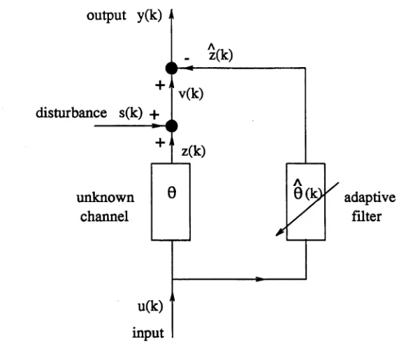
A popular alternative is that of echo cancellation which is illustrated in - Figure 1.1. This technique involves connecting a digital filter, the echo canceller, next to and in parallel with the echo source or echo path. The echo canceller samples the signal u(k)
feeding the echo path and, if correctly designed, outputs a signal z ( k) which replicates the echo z(k). This echo replica is then subtracted from the echo containing signal
v(k). To enable suppression of echoes generated by time varying echo paths, the echo canceller is typically adaptive. The use of adaptation also allows, to some extent, the echo canceller to be given arbitrary initial conditions, and thus reduces the costs due to initial echo path measuring.
transmit
Subscriber
receive
s(k) + v(k) + _ y(k)
n + z(k)
Echo
Path
z(k)
Echo Canceller
u(k)
Figure 1.1: Echo suppression via echo cancellation.
The popularity of echo cancellation as a means of suppressing echoes in telecommu nication networks mainly is due to its parallel configuration which leads to:
[image:13.521.106.369.463.599.2]Of course, once the transients have died out, adaptive echo cancellation also leads to negligible distortion/attenuation of the transmitted subscriber signals.
The basic requirements of an adaptive echo canceller are:
• rapid suppression of echoes or, in other words, good transient and asymptotic performance;
• low computational complexity.
Usually, there is a trade-off between these two objectives. The meeting of these two objectives depends on a suitable choice of the following design factors:
• filter structure; • adaptation algorithm.
Commercially made echo cancellers typically involve [3], [5], [6], [7] Finite Impulse Response (FIR.) filters and the Least Mean Square (LMS) adaptive algorithm (or the closely related Normalized LMS (NLMS) algorithm). The major advantages of this echo canceller type are those of relatively low computational complexity, good stability properties, relatively good robustness against implementation errors [8] and that its behaviour is relatively easy to understand. Importantly, in a great many cases this popular echo canceller type provides adequate echo suppression with low computational complexity.
In a bid to achieve better echo cancellation under a greater range of circumstances, alternative echo cancellers to the conventional LMS adaptive FIR filter type have been and are being considered. These involve:
• modifications of the LMS adaptive FIR filter
• different filter structures and/or adaptation algorithms.
A review of the various types of echo cancellers is presented in Chapter 2.
• The new techniques assume that the echo path is Linear.
• Echo cancellation in data transmission typically is required to suppress a small but important nonlinear component (-40dB relative to that of the Linear component) of the echo path. This nonlinear component, which is introduced by the circuit com ponents of the digital transceiver [9], can be usually ignored in speech transmission. In data transmission, however, it must be considered because of the need for greater echo suppression [26].
The outline of the remainder of this introductory chapter is as follows. In Section 1.1 we give an introduction to the causes of echo, a description of the echo path char acteristics and of the requirements of the echo canceller. We consider circuit echoes and acoustic echoes separately. In Section 1.2 we provide motivation for continued research into adaptive echo cancellation and for the approach taken in this thesis. An outline of the thesis is presented in Section 1.3 followed in Section 1.4 by a summary of our original contributions.
1.1
Echo P a th C h aracteristics and Echo C anceller R e
q u irem en ts
1 .1 .1 C i r c u i t E c h o e s
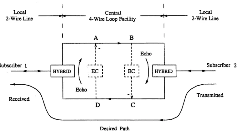
To understand how circuit echoes are generated and how they may be controlled consider the simplified telephone network of Figure 1.2. In this network the two subscribers are linked to a common central 4-wire loop facility via local subscriber 2- wire lines. The local 2-wire lines allow communication in either direction. In contrast, each of the 2-wire lines of the central 4-wire loop facility allow transmission in one direction only. Such unidirectional transmission enables the use of amplifiers and also of multiplexing i.e the sharing of one transmission channel by a number of calls. Generally, these advantages of unidirectional transmission are only necessary for long circuits and, consequently, for circuits shorter than about 60kms, the central 4-wire loop facility is not included [1].
Local ________ , ________ Central ________ , ________ Local
2-Wire Line 4-Wire Loop Facility 2-Wire Line
Subscriber 2 Subscriber 1
HYBRID HYBRID
Transmitted Received
Desired Path
Figure 1.2: Central 4-wire loop telephone network
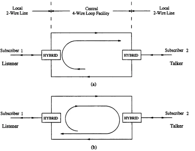
a circuit bridge, a balancing impedance which is set to match the input impedance of the connected 2-wire line. However, for multiplexing purposes, a hybrid may be connected to any one of a large number of different local 2-wire lines. Due to variations in the length, type and gauge of wire and number of phone extensions of the 2- wire lines connected [1] it is not economically possible to ensure perfect, or even near perfect, impedance matching [1], [2], [10]. As a result, the far end transmitted signal typically ‘leaks’ through the hybrid into the opposite 4-wire loop channel. This results in an echo being received by the far end (i.e. the original) subscriber - Figure 1.3a. Poorly terminated circuits may also lead to the receiving of echoes by the near end subscriber as indicated in Figure 1.3b and/or the observation of multiple echoes separated by time intervals equal to the round trip delay. It is important to add that because impedance matching of the distributed local 2-wire circuit is attempted with a lumped network, the echo is not just an attenuated, but a filtered version of the far end transm itted signal [1].
[image:16.521.91.471.81.290.2]Local 2-W ire Line
Central 4-W ire Loop Facility
Local 2-W ire Line
Subscriber 2 Subscriber 1
HYBRID HYBRID
Talker Listener
Subscriber 2 Subscriber 1
Talker Listener
HYBRID HYBRID
(b)
Figure 1.3: Echoes within the 4-wire loop telephone network: (a) speaker echo, (b) listener echo
Figure 1.2 is typically only 15-16ms long [14], [5], [1] with the first 10ms typically being zero or ‘flat’ [1],
Combining the above characteristics of the circuit echo path with the fact that an 8kHz sampling rate is typically used for telephone speech processing, then adequate suppression (40dB) of circuit echoes via the technique of echo cancellation (Figure 1.1) should be achieved by using a digital filter having an impulse response length of 128 taps. To ensure adequate echo suppression for most telephone calls, however, a tap length of 256 taps is suggested [14]. So as to allow the echo canceller to have arbitrary initial conditions, the echo canceller is made adaptive. Since the echo path is time invariant or, at worst, slowly time varying then the algorithm used to adapt the adaptive echo canceller does not need to have particularly good tracking characteristics.
1.1.2 A c o u s t ic E c h o e s
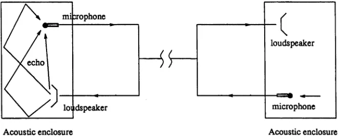
[image:17.521.88.403.80.324.2]sup-pressed. Each acoustic enclosure includes a loudspeaker for the receiving of signals transm itted from and a microphone for transmitting to the far end acoustic enclosure. The receiving of a signal at the loudspeaker results in, after some delay, an acoustic echo at the microphone via a direct path and paths involving reflections (on walls, furniture and persons). This acoustic coupling between loudspeaker and microphone is called the acoustic echo path.
mi :rophone
loi idspeaker
Acoustic enclosure
L f
L_
\ loudspeaker
)
microphone
Acoustic enclosure
Figure 1.4: The typical setup for hands free telephony or teleconferencing
Due to the relatively low speed of acoustic signals in air, acoustic echo paths tend to have relatively long impulse responses compared to electric echo paths. The at tenuation offered by acoustic echo paths is also relatively small. To be more specific: in hands free telephony, the impulse response is typically several tens of milliseconds while the attenuation may be 0dB or worse (that is amplifying rather than attenu ation) [15], [16]; in teleconferencing the impulse response length tends to be several hundred ms [15] [13], [17], [18], [19] and the attenuation 6-lOd.ö [15], [19]. Further more, CCITT recommendations for hands free telephony, indicate that the acoustic echo should be suppressed to at least 45dB below the level of the original speech [15], [2]. In the case of teleconferencing, where high audio quality is sought, similar if not greater suppression is required.
[image:18.521.103.434.196.332.2]A summary of the echo canceller requirements for suppression of circuit and acoustic echoes is given in Table 1.1.
Table 1.1: Echo Canceller requirements
Characteristic Circuit Acoustic
Sampling Rate 8 k H z 8 k H z, prefer 16 k H z
Impulse Response 200-300 200-4000 at (8k H z )
Tap Length 400-8000 at (16k H z )
Tracking Requirement Negligible Important
1.2
M o tiv a tio n for R esearch and T h esis A pproach
Adaptive echo cancellation based on the LMS (or NLMS) adaptive FIR filter is now the preferred method for suppressing circuit echoes in 4-wire loop telephony. Typi cally this approach yields relatively fast, essentially complete echo suppression with relatively low computational complexity. However, occasional poor performance such as signal bursting and/or slow, incomplete echo suppression has been observed [21], [22], [23], [24], [25]. To avoid such undesirable behaviour, there is a need to quantify the causes of such behaviour so as to enable the development of performance enhanc ing techniques for the LMS/NLMS adaptive FIR echo canceller or, alternatively, to motivate the use of more sophisticated echo cancelling techniques.
In contrast, the use of the LMS/NLMS adaptive FIR echo canceller for echo sup pression in acoustic telecommunication systems has not, in general, found a lot of success. This is due to the need for ‘long’ FIR filters in order to model acoustic echo paths adequately so as to achieve adequate asymptotic echo suppression. This requirement leads to high computational complexity and has been reported to lead to poor transient performance [20], [26], [27].
As a result of these problems, alternative echo cancelling techniques have been and are being examined. Most of these techniques, however, tend either to:
• improve transient performance at the expense of greatly increased computa tional complexity;
• reduce computational complexity but worsen transient performance;
To date, the acoustic echo cancellation techniques developed do not provide an im plement able ‘satisfactory’ solution [20], [4].
Possible directions for research into improving echo suppression within acoustic telecom munication systems include:
1. exploring alternatives to echo cancellation;
2. continuing to explore alternatives to LMS/NLMS adaptive FIR echo cancella tion;
3. developing performance enhancing techniques for LMS/NLMS adaptive FIR echo cancellation.
The first direction was the focus of research prior to the development of echo cancella tion. The more successful alternatives (see [20] for a greater range of such alternatives) and which are still in use today include: (a) voiced controlled switching and (b) studio environments with highly directional loudspeakers and microphones and sound ab sorbing materials [20]. There are obvious inadequacies with both of these alternatives. As mentioned previously, alternative (a), during periods of double talk, (i.e. speech is being transm itted by both acoustic enclosures) causes significant attenuation of one of the speech signals. On the other hand, alternative (b) is not very practical for most situations and, generally, requires minimal movement of the talker(s) in each acoustic enclosure.
The second possible direction of research is still the main focus of research today. The third approach, however, is that which we follow throughout this thesis. This decision is motivated by the following reasons.
• The LMS/NLMS adaptive FIR filter is the most popular adaptive estimation technique [8], [28] and, is likely to remain so in the foreseeable future.
• The dynamics of the LMS/NLMS adaptive FIR filter are relatively ‘simple’ and, generally, considerably simpler than those of the alternative echo canceller types. This may allow the ‘weaknesses’ of the LMS/NLMS adaptive FIR filter to be quantified through dynamical analysis and, in turn, enable possible performance enhancing modifications to be developed and analysed.
because, the adaptation stepsize, fi, used in practice is typically ‘small’ and under this condition, the LMS and NLMS algorithms show similar dynamical behaviour [29], [8]. Motivated by the above discussion, the aims of the work leading to this thesis have been as follows.
1. Through dynamical analysis attempt to quantify the weaknesses of the LMS adaptive FIR filter for the case in which the adaptation stepsize, //, is ‘small’. This needs to be carried out not only for the open loop case of Figure 1.5, in which we consider an isolated adaptive filter/unknown channel pair but also for the closed loop case of Figure 1.6 which is more representative of echo cancel lation networks.
2. Based on these weaknesses and the characteristics of echo cancellation networks, develop performance enhancing techniques for the LMS adaptive FIR echo can celler
disturbance s(k) + v(k) + output y(k)
adaptive filter unknown
channel
input u(k)
Figure 1.5: Open loop adaptive system - adaptive filter in parallel with unknown channel
1.3
T h esis O u tlin e
Chapter 2
[image:21.521.65.374.355.502.2]adaptive filters unknown
channel
unknown channel
Figure 1.6: Closed loop adaptive system - an adaptive filter/unknown channel pair at each end of a closed loop
echo cancellation. The majority of these involve modifications to the LMS/FIR echo canceller.
C h a p ter 3
In this chapter we carry out quantitative analyses on the LMS adaptive FIR filter in the open loop configuration of Figure 1.5. We assume the tap length of the adaptive filter matches that of the unknown channel. Due to the existence of a number of useful results on asymptotic performance, we restrict our analysis to transient performance.
W e b eg in by developing a cost fu n c tio n which p rovides a q u a n tita tiv e m e a su re of
the convergence rate of the LMS adaptive FIR filter. Analysis of this cost function is then carried out for the case in which the LMS adaptation stepsize, ^ is fixed, irrespective of filter tap length or signal characteristics. Particular attention is given to input signals, such as speech, which are well modelled as autoregressive processes. We conclude the analysis by considering the case in which /i is adjusted to maintain asymptotic performance. In short, the analyses quantify the adverse effects of (i) high autocorrelation levels of the signals input to the adaptive filter and (ii) large dimensions or FIR tap lengths of the adaptive filter.
C h a p ter 4
deteri-oration in the transient and/or asymptotic performance of the double adaptive filter closed loop system. An increase in dimension of the adaptive filters accentuates this effect. Furthermore, when the channels, which link the unknown channel/adaptive filter pairs, impose a sufficiently long delay, the closed loop system dynamics simplify to the dynamics of a pair of uncoupled open loop systems.
Chapter 5
The adverse effects of subscriber signal autocorrelation levels and adaptive filter di mension are of particular importance to echo cancellation because speech is typically highly autocorrelated and the impulse responses of echo paths are relatively long. In Chapter 5 we present two schemes which essentially whiten the echo canceller input signals. One of the schemes involves low computational nonlinear filtering/defiltering and may be only applied to circuit echo cancellation. The other involves higher computational linear filtering, but may be applied to both circuit and acoustic echo cancellation.
Chapter 6
In Chapter 6 we tackle the problem of reducing the adverse effects (performance, computational cost) of large echo canceller dimensions. Through analyses we quan tify that, subject to white input signals (or input signals whitened through the ap plication of the signal conditioning schemes presented in Chapter 5), performance improvements can be achieved by adapting only those taps in the echo canceller which correspond to active/nonzero regions of the echo path impulse response. We then develop a low computational cost scheme which enables the detection of such active regions. A clever combination of this scheme with the LMS algorithm leads to an on-line scheme for adapting only those taps which correspond to active regions of the echo path impulse response. The expected performance improvements this detection-LMS estimation algorithm can achieve are substantiated by simulations.
Chapter 7
A conclusion to the thesis is given in Chapter 7 together with a discussion of extensions and future work.
1.4
S u m m ary o f O riginal C on trib u tion s
• Novel cost function developed which, for sufficiently small LMS adaptation stepsize
H,
provides a quantitative measure of the expected convergence rate of the LMS adaptive FIR filter to the unknown channel.• For autoregressive (AR) input signals, an explicit relationship is obtained between the cost function, the AR coefficients, filter dimension and
• Quantification of the influence of FIR tap length (filter parameter dimension), input signal characteristics and /i on the expected convergence cost function.
Closed loop double adaptive filter system - an LMS adaptive FIR filter and unknown channel pair at each end of the loop; driving signals entering each unknown channel: • Semi-formal to rigorous analysis conducted for small
n
case. Considerable extension of the current quantitative understanding of the effects of driving signal correlation levels and filter parameter dimension on asymptotic and transient performance.Signal conditioning to enhance performance of LMS adaptive FIR echo cancellers in speech transmission telecommunication networks:
• Proposed a scheme which uses digital scramblers at each end of the network to enhance echo canceller performance in digital 4-wire loop networks.
• Proposed modifications to existing schemes for whitening speech/AR modelled input signals of echo cancellers.
Dimension reduced LMS/FIR echo cancellation - based on the observation of in active/zero tap regions within impulse response of typical echo paths; white input signals assumed:
• Using a least squares approach, a measure of the activity/inactivity of each tap of an FIR modelled unknown channel is developed.
• Based on this activity measure, a low computational cost algorithm is developed for determining the lag position of the ‘active’ or nonzero taps of an unknown chan nel/echo path.
C h ap ter 2
A d a p tiv e F ilte r in g an d E ch o
C a n c e lla tio n - A R e v ie w
2.1
In tro d u ctio n
Adaptive echo cancellation is based on the use of adaptive filtering via the parallel configuration of Figure 2.1 to estimate the unknown echo path. In choosing an adap tive filtering scheme, one needs to consider the filter structure and adaptive algorithm. The choice of the filter structure depends largely on the assumed structure of the echo path. A suitable filter structure is a necessity for good asymptotic performance. To a lesser extent, the asymptotic performance also depends on the adaptive algorithm. On the other hand, the transient performance is controlled largely by the adaptive algorithm and to a lesser extent by the filter structure. As in most applications, the choice of an adaptive filtering scheme for adaptive echo cancellation involves a trade-off between performance and computational complexity. The ability to select the scheme which provides the best compromise requires an understanding of the weaknesses/strengths of each adaptive filtering scheme and of the relevance of these to echo cancellation.
disad-transmit s(k)+. +
z(k)
Subscriber Echo
Path
receive
v (k )+ . y(k)
z(k)
Echo
Canceller
u(k)
Figure 2.1: Echo suppression via echo cancellation.
vantages of each scheme for this adaptive estimation application. We complete the chapter with a brief review of non-standard approaches to adaptive echo cancellation. The majority of these involve modifications to the LMS/FIR echo canceller. Remarks on double talk are provided in the appendix at the end of this chapter.
We begin by considering the LMS adaptive FIR filter and follow this with schemes which involve alternatives to the LMS adaptive algorithm and/or the FIR filter struc ture.
2.2
LMS ad ap tive F IR filter
The LMS adaptive FIR filter, as the name implies, involves using a finite impulse response (FIR) filter to model the parallel unknown channel, 0 , and the least mean square (LMS) adaptive algorithm to enable the filter to converge to and track the channel. The discrete-time/digital FIR filter is a tap delay line:
Q(q~l ) = 0o + Oiq~l + ...9n- i q n~x (2.1) where q~l is the sample delay operator. This filter structure is particularly popular because of its simplicity and its inherent stability. Of course the usefulness of this structure for parallel adaptive estimation depends on the unknown channel being adequately modelled by an FIR structure:
0
(?-') =
e
0
+ e
xq- 1
+
(
2.
2)
The LMS algorithm is based on the idea of adjusting the coefficients of the FIR filter/estimator 0/t(<?-1 ) (where the subscript k indicates time variation due to adap tation) so as to minimize the expectation of the squared error e = E[y(k)2], where
is the output of the adaptive hlter/unknown channel system of Figure 2.1 with input
u(k) and additive disturbance s(k). This criterion is a quadratic function of the adaptive FIR tap coefficients 9{{k). The minimum point of the paraboloid formed by plotting e against 0t , i — 0,1 , ...rc — 1 corresponds to the optimum solution 9opt. To adapt the tap coefficient vector 9(k) towards this optimum, one approach is to use the method of steepest descent:
0(* + l) = 0 ( * ) + |( - V * ) (2.4)
where n is a step gain and
V* = de2
d0{k)
is the gradient of the mean-squared error surface. Instead of using the mean squared error, which leads to a high computational load and the need for a large amount of memory [30], [13], the LMS algorithm uses the instantaneous squared error y(k)2 to provide an estimate of the gradient:
dy(k + l ) 2
d9(k) (2.5)
In particular, the LMS algorithm for the n-tap adaptive FIR filter system of Figure 2.1 is:
9(k + 1) = 9(k) + ny(k)U (k) (2.6)
where U( k) = (u( k) u(k — 1) ... u(k — n -f 1))T. If we let
0 = (0o 0i - (2.7)
be the vector containing the first n tap coefficients of the FIR modelled unknown channel, then an equivalent form of (2.6) is:
9 ~ » ( k + 1) = ( / - pU(k)U(k)T )(0 - §(k + 1)) - pU(k)e(k) (2.8) where e(k) includes the additive disturbance s ( k) and any additive disturbances due to undermodelling of the unknown channel.
The LMS adaptive FIR filter suffers from a number of problems, which are discussed next.
2 .2 .1 In p u t S ig n a l A u to c o r r e la tio n E ffects
Equation (2.8) indicates that the transient performance of the LMS adaptive FIR filter measured by, for example, the rate of convergence of the expectation
to some asymptotic value, is governed largely by the eigenvalues of ( / —pE[U(k)U{k)T]). Thus, the transient performance is determined largely by the eigenvalues of the nX n
input signal autocorrelation matrix,
E[U(k)U(k)T] = Rn.
These eigenvalues are essentially the power of the different orthogonal components of the input signal in n-dimensional space [6].
Therefore, the convergence rate generally has n different modes [7], [6], [30], [70], [28]. The slowest mode of convergence is determined by the minimum eigenvalue of the input signal autocorrelation matrix, R n. For a given input signal power, a greater spread of eigenvalues of R n, therefore, will have one or more slower modes of conver gence. Generally, because the slower modes of convergence will eventually dominate, a greater spread of eigenvalues of the input signal autocorrelation matrix causes slower convergence [7], [28], [6]. This relationship suggests that convergence rate improves as the input signal spectrum becomes flatter [7] and has lead many authors ( e.g. [13], [26], [12], [42], [19], [35]) to suggest that convergence rate deteriorates with higher input signal autocorrelation levels. Intuitively, the slower convergence rate with in creased input autocorrelation results from a greater interaction among the adaptive coefficients, #,(&).
This link between input signal autocorrelation characteristics and convergence rate of the LMS adaptive FIR filter is addressed in considerably more detail in Chapter 3.
2 .2 .2 E ffect o f In p u t S ign al P ow er
The convergence rate and stability of the LMS adaptive FIR filter are directly de pendent on the value of /i times the power of the input signal [7], [8], [6], [26]. This dependence, which is suggested by (2.8), can be particularly problematic if the power of the input signal varies greatly. In particular, if the input power becomes insignif icant, then adaptation of the LMS adaptive FIR filter will essentially stop. On the other hand, if the input power becomes sufficiently large then the LMS/FIR filter can become unstable.
2 .2 .3 E ffect o f F IR Tap L en g th
un-known channel. That is, no undermodelling, or, with reference to (2.1) and (2.2),
n > m. This requirement leads to many filter parameters and, consequently, high computational complexity of the LMS/FIR filter when the unknown channel has a long impulse response. The large number of adaptive filter parameters may also lead to poor convergence rates, particularly in the presence of highly autocorrelated input signals [20], [26], [27]. This adverse effect of increasing filter dimension on conver gence rate is quantified in Chapter 3. Intuitively, it is due to an increasing number of interactions between the different modes of convergence.
2.3
N L M S A d a p tiv e A lgorith m
As noted in the previous section, the value of jzcr^, where <j\ is the variance or power of the input signal, directly affects the convergence rate and stability of the LMS adaptive FIR filter. One effective approach to overcoming this dependence is to normalize the update stepsize with an estimate of the input signal variance, o^(k).
This is known as the Normalized LMS algorithm:
0 ( k + l ) = 0(k) + ■y(k)U(k) (2.9)
nau( k)2
where n is the tap length of the adaptive FIR filter and the estimate au{k)2 can be obtained from one of various formulas e.g.:
'
Z U ^ UU)Tu( M n ( k - k 0
äu( k) 2 = l a + U(k)T U( k) / n
päu(k - l ) 2 + (1 - p)u(k)2
where n is the length of the vector U (k), a is a small positive constant and 0 < p < 1. A comparison between the LMS and NLMS algorithms has been carried out by a number of authors e.g. [29], [31], [8]. In [29] it is shown that, under the popular assumption that the input signal vectors U(k) are Gaussian, the LMS and NLMS algorithms behave quite similarly for small stepsizes n, where the stepsizes for the different algorithms are related by
Al LMS
UN LMS = 7Y~
Remark:
1. In practice the stepsize \x is chosen to be ‘small’. Consequently, in practice, the LMS and NLMS algorithms, with the stepsizes related by (2.10), behave simi larly for a given filter dimension n. Note that for a given LMS stepsize, u l m s,
the NLMS algorithm, as compared to the LMS algorithm, shows an additional dependence on dimension. However, as is shown in Chapter 3, Section 3.7, in order to maintain the same asymptotic performance of systems of different di mensions, fiLMS needs to be reduced linearly as dimension increases. In this case, the LMS and NLMS algorithms show a similar dependence on dimension. 2. The analyses conducted in [29], [31], [8] assume that the input signal vectors
U( k) are i.i.d. The errors due to the use of this assumption, which is not valid in the case of an LMS adaptive FIR filter system (since Uk and Uk-\ have
n — 1 elements in common), are reported in [71] to be relatively small when fi
is ‘small’. This, however, leads one to question the validity of the optimal /r convergence results, which in general do not involve small /i.
2.4
RLS Algorithm
A popular alternative to the LMS/NLMS algorithms which does not show the same dependence of input signal autocorrelation characteristics is the weighted Recursive Least Squares (RLS) algorithm. This algorithm is based on choosing 0(k) so as to minimize the weighted Least Squares cost function:
k
j=l
where y(k) is the residual signal output by the estimation filter/unknown channel system at time k and Wkj is a weighting function. A common choice is the exponential weighting function:
wk,j = (1 — A)*’- -7, where 0 < A < 1 (2.12) which causes the influence of the past samples to fade out exponentially.
The exponentially weighted least squares solution 0(k) for an FIR estimator is ob tained via the exponentially weighted RLS algorithm (see Appendix C for a derivation of this algorithm):
(2.14)
R(k) = (1 - \ ) R ( k - 1) + U{k)U{k)T
where U(k) = (u(k) u{k — 1) ... u(k — n + l))r is the input signal vector to the rc-tap FIR estimator.
The basic difference between the LMS (and NLMS) and the exponentially weighted RLS algorithms is that the scalar stepsize, fi, in the LMS algorithm is replaced by A times the inverse of R(k), where R(k) is the short term input signal autocorrela tion matrix. The ‘normalization’ with R( k) ~l essentially normalizes the adaptation in each eigenvector direction by the signal power in that direction. This leads to the convergence rate of the RLS algorithm being independent of both the input sig nal power and autocorrelation characteristics. It is claimed that the exponentially weighted RLS algorithm, for non-white input signals, results in faster convergence and better tracking than the LMS/NLMS algorithms [41],[42]. This superior perfor mance, however, depends largely on an appropriate choice of the forgetting factor A. For example, if A = 0 then the RLS algorithm has little tracking capability and poor transient performance [96].
A major disadvantage of the RLS algorithm is the high computational complexity required to compute the inverse matrix R( k) ~l . Using the matrix inversion lemma leads to a recursive formula for computing R( k) ~l (see Appendix C), but this still requires 0 ( 2 n 2) multiplications per sample interval, where n is the number of filter coefficients. In comparison, the LMS algorithm requires only 2n multiplications per sample interval.
Reduced computational versions of the RLS algorithm such as the FRLS (or FKF) algorithm, have been developed, which make use of the property that the input signal vector U(k) is a one step shifted version of U(k — 1) with a new sample on the ‘to p ’. These fast algorithms, however, still require O(10n) multiplications per sample interval [43], [12], [6].
Besides relatively high computational complexity, the FRLS algorithm also suffers from instability problems [20]. One source of instability is the propagation of numer ical errors due to finite wordlength representation. Considerable advances, however, have been recently made towards reducing this problem [44], [45], [42]. In particular, one modified version, the FTF algorithm, is reported to achieve these improvements by feedback of the numerical errors.
when the input signal is non-persistently exciting. This may cause the short term input autocorrelation matrix R(k) to be singular, frequently. Such singularity may lead to instability of the update equation:
9 - 0{k + 1) = [I - R{ k ) - l U(k)U{k)T]{9 - 0(k)) - R{k)~l U{k)e{k) (2.15)
particularly, as a result of ‘bursting’ of the noise term
R { k ) ~ ' U ( k : ) e ( k ) .
This behaviour can be avoided by using sufficiently long time windows for updating the autocorrelation matrix or by reducing A sufficiently closely to zero. However, this necessarily reduces the tracking capability and convergence rate.
2.5
L a ttice F ilters
Another approach to reducing the dependence of the LMS adaptive FIR filter on the input signal autocorrelation characteristics is to use a lattice filter [7], [46], [47], as shown in Figure 2.2. The lattice filter structure consists of a set of n — 1 prefilter stages with internal or ‘reflection’ coefficients kj, 1 < j < n — 1. The lattice filter is constructed so that, by appropriate choice of these reflection coefficients, the sig nals eb(i\j) output by the lattice stages are uncorrelated with each other. The signal output by the lattice based estimator is obtained from a weighted sum of these uncor related signals. Effectively, the lattice filter whitens the input signal so that improved convergence is obtained.
As reported in [7], the weights bj and reflection coefficients kj can be adapted using the LMS algorithm. The complexity is about 5n. Good performance is reported in [48], [49] for small filter dimensions n ~ 10 and with stationary input signals. However, for nonstationary input signals, such as speech, [6],[26] and large n, the performance deteriorates. Under such circumstances [6] suggests that an LS based lattice filter should be used, but this results in an increase in complexity to 0(15n) — 0(35n).
2.6
H R F ilters
e (i,n-l)
(a)
e (i,m-l)
e (i,m)
F ig u re 2.2: L a ttic e filter:(a ) fu ll str u c tu r e , (b ) mth prefilter sta g e .
(infinite impulse response) filter structure:
©(■r1)
A(q~*)where B(q~l ) and A(q~l ) are each FIR filters, seems an appropriate choice for the adaptive filter. In particular, this approach has the potential for greatly reducing the number of adaptive parameters which, in turn, can lead to reduced computational complexity and possibly improved transient performance.
Two configurations of the adaptive HR filter are shown in Figure 2.3. The series- parallel structure shown in Figure 2.3a has the following advantages:
• lower computational complexity than an FIR filter (assuming the unknown channel has an HR structure);
• the LMS algorithm may be used for adaptation [26];
[image:33.521.83.403.85.411.2]and the following disadvantages:
• the performance is limited by disturbances s(k) within the unknown channel
[26];
• overspecification of the HR model order is necessary in order to achieve im provements in asymptotic performance over the adaptive FIR filter [51], [50]; • the convergence rate tends to be slower than the FIR filter, particularly for large
HR model orders [51], [50] - it is suggested in [50] that convergence problems occur for model orders larger than two.
v(k) yOO
B(q-1 -1
u(k)
Figure 2.3: HR adaptive filtering: (a) series-parallel, (b) parallel configuration.
[image:34.521.135.450.268.603.2]• may converge to a local minimum;
• convergence rate is very slow;
• stability testing is required.
It is evident that in many applications, the weaknesses of either of these adaptive HR filtering schemes would outweigh their strengths.
2.7
Frequency D om ain F ilterin g
The frequency domain approach involves adapting the filter (usually FIR based) and generating its output in the frequency domain, typically using consecutive, nonover lapping blocks of data. The number of frequency bins used is chosen to match the (assumed) time domain tap length of the unknown channel. The data block lengths are determined by the number of frequency bins.
Frequency domain filtering can be carried out by either of the two configurations shown in Figure 2.4. The advantages of this approach are as follows.
• C onsiderably reduced co m p u ta tio n a l com plexity [56] for sufficiently large filter
lengths, n > 30 — 50. This is due to the fact th a t:
- the convolution of a pair of time domain sample blocks (which is required in order to generate the echo replica) is equivalent in the frequency domain to simple multiplication of the corresponding frequency domain coefficients;
- highly efficient fast fourier transform (FFT) methods are available to ensure that transform of signals to and from the frequency domain does not introduce too much extra computational complexity.
In particular, for a filter size of n — 1024, the computational advantage of frequency domain filtering is [56]
time domain complexity
freq. domain complexity = 15 to 50
depending on the FFT method used. The advantage increases/decreases as the filter size increases/decreases.
Denotes n or 2n parallel signals
transform
transform inverse
transform
u(k)
(a)
transform
inverse transform transform
nOO
(b)
Figure 2.4: Frequency domain adaptive filtering with error signal computed in (a) time domain, (b) frequency domain.
sufficiently large [57], [6]. In effect, the signal power in each frequency bin is a measure of the signal power of each of the orthogonal components of the input, or, equivalently, is a measure of each of the eigenvalues of the input signal autocorrelation matrix [58], [59]. The adverse effect on LMS convergence rate of a wide eigenvalue spread (of the input signal autocorrelation matrix) can, therefore, be minimized by using a stepsize in each frequency bin wrhich is inversely proportional to the signal power level in that bin.
Disadvantages of the LMS/FIR block frequency domain filter include the introduction of delay [56] and possibly a reduction in the stable range of ^ [97]. For nonstationary signals, the tracking capability is also generally inferior [56] to the LMS/FIR time domain filter.
[image:36.521.122.373.87.448.2]adaptation only takes place once per block of data. In general, this results in con siderably slower convergence in real time than the LMS adaptive FIR filter [56], [98]. An approach to improve the real time convergence rate is to use a sliding window to compute the fourier transform of the block with each new input sample. This enables the adaptive filter to be updated every sample interval and results in the convergence rate approaching that of the time domain RLS adaptive FIR. However, it also leads to a considerable increase in the computational complexity.
2.8
S u b -B an d F ilterin g
Sub-band echo cancelling involves decomposing the input signal and unknown chan nel output, sampled at say FkHz, into M frequency sub-bands, and providing each sub-band with its own LMS adaptive FIR filter (other adaptive filters could also be used) - as shown in Figure 2.5. In addition, the sub-band signals are downsampled by a factor L < M so that the sampling rate in each sub-band is F/ L kHz. Gener ally, polyphase filters [5], [60], [61] or quadrature mirror filters [62], [15] are used to efficiently implement the analysis and synthesis filter banks.
downsample upsample
Denotes M
parallel signals downsample
Synthesis Bank Analysis
Bank
Analysis Bank
u(k)
Figure 2.5: Subband adaptive filtering.
The advantages of sub-band filtering are as follows.
requirements of the analysis and synthesis filter banks, the saving in compu tational complexity is by a factor of L2/ M [20]. A further reduction in the computational complexity can be achieved by adjusting the tap length of the filters in each sub-band to match the tap length of the unknown channel in the corresponding sub-band [5]. The extra computational complexity introduced by the analysis and synthesis depends on the specific approach taken. Polyphase filters cause only a small increase in computation [5]. More specifically, one approach [17], which employs two polyphase networks of order 321 and two FFTs for analysis and synthesis and a decimation factor of 32, has an overall complexity which is about 1/8 of the equivalent 4000 tap LMS/FIR filter.
• Potentially, an increase in convergence rate [20], [17], [5]. This is due to
- adjusting the stepsize n in each sub-band according to the input signal power in that sub-band [15] (which achieves a similar decorrelating effect of the input as that obtained with frequency domain filtering);
- the reduction in the number of taps in each sub-band LMS/FIR filter by the factor L (as quantified in Chapter 3, the convergence rate of the LMS/FIR filter improves as the number of taps reduce).
Superior transient performance of the sub-band filter over the LMS adaptive FIR filter has been reported by [20], [17], [5].
With regard to the latter advantage, it should be remembered that the sampling rate within the sub-band filter is reduced by a factor of L and, consequently, in real time, the convergence rate, in general, may not be superior to that of the conventional LMS/FIR.
There are a number of disadvantages with sub-band echo cancellation.
• Poor asymptotic performance due to aliasing or cross-talk between sub-bands. This occurs with polyphase filter banks as well as QMF filter banks. The inclu sion of the latter may be surprising since QMFs are designed so that abasing is compensated for during synthesis, However, full compensation, requires that the sub-band signals all experience the same processing, which is not the case in general. To remove this aliasing, adaptive filters can be used between neigh bouring sub-bands [65]. Alternatively, oversampling (he. M > L) can be used [60], [15]. Both alternatives result in an increase in computational complexity and limit the computational benefits of increasing the number of sub-bands.
2.9
A d a p tiv e F ilte r in g for Echo C an cellation
In this section we begin by making a comparison of the suitability of each of the adaptive filtering schemes discussed above for adaptive echo cancellation in speech transmission telecommunication systems. We then move onto presenting a number of non-standard adaptive schemes which have been proposed for this application. In speech transmission echo cancelling systems, the unknown channel is the echo path, the disturbance signal is the near end subscriber signal and the input signal is comprised largely of the far end subscriber signal. The subscriber signals are basically speech, although they may also contain noise.
The characteristics of this adaptive filtering application which are of particular im portance are:
• the input signal
(i) is highly autocorrelated,
(ii) on the short term shows a lack of persistent excitation, and (iii) is approximately stationary only over a 20ms interval;
• the impulse response of the unknown channel is moderately to very long and, particularly in acoustic echo cancellation, may be time varying.
A primary requirement of an adaptive filtering scheme for this application is low computational complexity.
this adaptive filtering technique is the sensitivity of its transient performance to input signal autocorrelation characteristics. In particular, various authors [13], [26], [12] report poor transient performance with speech input signals particularly when the FIR filter is ‘long’.
The transient performance of the RLS adaptive FIR filter, in contrast, is independent of the input signal autocorrelation characteristics. However, the stability problems and/or high computational cost of this adaptive filtering scheme with speech inputs and ‘long’ unknown channels detracts considerably from its appeal as an echo canceller in speech transmission systems.
Lattice based filter structures under the conditions of echo cancellation - speech inputs and long unknown channels - need to be RLS adapted for performance reasons. The computational cost of such an adaptive filtering scheme is prohibitively large.
Due to its lower computational requirements, the LMS adaptive series-parallel HR filter may be a potential alternative to the LMS adaptive FIR filter for acoustic echo cancellation. Its applicability, however, depends on minimal double talk and on the echo path being adequately modelled by a low order HR filter. These are serious limitations. In particular, one study [52] reported finding 80 maxima and minima in the transfer function of acoustic echo paths in the frequency range of 0 — 4kHz. This implies [20] that an HR filter having an order of greater than 80 is required to model acoustic echo paths. This, in turn, suggests that the series-parallel HR filter is not suitable for acoustic echo cancellation
The parallel HR filter does not appear to be a possible option for echo cancellation. This is supported by studies in [54] which demonstrate that such a filter provides very little, if any, performance improvement but causes considerable increase in adapta tion complexity. In contrast, good performance is reported in [53] using the parallel HR structure. The approach assumes an AR model for the disturbance signal and employs a recursive prediction error method (based on Least Squares) for adaptation. This claim is supposedly substantiated through simulations. The relevance of the simulations to echo cancellations is highly questionable since only low order HR and AR filters are considered.
tracking ability (in comparison to time domain filtering) of frequency domain filtering with nonstationary inputs as well as the introduction of delay (which is particularly unattractive in speech transmission) detracts further from its appeal.
The main attraction of sub-band filtering is its lower computational costs in compari son to the LMS adaptive FIR filter, particularly as the number of sub-bands increases. However, along with this advantage comes the delay introduced by the analysis and synthesis filter banks, which also increases with the number of sub-bands. Modi fications to avoid this serious limitation result in other problems such as reduced convergence rates and tracking capability.
The above discussion suggests that the presented alternatives to the NLMS/LMS adaptive FIR are not necessarily better suited for speech transmission echo cancella tion and, in various ways, are poor substitutes. Of course, in some situations one or more of the alternatives may out-perform the LMS/FIR filter. However, more work is needed to enable such improvements and the conditions under which they occur to be quantified.
Possibly as a consequence of the problems these standard adaptive filtering techniques suffer, non-standard approaches to adaptive echo cancellation have been and are being explored. Some of these are discussed below. Note that the majority of these are modified versions of the NLMS/LMS adaptive FIR filter.
• In [55] a two stage echo canceller is proposed, in which the first stage is an LMS/FIR filter of 20-40 taps. This stage is used to model the front of the echo path. The second stage is an adaptively weighted linear combination of orthog onal HR filters which is used to model the echo path tail. The orthogonality is ensured by basing the ^-transform of the jth HR filter on the ^-transform of the j th order Laguerre function:
L i( z )= T = e~ P ( 2 A 6 )
where p > 0 is a constant to be determined. Good performance and substantial complexity reduction is reported for a variety of echo paths. A major drawback with this approach is th at the benefits depend on the Laguerre parameter p
being optimized for each echo path, FIR tap length and number of Laguerre HR filters used. Furthermore, this optimization is carried out off line.